Binary Pufferfish Optimization Algorithm for Combinatorial Problems
Broderick Crawford, Álex Paz, Ricardo Soto, Álvaro Peña Fritz, Gino Astorga, Felipe Cisternas-Caneo, Claudio Patricio Toledo Mac-lean, Fabián Solís-Piñones, José Lara Arce, Giovanni Giachetti

TL;DR
This paper introduces a binary version of the Pufferfish Optimization Algorithm for solving complex binary optimization problems in industry.
Contribution
The novel contribution is the development of a binary Pufferfish Optimization Algorithm (BPOA) using transfer functions and binarization rules.
Findings
BPOA was tested on binary problems like the Set Covering and Knapsack Problems with promising results.
The performance of BPOA is mainly influenced by the pairing of transfer functions and binarization rules.
Comparisons with other algorithms showed BPOA's effectiveness and flexibility.
Abstract
Metaheuristics are a fundament pillar of Industry 4.0, as they allow for complex optimization problems to be solved by finding good solutions in a reasonable amount of computational time. One category of important problems in modern industry is that of binary problems, where decision variables can take values of zero or one. In this work, we propose a binary version of the Pufferfish optimization algorithm (BPOA), which was originally created to solve continuous problems. The binary mapping follows a two-step technique, first transforming using transfer functions and then discretizing using binarization rules. We study representative pairings of transfer functions and binarization rules, comparing our algorithm with Particle Swarm Optimization, Secretary Bird Optimization Algorithm, and Arithmetic Optimization Algorithm with identical computational budgets. To validate its correct…
Click any figure to enlarge with its caption.
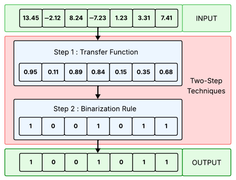 Figure 1
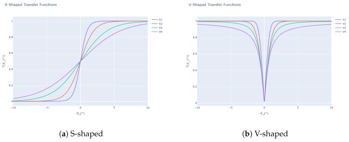 Figure 2
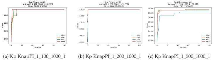 Figure 3
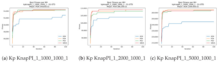 Figure 4
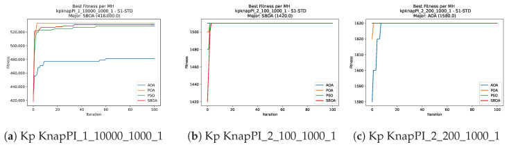 Figure 5
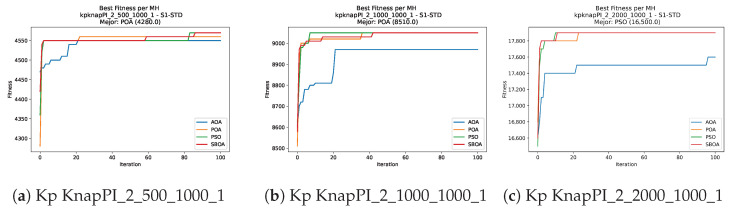 Figure 6
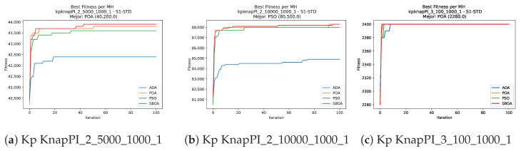 Figure 7
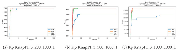 Figure 8
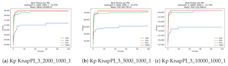 Figure 9
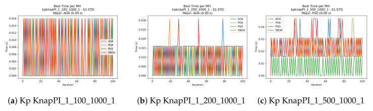 Figure 10
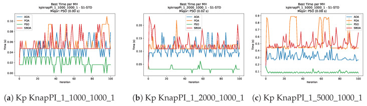 Figure 11
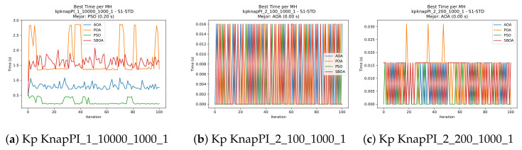 Figure 12
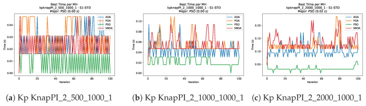 Figure 13
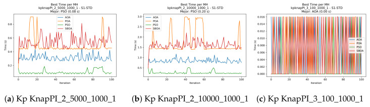 Figure 14
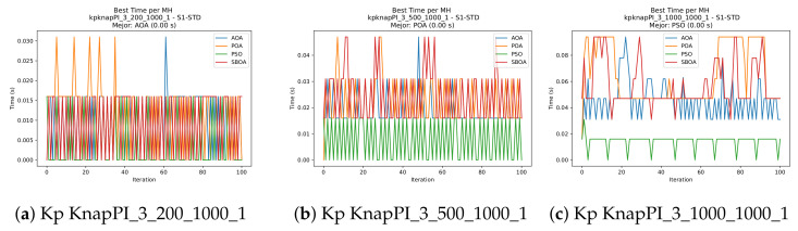 Figure 15
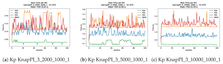 Figure 16
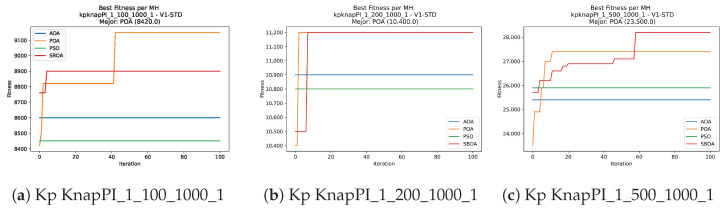 Figure 17
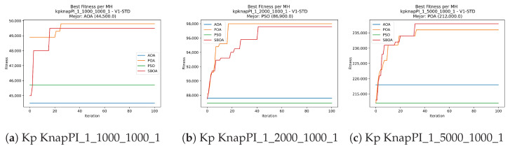 Figure 18
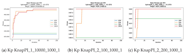 Figure 19
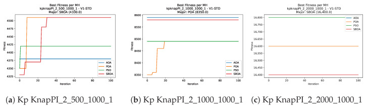 Figure 20
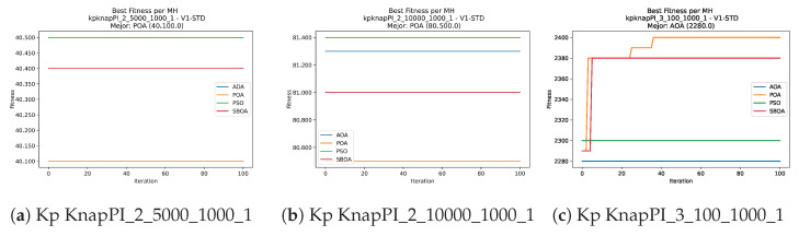 Figure 21
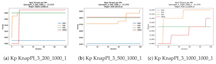 Figure 22
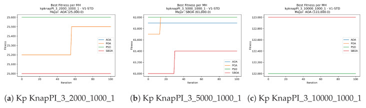 Figure 23
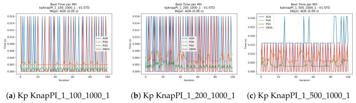 Figure 24
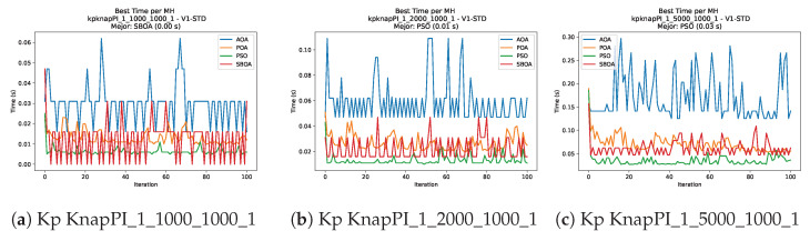 Figure 25
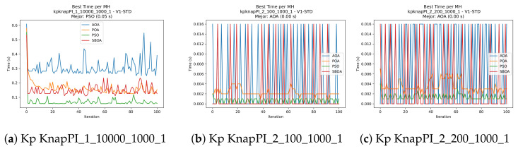 Figure 26
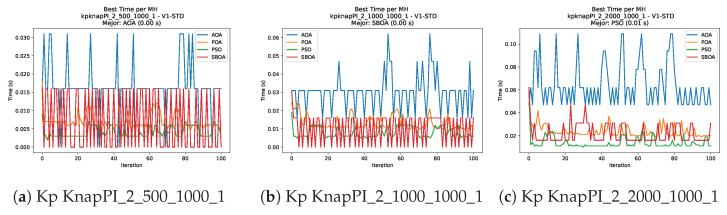 Figure 27
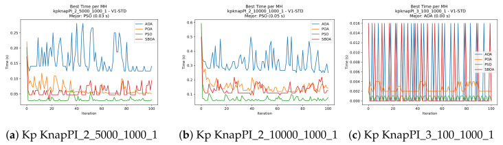 Figure 28
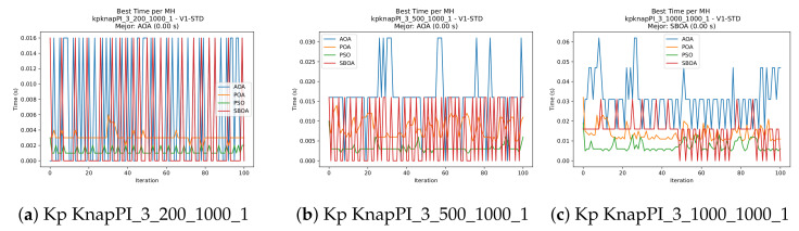 Figure 29
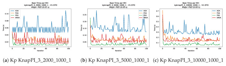 Figure 30
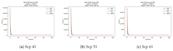 Figure 31
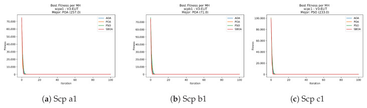 Figure 32
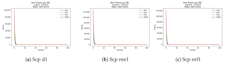 Figure 33
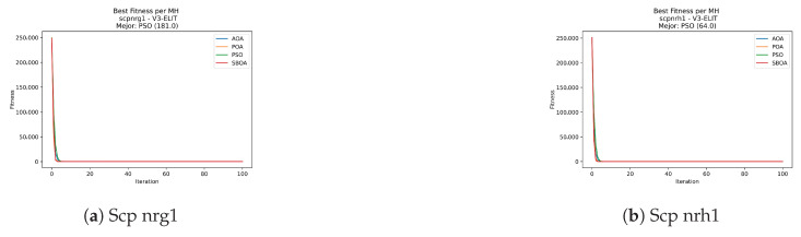 Figure 34
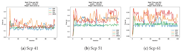 Figure 35
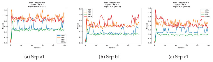 Figure 36
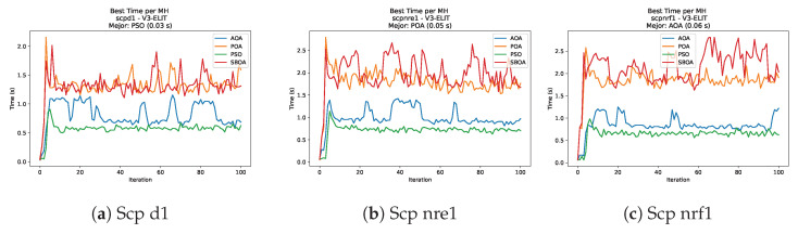 Figure 37
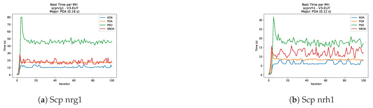 Figure 38
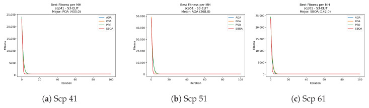 Figure 39
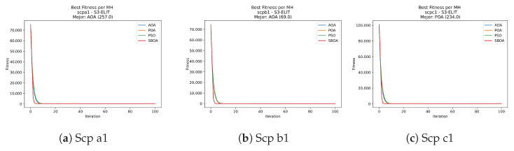 Figure 40
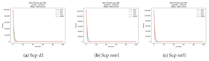 Figure 41
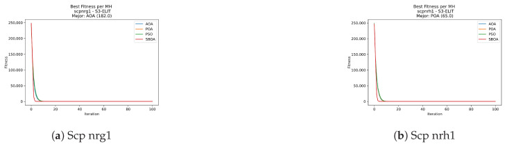 Figure 42
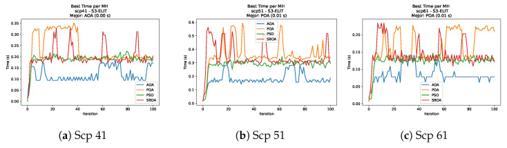 Figure 43
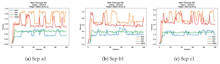 Figure 44
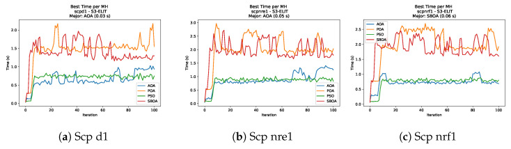 Figure 45
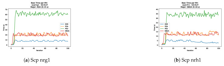 Figure 46
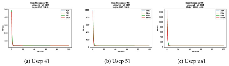 Figure 47
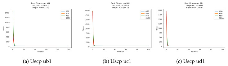 Figure 48
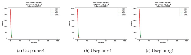 Figure 49
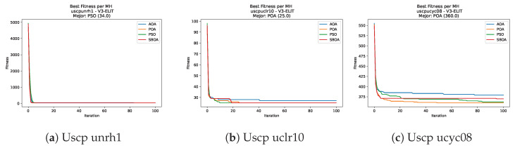 Figure 50
Peer Reviews
No public reviews on file for this paper yet. If you reviewed it on a platform where reviews are public (OpenReview, ICLR, NeurIPS, ICML), you can paste yours below so the community can read it here.
Videos
No videos yet. Explain this paper in a talk, walkthrough, or lecture? Add one.
Taxonomy
TopicsMetaheuristic Optimization Algorithms Research · Vehicle Routing Optimization Methods · Optimization and Packing Problems
1. Introduction
In today’s industry, there are significant combinatorial optimization problems such as the following: parameter optimization for cost prediction [1] (the optimization of reaction processes is crucial for the green, efficient, and sustainable development of the chemical industry [2]), optimization and robot path planning [3], and the optimization of parameters for monitoring in mining [4]. In these cases, metaheuristics are a tool for solving these problems, applying different algorithms as alternatives to exact methods. Methaheuristics are a real alternative when the problem is at a large scale, as their time is usually polynomial, achieving good solutions in a reasonable amount of time [5]. In general, metaheuristics can be applied to a wide variety of problems and have the flexibility to adapt to dynamic environments, making them suitable for different domains. These features make them highly appealing for solving real-world problems across multiple fields, including logistics [6,7], manufacturing [8,9], transportation [10,11], healthcare [12,13], and mining [14,15], among others.
However, there are another types of problems called binary problems, where the choice is to activate or deactivate a process, assign or not assign a task, or turn a machine on or off, among others. In general, these types of problems are NP-hard, which means that for large instances there are no efficient exact algorithms, meaning metaheuristics are a good-quality alternative solution with reasonable processing time. Binary metaheuristics have made contributions in a variety of industrial fields: in the logistics chain in general; in logistics in particular with regard to the allocation of routes and vehicles; in production planning when deciding which product to manufacture in different periods [16]; in the selection of financial asset portfolios under restrictions [17]; in the Crew Scheduling Problem in different areas such as maritime, land, and air where pilots, flight attendants, and drivers are assigned, taking into account a series of restrictions with the aim of minimizing costs and ensuring operations [18]; in the Workflow Scheduling in cloud computing data centers, with the aim of minimizing execution cost, execution time, and energy consumption [19]; in the security audit trail analysis problem where metaheuristics are used to improve the quality of intrusion detection [20]; in [21], a Z-shaped transfer function was used to solve the Knapsack Problem present in the industry; in [22], where a clustering-based binarization mechanism is explored to solve the Set Covering Problem, which allows modeling real-world problems where the goal is to minimize costs and maximize coverage; and in [23], where a robust Crow Search Algorithm (CSA) is proposed to solve both the optimal location of PMUs and the optimal static estimation for the entire electrical power system.
Exact algorithms (Branch and Bound or formulations based on mixed integer programming) can guarantee global optimality when the gap is zero, indicating that there is no better solution. However, these methods can have exponential behavior in the worst case for NP-complete problems, allowing metaheuristics to be an alternative solution at a lower computational cost, using exact solutions as a reference when they are available.
Within this landscape, the 0–1 Knapsack Problem (KP), the Set Covering Problem (SCP), and its unicost variant (USCP) are canonical NP-hard problems and are present in various industries [24]; notably, KP and SCP (and thus USCP) are among the 21 problems mentioned by Karp [25], and widely used as benchmarks due to their prevalence in real decision-making settings (KP) in resource selection under capacity constraints, and (SCP/USCP) in coverage- and facility-type decisions.
The use of metaheuristics to solve the KP and SCP includes algorithms such as Genetic Algorithms [26], Particle Swarm Optimization [27], the Secretary Bird Optimization Algorithm [28], the Whale Optimization Algorithm [29], the Grey Wolf Optimizer [30], the Arithmetic Optimization Algorithm [31], and the Fuzzy Hunter Optimizer [32], among others. In particular, binarization techniques have been explored to adapt metaheuristics designed for continuous optimization problems to the binary domain.
The presence of binary optimization problems in industry [33] and the use of metaheuristics leads us to take two practical approaches: on the one hand, it leads us to use algorithms created to work natively on these problems and, on the other hand, to use algorithms that were originally created to work in continuous spaces and to adapt them to work in binary spaces. Our work focuses on the second alternative, as we aim to offer a wider range of solutions for algorithms that were originally built for continuous spaces, allowing them to work in discrete environments. This is justified in order not to waste the maturity acquired by operators, such as the balance between exploration and exploitation, where POA achieves an effective balance [34,35].
The Pufferfish Optimization Algorithm (POA) is a recent bio-inspired metaheuristic that models exploration and exploitation via predator–prey dynamics and a defensive mechanism, showing competitive performance on continuous optimization tasks [36]. To apply POA (and, more generally, continuous metaheuristics) in binary combinatorial spaces such as KP and SCP, a binarization stage is required. A widely adopted approach is the two-step scheme: (i) a transfer function maps the continuous search outputs into , and (ii) a binarization rule discretizes them into [37,38]. Transfer functions are commonly grouped into two families with distinct behaviors: S-shaped (probabilistic switching) and V-shaped (bit-flip likelihood tied to movement magnitude) [37,38]. When coupled with standard discretization rules (e.g., probabilistic STD and elitist ELIT), these functions induce distinct exploration–exploitation trade-offs within the binary search space. To provide context and comparison, PSO, AOA, and SBOA serve as standard baselines due to their well-documented behavior and established binary adaptations [27].
This work investigates how the transfer function family (S-shaped vs. V-shaped) affects the performance of a binary POA (BPOA) across maximization and minimization problem classes. For KP (maximization), we compare S1-STD versus V1-STD; for SCP and USCP (minimization), we contrast S3-ELIT versus V3-ELIT.
Our study provides a controlled comparison that clarifies the algorithmic implications of S- vs. V-shaped dynamics in BPOA and offers practical guidance for selecting transfer–rule pairs according to problem type. Concretely, our contributions are as follows: a systematic S vs. V assessment of BPOA on KP and SCP/USCP using transfer–rule combinations grounded in the prior binarization literature [37,38], and an empirical analysis against a standard baseline (PSO, AOA, and SBOA) to contextualize the performance patterns [27].
This article is organized as follows. Section 2 presents the 0–1 Knapsack Problem and Set Covering Problem. Section 3 discusses how to resolve combinatorial problems with continuos metaheuristics. Section 4 reviews the Pufferfish Optimization Algorithm. Section 5 describes explains how and make the binary version of POA. Finally, we present our results, discussions, conclusions, and possible future lines of research in Section 6, Section 7 and Section 8.
2. Combinatorial Problems
In this section, we present the combinatorial problems used in our work: the 0–1 KnapSack Problem, Set Covering Problem, and Unicost Set Covering Problem. Solving these problems in the context of Industry 4.0 is very important, as they constitute a basic abstraction of problems present in the industry, such as: efficient resource allocation, the efficient planning of process activities, optimal supply chain management, the optimization of sensor placement and key actions in smart industry, and route planning to ensure customer coverage, among others. Consequently, these problems define a path to practical solutions in the new industrial revolution, the study and understanding of which facilitates real-time decision-making, a key element for competitiveness in today’s world.
The Industry 4.0, which is associated with the fourth industrial revolution, constantly challenges us to improve [39,40]. Its essence lies in automated and interconnected industrial production, where technology plays a central role. Its main objective is to create highly connected, flexible, and autonomous smart industries. Industry 4.0 aims to achieve maximum production efficiency alongside agile and flexible processes with a high capacity for adaptation, optimizing the use of resources at the lowest possible cost while maintaining quality [41]. Among its fundamental pillars are the following:
- The Internet of Things (IoT). This allows different devices such as machines, sensors, tools, and products to be connected for the purpose of obtaining real-time data [42].
- Big Data and Analytics. This allows you to store and analyze large volumes of collected data, enabling you to make preventive decisions. [43].
- Automation and Advanced Robotics. These facilitate or replace repetitive tasks performed by humans [44].
- Cloud computing. This enables cloud storage and processing, allowing fast and secure access [45].
- Cybersecurity. Given the current state of digital interconnection, it is necessary to protect data to avoid risks to the industry [46].
- Additive Manufacturing. This allows objects to be created digitally before being transferred to physical form, thereby preventing errors and losses [47].
- Augmented Reality. Allows you to simulate scenarios for staff training or product improvements under special conditions [48].
Optimization is fundamental in Industry 4.0, as the data generated allows for the improvement of different industrial processes, reducing waste and improving quality and efficiency [40,49,50]. In this sense, metaheuristics are a key tool for tackling real industrial problems, by finding efficient solutions in a timely manner [51,52].
2.1. 0–1 Knapsack Problem
The Knapsack Problem (KP) is a classic binary combinatorial optimization problem that falls into the category of NP-hard problems. Its primary objective is to select a subset of items that maximizes the total value without exceeding a predefined maximum capacity.
2.1.1. Formal
Mathematical Formulation
Formally, let be a set of n available items, where each item has an associated value and weight . Additionally, let W be the maximum weight capacity that the knapsack can hold. The problem consists of identifying an optimal subset of items that maximizes the total value without exceeding the maximum capacity W.
To model and computationally solve this problem, the formal set-based definition translates into a mathematical formulation using binary variables. We introduce the binary variable , which takes the value of one if the item is selected to be included in the knapsack, and the value of zero otherwise.
Thus, the primary objective is to maximize the total value of the selected items, summing only the values of the included items, as indicated by Equation (1).
The main constraint of the problem is the weight constraint, which ensures that the sum of the weights of the selected items does not exceed the maximum capacity W. This is represented by the following equation:
Additionally, it must be ensured that the decision variable is binary:
2.1.2. KP Practical Example
Suppose a process plant has a planned shutdown window of h to service a bottleneck machine. Each maintenance task requires a certain duration (hours) and yields an expected benefit (e.g., avoided downtime or cost savings). The decision is binary: execute the task ( ) or skip it ( ). The goal is to maximize the total benefit without exceeding W.
2.1.3. How the Optimal Set Is Obtained
To compute an optimal selection under the shutdown limit h, we can use the classical dynamic programming (DP) scheme for the 0–1 Knapsack. Let and denote the duration (hours) and the benefit of task i, respectively. Define
with base cases for all . The recurrence is
After filling the table up to , the selected tasks are recovered by backtracking; if , then task i is chosen ( ) and we set ; otherwise task i is skipped ( ). This yields an optimal set in time.
Multiple Optimal Solutions in This Instance
For the maintenance data in Table 1 (Section 2), the optimal value is . There are several optimal sets achieving this value, such as the following examples:
- Backup motor replacement (5 h, 80);
- Shaft alignment (3 h, 50);
- Advanced lubrication (2 h, 30);
- Backup motor replacement (5 h, 80);
- Belt replacement (4 h, 65);
- PLC update (1 h, 15);
- Shaft alignment (3 h, 50);
- Belt replacement (4 h, 65);
- Advanced lubrication (2 h, 30);
- PLC update (1 h, 15).
In the example shown previously we reported one of these optimal sets.
2.1.4. Sanity Check
To make the optimum “visible” at a glance, Table 2 lists the top feasible combinations (by value) not exceeding h. No feasible combination improves upon value 160.
Codes:
- SA = Shaft alignment;
- BR = Belt replacement;
- AL = Advanced lubrication;
- SC = Sensor calibration;
- PLC = PLC software update;
- BMR = Backup motor replacement.
This subsection clarifies both how the optimal solution is computed (DP with backtracking) and what it looks like (there can be multiple optimal sets with the same maximum value).
2.2. Set Covering Problem
The Set Covering Problem (SCP) is a classical NP-hard combinatorial optimization problem. Given a universe of requirements and a collection of candidate subsets (each with an associated cost), the goal is to select a minimum-cost family of subsets that collectively covers every requirement at least once.
2.2.1. Formal Mathematical Formulation
Let be the set of requirements and be a family of subsets , with cost . A binary matrix encodes coverage, where if and otherwise. Using binary decision variables to indicate whether subset is chosen, the SCP can be stated as follows:
2.2.2. SCP Practical Example
Consider a pipeline network divided into five critical inspection zones, . The maintenance team has predefined mobile inspection routes ; each route covers a subset of zones and has an execution time (cost). The objective is to choose the set of routes that covers all zones in the least total time as shown in Table 3.
Routes and Costs
We denote the cost in hours in parentheses:
2.2.3. Instance Formulation
Let if route is selected, and 0 otherwise. The model becomes
2.2.4. Optimal Solution
One optimal solution is to select routes with total cost h. These two routes jointly cover all zones:
No single route covers all zones, and any selection of two routes with total cost is infeasible (for completeness, another minimum-cost solution is with the same cost h).
2.3. Unicost Set Covering Problem
The unicost variant of the Set Covering Problem (SCP) assumes identical column costs (i.e., for all ). Consequently, the objective becomes selecting the fewest columns such that every row is covered at least once. This specialization emphasizes the structural aspect of coverage, abstracting away heterogeneous cost effects.
Mathematically, the model is as follows:
subject to
where indicates whether column j covers row i, is a binary decision variable (1 if column j is selected; 0 otherwise), I is the set of rows, and J is the set of columns.
As with the general SCP, the unicost case is NP-hard and is widely encountered in applications such as scheduling, logistics, and resource allocation.
3. Continuous Metaheuristics Solving Combinatorial Problems
To deploy the Pufferfish Optimization Algorithm (POA) across multiple binary combinatorial problems, specifically the 0–1 Knapsack Problem (KP), the Set Covering Problem (SCP), and its unicost variant (USCP) the original continuous domain search dynamics must be coupled to a unified binarization layer so that POA operates in while preserving each problem’s feasibility structure (capacity in KP; coverage in SCP/USCP). As discussed in Section 1, widely used continuous metaheuristics such as the Secretary Bird Optimization Algorithm [28], Arithmetic Optimization Algorithm [31], Grey Wolf Optimizer [30], and Particle Swarm Optimization [53] follow the same adaptation path: a two-step scheme in which (i) a transfer function (e.g., S-shaped or V-shaped) maps real-valued updates to {0,1}, and (ii) a binarization rule (e.g., standard, complement, or elitist) discretizes them into 0/1 decisions. In this work, we adopt that paradigm to endow POA with a common binary search interface and apply it, unchanged, across KP, SCP, and USCP, with only the objective and constraint handling being problem specific.
3.1. Two-Step Technique
In the literature, there are different ways to binarize continuous metaheuristics [38], but the most widely used is the two-step technique [37]. as its name implies, it carries out the binarization process in two phases. In the first phase, a transfer function is applied to convert continuous solutions into the real-valued domain [0,1]. Then, in the second phase, a binarization rule is used to discretize the transferred value, thereby completing the binarization process. Figure 1 provides a general overview of this technique.
3.2. Transfer and Binary Functions
In the literature [38], several transfer functions have been introduced to transform continuous outputs into binary decisions. These are typically divided into two principal categories according to their profile and operational behavior: the S-shaped family and the V-shaped family. Both groups are widely recognized as standard mechanisms for translating a continuous search domain into a discrete one.
S-Shaped Functions: Characterized by a sigmoidal curve, these functions output values in the interval , which can be interpreted as the likelihood of assigning a ‘1’ to a given component of the solution. Values near zero tend to yield probabilities close to 0.5, whereas large positive or negative inputs drive the probability towards 1 or 0, respectively. This behavior mimics a probabilistic switching process.V-Shaped Functions: Unlike the previous type, these functions link the probability of flipping a bit to the absolute magnitude of the continuous input, regardless of its sign. Small magnitudes lead to a low probability of change, while larger magnitudes increase that probability. This approach is conceptually related to the notion of movement intensity in swarm-based methods, where greater displacement is more likely to modify the current state of the solution.
Table 4 and Figure 2 summarize the representative transfer functions from both families that are frequently adopted in binary optimization studies. In these expressions, denotes the continuous value at the j-th dimension of the i-th candidate, obtained after applying the perturbation defined by the continuous metaheuristic.
Additionally, in the literature [38], we can find five different binarization rules, of which we highlight the following:
- Standard (STD): If the condition is satisfied, the standard binarization rule returns the value of 1; otherwise, it returns 0. Mathematically, it is defined as follows:
- Elitist (ELIT): The best value is assigned if a random value is within the probability; otherwise, a zero value is assigned. Mathematically, it is defined as follows:
4. Pufferfish Optimization Algorithm
The Pufferfish Optimization Algorithm (POA) is a bio-inspired metaheuristic proposed in 2024 by Al-Baik et al. [36], based on the natural defensive behavior of the pufferfish against its predators. This algorithm was originally designed to solve continuous optimization problems, using two main phases: exploration (predator attack) and exploitation (defense mechanism), aiming to efficiently find optimal solutions.
The algorithm operates in two primary phases that mimic the natural behavior of the pufferfish:
4.1. Exploration Phase
This phase models the predator attack on the pufferfish, driving a global exploration of the search space. The process is defined as follows:
- Candidate Prey Selection: Each member of the population acts as a predator. For each predator, the candidate prey (other pufferfish) are randomly selected among those individuals with better objective function values. The candidate prey set for predator i is defined as follows:
where
- – : The set of candidate prey for the i-th predator;
- – : The k-th population member, potential prey;
- – : The objective function value of the k-th population member;
- – : The objective function value of the i-th predator.
- Predator Movement Towards Prey: A new position for each predator is calculated in the solution space, simulating movement toward a randomly selected prey from the candidate set. This exploration strategy enables the discovery of promising regions in the search space. The movement is modeled by the following equation:
where
- – : New position of predator i in dimension j;
- – : Prey randomly selected from the set ;
- – : A random number uniformly distributed in ;
- – : A value randomly chosen as one or two, introducing variability in the movement.
In the implementation of the movement equations (Equations (11) and (12)), the random numbers are generated from a uniform distribution . The variability parameter I in Phase 1 is randomly selected from a discrete set .
4.2. Exploitation Phase
This phase captures the pufferfish’s defense mechanism against its predators, supporting a refined local search around promising regions:
- Predator Escape from Inflated Pufferfish: When attacked, the pufferfish inflates into a spiny ball, causing the predator to flee. This escape movement is translated into a local search strategy that helps to refine and exploit promising regions of the search space. The movement is modeled as follows:
where
- – : New position of predator i in dimension j;
- – , : Upper and lower bounds for dimension j;
- –t: Current iteration counter;
- – : A random number uniformly distributed in .
4.3. Solution Selection
A key aspect of POA is its greedy selection mechanism, similar to those used by other metaheuristics, which ensures continuous improvement or at least the preservation of solutions’ quality.
The quality of each solution is evaluated using the objective function F. After generating a candidate solution (in either the exploration or exploitation phase), the algorithm compares the fitness value of the new position with the current value .
The new solution is accepted only if it offers a better fitness value (i.e., a lower cost in a minimization problem). Otherwise, the current solution is retained. Formally, this is defined with the following update equation:
where represents a solution generated either by the predator movement or by the pufferfish’s defense mechanism. This update strategy ensures that the global quality of the population improves or at least remains stable in each iteration, thus guiding the search toward optimal solutions.
The pseudocode of POA is detailed in the pseudocode of Algorithm 1. Algorithm 1 Pseudocode of Pufferfish Optimization AlgorithmInput: Input problem information: variables, objective function, and constraints.Output: Best solution
- 1:Initialize the population randomly.
- 2:for do
- 3: for do
- 4: Exploration Phase:
- 5: Determine the candidate Pufferfish set for the i-th POA member Equation (10).
- 6: Select the target pufferfish for the ith POA member at random.
- 7: Calculate new position of ith POA member using Equation (11)
- 8: Update the i-th Pufferfish using Update Equation (13).
- 9: Exploitation Phase:
- 10: Calculate new position of ith POA member using Equation (12).
- 11: Update the i-th Pufferfish using Update Equation (13).
- 12: end for
- 13: Output the best quasi-optimal solution obtained with the POA.
- 14: Save the best candidate solution so far.
- 15:end for
- 16:Output the best quasi-optimal solution obtained with the POA.
5. Binary Pufferfish Optimization Algorithm
As explained in Section 4, the Pufferfish Optimization Algorithm (POA) is a metaheuristic originally designed to solve continuous optimization problems. To address combinatorial problems such as KP, SCP, and USCP, it is necessary to transform the solutions into the binary domain.
In this work, following Section 3, the two-step technique is employed, which is one of the most widely used approaches for binarizing continuous metaheuristics [37,38]. In this scheme, the first step corresponds to the application of transfer functions that map continuous values into the interval . For this purpose, S-shaped and V-shaped transfer functions are considered, as they provide a good balance between exploration and exploitation.
The second step corresponds to applying binarization rules that discretize the transferred values into zero or one. In this study, two well-known rules are considered: the standard rule (STD), which assigns a binary value based on a probabilistic threshold, and the elitist rule (ELIT), which favors the incorporation of the best solution found in the population.
By combining S-shaped and V-shaped transfer functions with the STD and ELIT binarization rules, we analyze the effect of these configurations on the performance of the algorithm. As reported in the literature [38], the choice of the transfer function and the binarization rule can significantly influence the quality of the solutions obtained.
With these configurations, the Binary Pufferfish Optimization Algorithm (BPOA) is constructed. The process begins with the initialization of binary solutions, which are updated in each iteration using Equations (10)–(13), which represent the specific movement equations of POA. After perturbation, the solutions temporarily leave the binary domain; therefore, the binarization process is applied using the selected combinations of S/V-shaped transfer functions and STD/ELIT rules. This cycle is repeated until the defined number of iterations is completed.
The pseudocode of BPOA is detailed in the pseudocode of Algorithm 2. Algorithm 2 Pseudocode of Binary Pufferfish Optimization AlgorithmInput: Input problem information: variables, objective function, and constraints.Output: Best solution
- 1:Initialize the population randomly.
- 2:for do
- 3: for do
- 4: Exploration Phase:
- 5: Determine the candidate Pufferfish set for the i-th POA member Equation (10).
- 6: Select the target pufferfish for the i-th POA member at random.
- 7: Calculate new position of i-th POA member using Equation (11)
- 8: Update the i-th Pufferfish using Update Equation (13).
- 9: Exploitation Phase:
- 10: Calculate new position of i-th POA member using Equation (12).
- 11: Update the i-th Pufferfish using Update Equation (13).
- 12: Binarization of population X
- 13: end for
- 14: Output the best quasi-optimal solution obtained with the POA.
- 15: Save the best candidate solution so far.
- 16:end for
- 17:Output the best quasi-optimal solution obtained with the POA.
5.1. Theoretical Justification of Binarization
A fundamental criticism of many binary adaptations is the lack of “algorithmic specificity”, as binarization often acts as a generic wrapper. We contend that our selection of the binarization scheme is intrinsically linked to POA’s core exploration and exploitation mechanics.
POA’s mechanics rely on two phases with distinct movement magnitudes:
- Phase 1 (Exploration): Equation (11) generates large-magnitude movements in the search space, designed to jump to new, promising regions.
- Phase 2 (Exploitation): Equation (12) generates decreasing-magnitude movements, as the term in the denominator shrinks the step size as iterations increase.
The suitability of the transfer function families (S-shaped vs. V-shaped) depends on their interaction with this mechanic:
- V-Shaped Functions (for SCP/USCP): These functions (e.g., V3) link the probability of flipping a bit (changing zero to one) to the magnitude of the movement. This couples perfectly with POA: in early iterations, the large movements from Phase 1 result in a high bit-flip probability, fostering exploration. In late iterations, the small movements from Phase 2 result in a low bit-flip probability, allowing the solution to stabilize (the “defense mechanism”).
- S-Shaped Functions (for KP): These functions (e.g., S1) interpret the continuous value as the probability of a bit being ’1’. This aligns conceptually with the nature of the KP, which is an “item selection” problem (deciding whether to include or not). POA’s movement generates a “desirability” vector, and the S-shaped function translates this into a selection probability.
5.2. Feasibility Handling
Once a continuous solution is binarized, it is likely to violate problem-specific constraints. Therefore, a problem-dependent heuristic repair mechanism is applied before its fitness is evaluated to ensure all solutions are feasible.
- For the Knapsack Problem (KP): The KP has a capacity constraint (2). For infeasible solutions (overweight), a greedy repair heuristic based on the profit-to-weight ratio ( ) is applied.
- Removal Phase: If the solution exceeds capacity, the algorithm iterates over included items in ascending order of their ratio (worst to best), removing them (setting to zero) until the solution becomes feasible.
- Addition Phase: Once feasible, the algorithm iterates over non-included items in descending order of their ratio (best to worst), adding them (setting to one) as long as the solution remains feasible. The final addition that causes infeasibility is reverted.
- For the Set Covering Problem (SCP/USCP): The SCP has coverage constraints (Equation (4)). For infeasible solutions (uncovered rows), a greedy trade-off heuristic is applied:
- –While the solution is infeasible, the algorithm identifies all uncovered rows. It then calculates a ratio (cost/number of newly covered rows) for every available column. The column with the most efficient (lowest) ratio is added to the solution (set to one). This process repeats until all rows are covered, ensuring feasibility.
5.3. Computational Complexity Analysis
To evaluate the computational overhead, we analyze the complexity per iteration. Let N be the population size, n the dimensionality (items/columns), m the number of constraints (rows, for SCP), and the cost of the repair function.
BPOA Complexity: The total complexity per iteration is . The term arises from the candidate prey search (Phase 1), and the term arises from applying binarization, repair, and evaluation to each individual.BPSO Complexity: The complexity is , as it lacks the prey search.
The repair cost is problem dependent:
- For KP: The repair is , dominated by the ratio sorting. The total BPOA complexity is .
- For SCP/USCP: The greedy repair iterates times (where is the number of columns needed to repair). Each step involves recalculating coverage and ratios, taking (or for sparse matrices). The repair complexity is . The total BPOA complexity is .
In all cases, the polynomial overhead explains the slightly higher computation times for BPOA observed in Section 7.
6. Experimental Results
To validate our proposal, we used benchmark instances from the OR-Library [55] covering the 0–1 Knapsack Problem (KP) [56], the Set Covering Problem (SCP) [57], and the Unicost Set Covering Problem (USCP) [58]. Our approach was compared against widely used metaheuristics: the Pufferfish Optimization Algorithm (POA) [36], Secretary Bird Optimization Algorithm (SBOA) [28], Arithmetic Optimization Algorithm (AOA) [31], and Particle Swarm Optimization (PSO) [27].
6.1. Experimental Methodology
Before performing the main experimentation, we conducted internal tests for parameter configuration across the three problem classes (KP, SCP, and USCP). Specifically, we explored the population size in the range with steps of ten, and probed iteration budgets .
Table 5 shows the subset of instances used for parameter configuration. We chose these instances because they are representative of small/medium/large cases in the OR-Library portfolio. The table lists the following: the instance name, the problem type, the instance size (KP: number of items; SCP/USCP: M rows, N columns, and density of ones), and the known optimum. This experiment was conducted in a team using a Windows 10 operating system, an Intel Core i9-10900 K 3.70 GHz Processor, and 64 GB of RAM. The algorithm implementation was developed in the Python (v3.11.9) programming language, utilizing libraries such as NumPy and SciPy. All experiments were executed in serial mode. To ensure statistical independence across the 31 executions, a fixed random seed was not used; instead, each run was initialized with a different seed to capture varied stochastic behavior.
Table 6 shows the pilot evidence supporting the choice of a population size of ten and an iteration budget of 100 for the subsequent experiments. For each selected instance, we report (over 31 runs) the best, worst, and average objective value together with the average runtime in seconds and minutes. These results indicate fast convergence and diminishing returns beyond 100 iterations, while keeping the runtime reasonable and comparable across methods/configurations.
To further substantiate the choice of transfer functions and binarization rules under this budget, Table 7 compares, for each selected instance, an S-shaped versus a V-shaped configuration with their customary discretization rules. We report the average objective value, the percentage gap to the known optimum, and the average runtime (31 runs; 100 iterations). In KP, S1-STD attains the smallest gaps (quality first) while V1-STD is markedly faster (speed first). In SCP/USCP, V3-ELIT systematically improves both cost and time against S3-ELIT, especially as the instance size grows.
6.2. Conclusion of the Pilot
With a population of ten, 100 iterations form a robust knee point across KP, SCP, and USCP, balancing solutions’ quality and the runtime. Under this budget, S1-STD (quality first) and V1-STD (speed first) are the recommended pairings for KP, while V3-ELIT clearly dominates S3-ELIT for SCP/USCP in both cost and time, justifying their use in the main experiments.
Table 8 shows the final experimental configuration. The global settings used by all metaheuristics (All MH), the method, and problem-specific parameters are highlighted.
6.3. KP, SCP, and USCP Instances Resolved
Table 9 presents the KP instances, indicating for each case the instance name (Instance), the number of items (Number of Items), and the known optimal value (Optimum).
Table 10 and Table 11 show the instances used for the SCP and USCP, respectively. Each record in these tables includes the instance name (Instance), the number of constraints (M), the number of decision variables (N), the density of ones in the matrix described in Section 2 (Density (%)), and the known optimal value (Optimum).
It should be noted that the optimal values highlighted in bold and underlined do not correspond to global optima, but rather to the best results reported in the literature.
6.4. Results of KP, SCP, and USCP
This subsection presents the results obtained by BPOA using the parameters established in Section 6.1. The performance of BPOA is compared against three other metaheuristics: Particle Swarm Optimization (PSO), Secretary Bird Optimization Algorithm (SBOA), and Arithmetic Optimization Algorithm (AOA). Table 12 and Table 13 present the detailed results for the Knapsack Problem (KP) using the S1-STD binarization scheme. For each algorithm and instance, we report the optimal value (Opt), the best value achieved (Best), the average fitness (Avg. fitness), the worst value (Worst), the standard deviation (Std. fitness), and the relative percentage deviation (RPD) over 31 independent executions [59].
The RPD allows us to know how close a solution is to the known optimum.
where is the objective function value returned by the algorithm under evaluation and is the best known or optimal value for the problem instance.
Convergence plots trace how the metaheuristic progressively discovers higher-quality solutions as the iteration count grows. Because practical applications demand good answers within a reasonable time, the goal is to reach strong solutions without an excessive number of iterations or computational overhead. Following Crawford et al. [60] and Lemus-Romani et al. [61], we document the search process with graphs that plot fitness against iteration. Figure 3, Figure 4, Figure 5, Figure 6, Figure 7, Figure 8 and Figure 9 present this relationship—with iterations on the x-axis and fitness on the y-axis—and they indicate the sound convergence behavior, with no evidence that the algorithm becomes trapped in a local optimum [62].
Table 14 and Table 15 summarizes runtime statistics for KP under S1–STD: minimum, maximum, average, and standard deviation (in seconds) over 31 runs for BPOA, SBOA, AOA, and PSO.
Figure 10, Figure 11, Figure 12, Figure 13, Figure 14, Figure 15 and Figure 16 show how the runtime analysis for the S1-STD configuration confirms that PSO consistently achieves the most efficient and stable execution times across all problem sizes. AOA follows as a competitive alternative, generally faster than SBOA and BPOA but with moderate variability. Conversely, BPOA and SBOA exhibit the highest computational overhead; specifically, BPOA displays noticeable spikes in large-scale instances, reflecting the intensive computational effort required to sustain its superior convergence accuracy.
Table 16 and Table 17 shows the KP solution quality when using the V1–STD binarization. The columns mirror those of Table 12 to enable a direct comparison of best/worst/mean performance and variability between BPOA, SBOA, AOA, and PSO.
Figure 17, Figure 18, Figure 19, Figure 20, Figure 21, Figure 22 and Figure 23 show that BPOA and SBOA exhibit robust step-wise convergence, consistently reaching superior fitness levels compared to the stagnant performance of AOA. While PSO occasionally achieves top results in specific instances, BPOA demonstrates the most reliable trajectory, securing high-quality solutions with minimal fluctuation across the dataset.
Table 18 and Table 19 lists the runtime statistics for KP with V1–STD, allowing a time efficiency comparison against S1–STD and between the metaheuristics.
Figure 24, Figure 25, Figure 26, Figure 27, Figure 28, Figure 29 and Figure 30 show the runtime distributions, demonstrating that PSO consistently maintains the lowest and most stable execution times. In contrast, AOA exhibits significant computational instability, characterized by frequent high-magnitude spikes that increase the overall cost. BPOA and SBOA occupy an intermediate position; notably, BPOA demonstrates a steady and predictable timing behavior, effectively balancing the overhead compared to the erratic fluctuations observed in AOA.
Table 20 reports the solution costs for the Set Covering Problem (SCP) using the V3–ELIT configuration. For each instance, we include the reference optimum, best/worst value, mean over 31 runs, and standard deviation.
Figure 31, Figure 32, Figure 33 and Figure 34 plot the convergence curves for SCP under V-shaped binarization, comparing POA, PSO, SBOA, and AOA. The results demonstrate that POA, PSO, and SBOA exhibit strong convergence behaviors and reach competitive final costs, whereas AOA tends to stabilize at higher values, yielding less effective solutions in most instances.
Table 21 presents the runtime statistics (min/max/avg/std, in seconds) for SCP under V3–ELIT, comparing the time performance of POA, PSO, SBOA, and AOA.
Figure 35, Figure 36, Figure 37 and Figure 38 report the runtime distributions for SCP with V-shaped binarization, comparing POA, PSO, SBOA, and AOA; the results indicate that PSO is generally the most time efficient, while SBOA and AOA exhibit significantly higher computational overheads, particularly in the larger instances.
Table 22 summarizes SCP solution quality with the S3–ELIT binarization, using the same metrics as in V3–ELIT to contrast S-shaped versus V-shaped behaviors.
Figure 39, Figure 40, Figure 41 and Figure 42 display convergence trajectories for SCP under S-shaped binarization, contrasting POA, PSO, SBOA, and AOA; the curves are nearly indistinguishable, with a similar early descent and virtually identical terminal costs.
Table 23 provides the SCP runtime summary with S3–ELIT, facilitating a time efficiency comparison against V3–ELIT and between the evaluated metaheuristics.
Figure 43, Figure 44, Figure 45 and Figure 46 illustrate the runtime behavior per iteration for SCP instances using the S3-ELIT binarization scheme. As observed in the plots, AOA consistently exhibits the lowest computational times, demonstrating superior efficiency. PSO follows as the second fastest algorithm, maintaining a stable performance. In contrast, POA and SBOA display significantly higher runtimes and greater variability across the iterations, indicating the higher computational cost of these methods in this specific configuration.
Table 24 compiles the solution quality for the Unicost Set Covering Problem (USCP) using V3-ELIT. We report the best values, the worst values, the mean, and dispersion over 31 runs, relative to the known optimum.
Figure 47, Figure 48, Figure 49 and Figure 50 show the convergence curves for USCP under V-shaped binarization across multiple instances and runs. As illustrated, POA and PSO exhibit the most rapid convergence rates, settling at nearly identical optimal costs. Notably, in complex instances such as ucyc08, both algorithms clearly outperform AOA and SBOA, demonstrating their superior scalability and search capability.
Table 25 shows the runtime statistics (min, max, average, and standard deviation, in seconds) for USCP with V3–ELIT, comparing BPOA, PSO, AOA, and SBOA.
Figure 51, Figure 52, Figure 53 and Figure 54 compare the runtime distributions for USCP with V-shaped binarization. PSO generally exhibits the lowest runtimes, demonstrating high speeds across most instances, although it shows instability in larger datasets (e.g., unrg1 and unrh1). Conversely, SBOA displays the highest computational overhead and variability. POA and AOA maintain stable, intermediate execution times, positioning themselves between the rapid performance of PSO and the higher costs of SBOA.
Table 26 presents USCP solution quality using S3-ELIT, with the same performance metrics as those used for V3-ELIT to highlight the impact of switching from V-shaped to S-shaped transfers.
Figure 55, Figure 56, Figure 57 and Figure 58 present the convergence profiles for USCP under S-shaped binarization; the trajectories overlap closely throughout, with matching early improvement and final costs that are effectively the same.
Table 27 reports the runtime statistics for USCP with S3–ELIT, enabling a direct time comparison with V3–ELIT and between BPOA, PSO, AOA, and SBOA.
Figure 59, Figure 60, Figure 61 and Figure 62 report the runtime outcomes for USCP with S-shaped binarization across instances and repetitions. AOA consistently achieves the lowest execution times, establishing itself as the most efficient method in this configuration. While PSO is competitive in smaller instances, it exhibits significant instability and high runtimes on larger datasets (e.g., unrg1 and unrh1), whereas POA maintains a stable, albeit higher, computational cost.
In the Knapsack Problem (KP), the S1-STD binarization scheme yields near-optimal and highly stable results across all algorithms, although POA and PSO maintain a slight consistency edge over AOA and SBOA; conversely, the V1-STD scheme drastically reduces the runtimes at the expense of solution quality, where AOA stands out for its speed but exhibits larger optimality gaps in large-scale instances. Regarding the Set Covering Problems (SCP and USCP), the V3-ELIT approach clearly outperforms S3-ELIT, delivering superior costs and execution times, whereas S3-ELIT demonstrates poor scalability, particularly with SBOA, which exhibits the highest computational overhead and variability. In terms of comparative performance, AOA consistently ranks as the fastest method, achieving the lowest execution times in most scenarios, although it is occasionally outperformed in terms of solution quality by POA and PSO in complex instances; PSO offers a strong balance, being rapid on smaller instances yet showing runtime instability on larger datasets, and POA demonstrates the highest stability and search capability in difficult scenarios, justifying its intermediate computational cost with high-quality solutions, while SBOA proves to be the least time efficient. Overall, the results suggest employing S1-STD for KP when quality is paramount and V1-STD for speed, and choosing V3-ELIT for SCP/USCP, selecting AOA for maximum speed or POA/PSO for an optimal trade-off between solution quality and stability.
6.5. Statistical Test
To statistically validate our work, we considered the POA and PSO executions for the KP, SCP, and USCP problems. Our statistical analysis is based on two stages, according to [57]. The first stage consists of determining whether the data behaves normally, for which we use the Shapiro–Wilk test [63], as shown in Table 28, Table 29, Table 30, Table 31 and Table 32, where W represents the Shapiro–Wilk statistic, whose value is between [0,1], and the p-value is the probability of obtaining the observed data. As can be seen, the data does not follow a normal trend. To apply the test, we use the scipy.stats function in Python.
In the second stage of our analysis, given that our data does not follow a normal distribution, we used a nonparametric test, which in this case is the Mann–Whitney test. This test is used when two samples are independent and the validity of one of them cannot be assumed. We considered the following hypotheses: H_0_: Algorithm A ≥ Algorithm B, H_1_: Algorithm A < Algorithm B, where Algorithm A and Algorithm B represent the average value delivered by algorithms A and B. In two independent and uncorrelated data sets, we use the p-value to determine whether they are significantly different. In this sense, we consider that if the p-value is less than 0.05, the null hypothesis will be rejected, and the alternative hypothesis will be accepted. To apply the test, we use the scipy.stats function in Python. The application of the Mann–Whitney test is shown in Table 33, Table 34 and Table 35.
The Mann–Whitney test applied to the different problems with the selected pairs of techniques did not reveal statistically significant differences between the metaheuristics, as most of the p-values were greater than 0.05. Therefore, the null hypothesis could not be rejected.
7. Discussion
The empirical results validate our theoretical hypothesis (Section 5.1) regarding the synergy between POA’s mechanics and the chosen binarization scheme. For SCP/USCP, the superiority of V3–ELIT is not coincidental: POA’s Phase 1 (Exploration) generates high-magnitude movements, which the V-shaped function translates into a high bit-flip probability, fostering diversity. Conversely, Phase 2 (Exploitation) generates decreasing-magnitude movements, which the V-shaped function translates into solution stabilization, enabling convergence. S3–ELIT, lacking this coupling to movement magnitude, fails to achieve this dynamic translation.
This study investigated a binary instantiation of the Pufferfish Optimization Algorithm (BPOA) on three canonical 0–1 problems, KP, SCP, and USCP, via the two-step technique using representative S-shaped and V-shaped transfer functions combined with STD and ELIT binarization rules, benchmarking against PSO under a common budget (Table 8). The empirical evidence in Table 12, Table 13, Table 14, Table 15, Table 16, Table 17, Table 18, Table 19, Table 20, Table 21, Table 22, Table 23, Table 24, Table 25, Table 26 and Table 27 reveals several robust patterns that we summarize below.
For KP, S1–STD delivers near-optimal, low-variance solutions over a wide range of sizes, while V1–STD yields markedly shorter runtimes at the expense of larger optimality gaps and variability (cf. Table 12 and Table 14 vs. Table 16 and Table 18). This establishes a clear quality–speed trade-off: S1–STD is the quality-first option; V1–STD is a pragmatic choice when tight wall-time constraints prevail.
For coverage minimization (SCP/USCP), V3–ELIT consistently outperforms S3–ELIT in terms of solutions’ cost, robustness, and scalability, with especially clear advantages in large/dense instances, where S3–ELIT’s runtime escalates sharply (cf. Table 20, Table 21, Table 22, Table 23, Table 24, Table 25, Table 26 and Table 27). Thus, for coverage problems, the V-shaped transfer with an elitist rule provides the most favorable quality–efficiency balance.
Once an effective transfer–rule pairing is fixed, the search engine plays a secondary role: PSO is generally faster, while BPOA is occasionally more stable or slightly tighter in terms of the best/mean cost in the hardest instances, framing a time–stability trade-off. Complementarily, Wilcoxon–Mann–Whitney tests over 31 runs mostly return when the methods are already near optimum (e.g., KP with S1–STD; several SCP/USCP cases under V3–ELIT) and show significance precisely where descriptive gaps are large, reinforcing that discretization design is the principal performance driver and the choice between BPOA and PSO mainly modulates runtime and stability.
Mechanistically, these results align with bit-flip dynamics: S-shaped transfers with STD behave as probability thresholds that stabilize packing decisions in KP’s profit–weight landscape (hence S1–STD’s low variance), whereas V-shaped transfers increase flip probability with movement magnitude, promoting faster but less predictable exploration (V1–STD). For coverage problems, ELIT’s guidance from the incumbent best is crucial in order to propagate structural improvements under constraints, and V3’s smooth, saturating map supplies moderated but persistent flips, explaining V3–ELIT’s superior quality–efficiency trade-off. The limitations of this study include its reliance on OR-Library benchmarks and fixed budgets (Table 8), exploration of a restricted subset of transfers/rules (S1/S3 and V1/V3; STD/ELIT), standard repair/feasibility checks that could interact with pairings, and and per-instance Wilcoxon tests without multiple comparison control or effect sizes; nevertheless, across the problems and sizes, the picture remains internally consistent and practically actionable, yielding clear guidance regarding when to favor quality-first vs. speed-first settings.
8. Conclusions
Within the context of the importance of optimization for Industry 4.0, we presented a unified binary adaptation of POA and evaluated its effectiveness on KP, SCP, and USCP under representative transfer-–rule designs, contrasting it with PSO, AOA, and SBOA under identical computational budgets. Three main conclusions follow from the experimental evidence.
For KP, S1–STD is the most reliable configuration, delivering near-optimal, low-variance solutions across sizes while V1–STD offers a compelling speed-first regime with a predictable trade-off in optimality gap and variability. Practitioners should select between these regimes based on the wall-time constraints and acceptable deviation from the optimum.
For SCP/USCP, the discretization pairing dominates performance: V3–ELIT consistently surpasses S3–ELIT in cost, robustness, and scalability, especially in large/dense instances. This indicates that moderated flip dynamics guided by elitism are better suited to coverage minimization than S-shaped thresholds.
Between BPOA and the other algorithms, once a good combination has been chosen, the solvers achieve comparable quality. AOA is usually faster, while BPOA can be slightly more accurate or stable in difficult cases with higher computational cost; therefore, the choice of method mainly adjusts the speed–stability profile rather than determining absolute performance. Therefore, the practical recommendations are as follows: use S1–STD for KP when quality is paramount and V1–STD with strict time budgets; prefer V3–ELIT for SCP/USCP to obtain better costs with manageable execution times; select the other algorithms for performance-oriented scenarios; and select BPOA when incremental gains or stability justify additional computation. Future work will expand the design space (additional S/V transfers and rules), develop adaptive/hybrid schedules that alternate transfer and rule during execution, integrate problem-aware repairs and lightweight local improvements for coverage, adopt dynamic population/budget allocation, strengthen inference with multiple comparison procedures and effect sizes, and validate on larger and more heterogeneous industrial instances to assess generalization and cost–quality scalability.
The reference list from the paper itself. Each links out to its DOI / PubMed record.
- 1Elmasry N.H. Elshaarawy M.K. Hybrid metaheuristic optimized Catboost models for construction cost estimation of concrete solid slabs Sci. Rep.2025152161210.1038/s 41598-025-06380-440596461 PMC 12215946 · doi ↗ · pubmed ↗
- 2Zhang D. Ouyang B. Luo Z.H. Reaction process optimization based on interpretable machine learning and metaheuristic optimization algorithms Chin. J. Chem. Eng.202584778510.1016/j.cjche.2025.02.001 · doi ↗
- 3García E. Villar J.R. Sedano J. Chira C. de la Cal E. Sánchez L. Slime Mould Metaheuristic for optimization and robot path planning Neurocomputing 202564713055110.1016/j.neucom.2025.130551 · doi ↗
- 4Laayati O. El Hadraoui H. El Maghraoui A. Guennouni N. Mekhfioui M. Chebak A. Metaheuristic-Optimized Forecasting in a Smart Edge—Fog—Cloud Energy Management Framework: An Industrial Mining Case Study Results Eng.20252810730310.1016/j.rineng.2025.107303 · doi ↗
- 5Mechaacha A. Belkaid F. Brahimi N. Multi-objective multi-product process planning with reconfigurable machines: Exact and metaheuristic approaches Expert Syst. Appl.202529812959110.1016/j.eswa.2025.129591 · doi ↗
- 6Ghotb S. Sowlati T. Mortyn J. Scheduling of log logistics using a metaheuristic approach Expert Syst. Appl.202423812200810.1016/j.eswa.2023.122008 · doi ↗
- 7Núñez-López J.M. Segovia-Hernández J.G. Sánchez-Ramírez E. Ponce-Ortega J.M. Integrating metaheuristic methods and deterministic strategies for optimizing supply chain equipment design in process engineering Chem. Eng. Res. Des.20252149310410.1016/j.cherd.2024.12.021 · doi ↗
- 8Dhouib S. Zouari A. Adaptive iterated stochastic metaheuristic to optimize holes drilling path in manufacturing industry: The Adaptive-Dhouib-Matrix-3 (A-DM 3)Eng. Appl. Artif. Intell.202312010589810.1016/j.engappai.2023.105898 · doi ↗