Multi-Strategy Fusion Improved Walrus Optimization Algorithm for Coverage Optimization in Wireless Sensor Networks
Ling Li, Youyi Ding, Xiancun Zhou, Xuemei Zhu, Zongling Wu, Wei Peng, Jingya Zhang, Chaochuan Jia

TL;DR
This paper improves the Walrus Optimization algorithm to better solve complex optimization problems in wireless sensor networks.
Contribution
A novel improved Walrus Optimization algorithm combining DE/best/1, LSC Mapping, and Beta-OBL strategies for enhanced performance.
Findings
IMWO achieved first place in average fitness rankings on CEC2017 and CEC2022 benchmark tests.
IMWO achieved 95.86% and 96.48% average coverage rates in WSN experiments, outperforming other algorithms.
Abstract
The Walrus Optimization (WO) algorithm, a metaheuristic inspired by walrus behavior, is known for its competitive convergence speed and effectiveness in solving high-dimensional and practical engineering optimization problems. However, it suffers from a tendency to converge to local optima and exhibits instability during the iterative process. To overcome these limitations, this study proposes an improved WO (IMWO) algorithm based on the integration of Differential Evolution/best/1 (DE/best/1) mutation, Logistics–Sine–Cosine (LSC) Mapping, and the Beta Opposition-Based Learning (Beta-OBL) strategy. These strategies work synergistically to enhance the algorithm’s global exploration capability, improve its search stability, and accelerate convergence with higher precision. The performance of the IMWO algorithm was comprehensively evaluated using the CEC2017 and CEC2022 benchmark test…
Click any figure to enlarge with its caption.
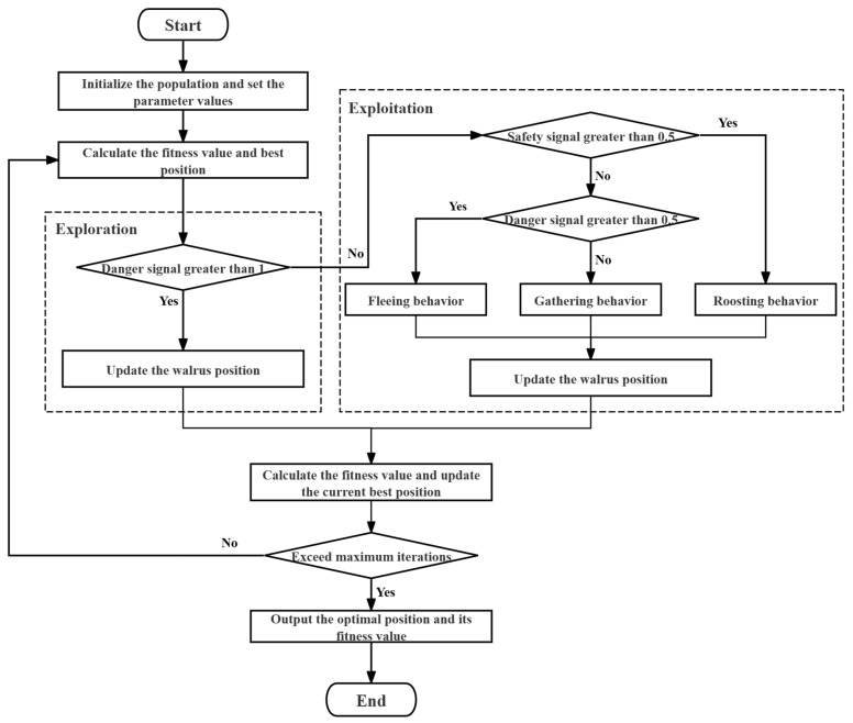 Figure 1
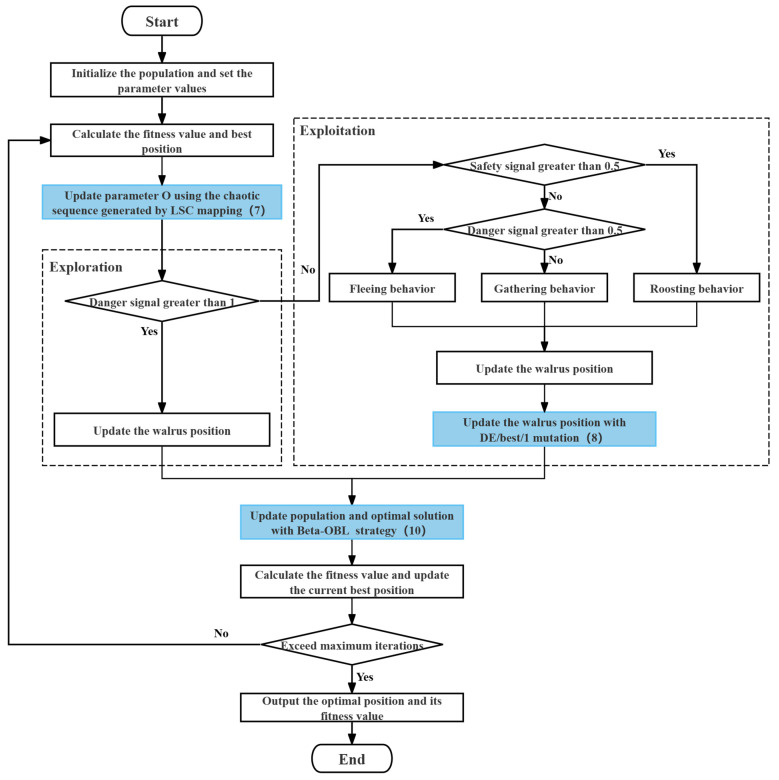 Figure 2
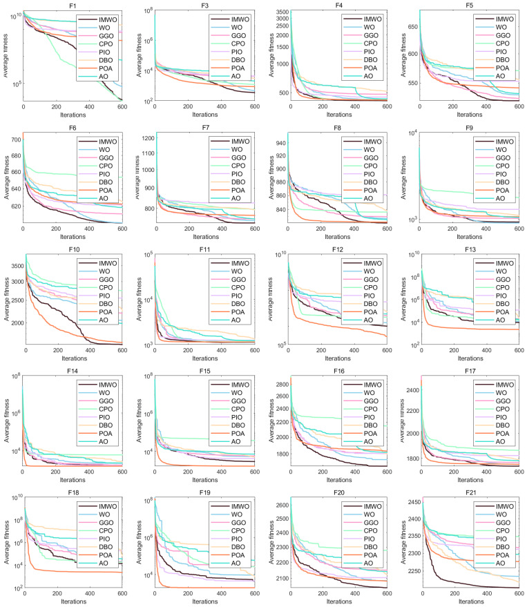 Figure 3
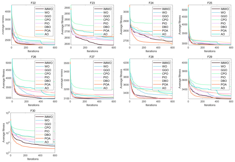 Figure 4
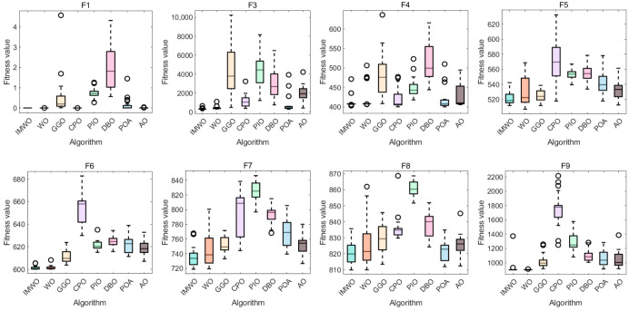 Figure 5
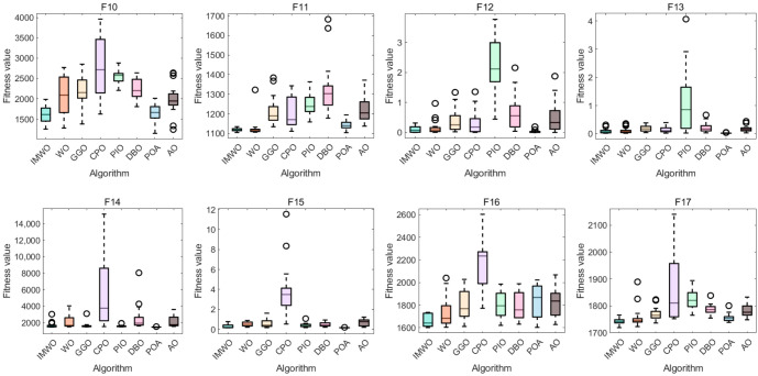 Figure 6
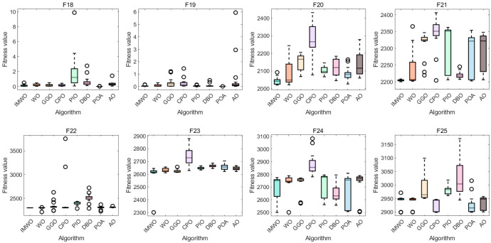 Figure 7
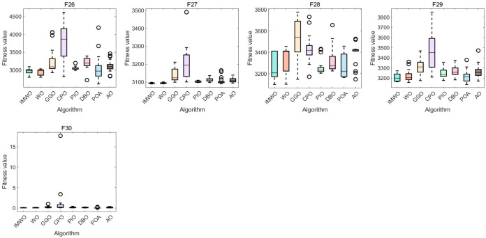 Figure 8
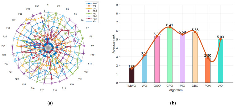 Figure 9
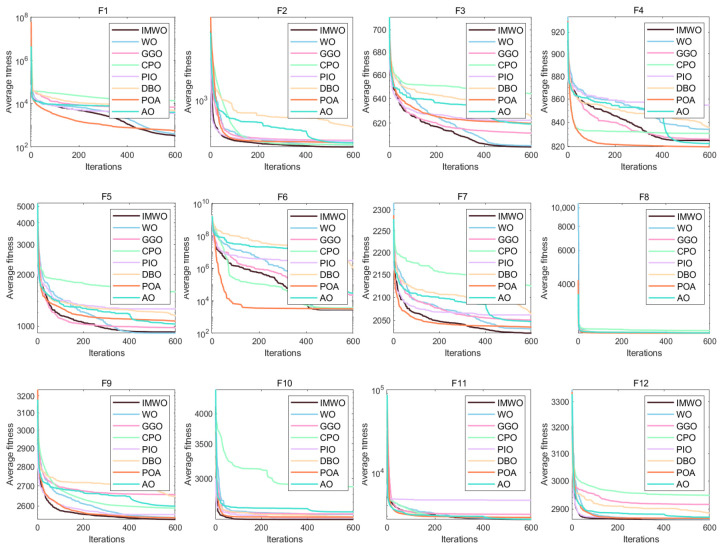 Figure 10
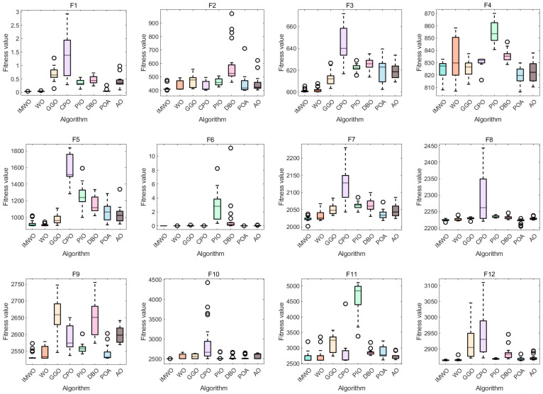 Figure 11
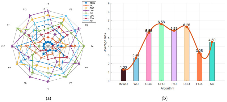 Figure 12
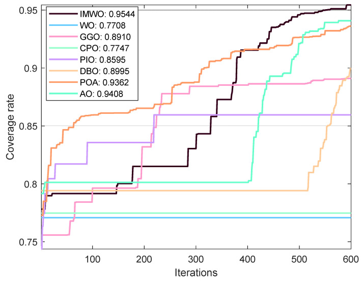 Figure 13
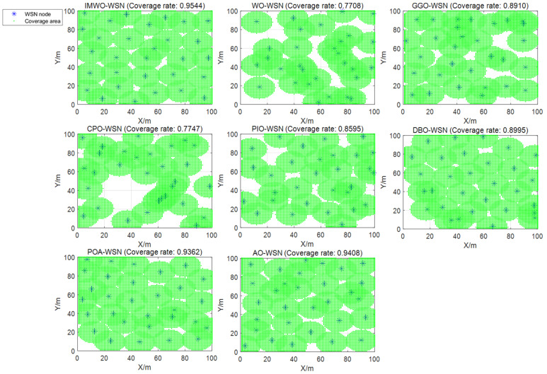 Figure 14
 Figure 15
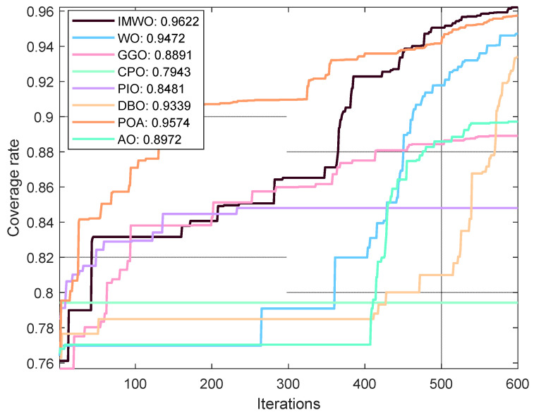 Figure 16
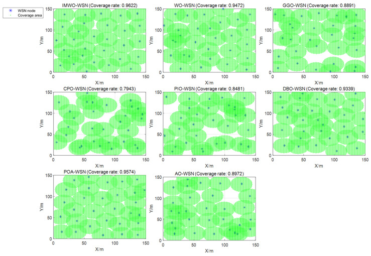 Figure 17
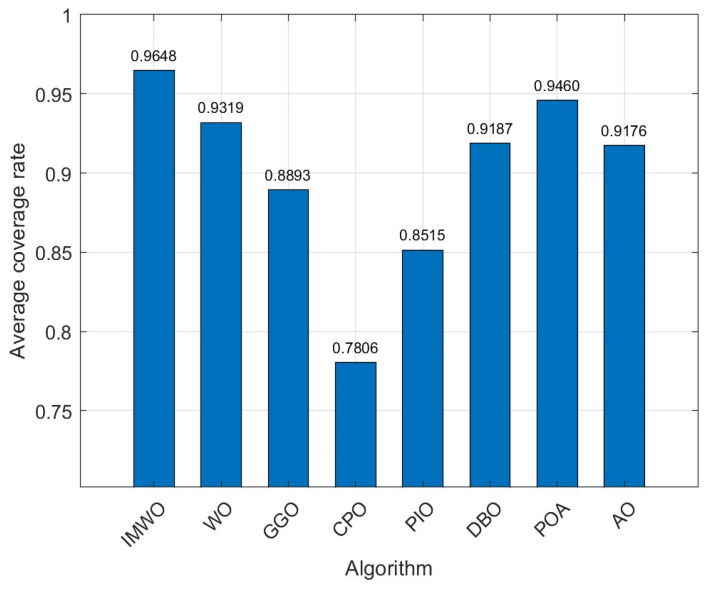 Figure 18
- —Major Projects for Natural Science Research in Anhui Universities
- —Startup Funding Project for High-Level Talents at West Anhui University
- —Open Research Projects of Anhui Dabie Mountain Traditional Chinese Medicine Research Institute
- —Key Projects of Natural Science Research in Anhui Universities
Peer Reviews
No public reviews on file for this paper yet. If you reviewed it on a platform where reviews are public (OpenReview, ICLR, NeurIPS, ICML), you can paste yours below so the community can read it here.
Videos
No videos yet. Explain this paper in a talk, walkthrough, or lecture? Add one.
Taxonomy
TopicsEnergy Efficient Wireless Sensor Networks · Metaheuristic Optimization Algorithms Research · Advanced Technologies in Various Fields
1. Introduction
Against the backdrop of the rapidly evolving Internet of Things (IoT) technology, WSNs, as the core carrier of information perception and transmission, have been deeply integrated into many key areas, such as smart agriculture and smart cities [1,2,3]. The coverage quality of WSNs directly impacts the comprehensiveness of data collection and the credibility of decision making. Their core optimization goal is to maximize the coverage of monitoring areas under limited node resources and energy constraints, while reducing perceived blind spots. However, traditional random deployment or static layout strategies often encounter problems such as uneven coverage and rapid energy consumption when facing large-scale networks or complex terrain, making it difficult to fully meet the application requirements of practical scenarios [4]. Therefore, optimizing the deployment strategy of sensor nodes through the application of intelligent optimization algorithms has become a core research topic for enhancing the performance of WSNs.
Metaheuristic algorithms, with their powerful global optimization capabilities, have been widely applied in the field of WSN coverage optimization [5]. Swarm intelligence optimization algorithms represent an important branch of metaheuristic algorithms inspired by the collaborative behaviors of swarm organisms in nature (such as ant colonies, bee colonies, and bird flocks) [6]. Their core characteristic is the achievement of global optimization through local interactions among multiple individuals, with information sharing and collaboration among individuals being key. As research deepens, new algorithms continue to emerge. In classic algorithms, Kennedy and Eberhart proposed the particle swarm optimization (PSO) algorithm [7] inspired by the foraging behavior of birds, but it tends to fall into local optima due to the decline in population diversity in the later stage. The cuckoo search (CS) algorithm proposed by Yang relies on Lévy flight to update the position [8], but the convergence accuracy is significantly affected by the flight step size. The gray wolf optimizer (GWO) [9] algorithm and whale optimization algorithm (WOA) [10] proposed by Mirjalili et al. imitate gray wolf hunting and humpback whale bubble net hunting, respectively, but they have the problem of low search efficiency in the later stage. Dorigo et al.’s ant colony optimization (ACO) algorithm [11] and Karaboga’s artificial bee colony (ABC) algorithm [12] perform well in combinatorial optimization, but exhibit insufficient adaptability when applied to WSN coverage optimization in continuous space. In emerging algorithms, Xiao et al.’s artificial lemming algorithm (ALA) [13], Almutairi and Shaheen’s kangaroo escape optimization technique (KET) [14], Martínez Gámez et al.’s tetragonula carbonaria optimization algorithm (TGCOA) [15], Sánchez Cortez et al.’s mantis shrimp optimization algorithm (MShOA) [16], etc., although imitating unique natural behaviors, focus on improving a single search mechanism and fail to effectively balance the dynamic relationship between exploration and exploitation. Xiao et al. proposed the multi-strategy boosted snow ablation optimizer (MSAO) [17] and the joint opposite selection-based arithmetic artificial rabbits optimization algorithm (MAROAOA) [18], which imitate unique natural behaviors and integrate multiple strategies. However, they still have limitations: MSAO tends to suffer from insufficient local exploitation precision in the late iteration stage, while MAROAOA incurs excessive computational overhead due to its complex opposite selection mechanism, resulting in difficulty in effectively balancing the dynamic trade-off between exploration and exploitation. Among them, the WO algorithm [19] proposed by Han et al. searches for the optimal solution through two stages of migration (exploration) and reproduction (exploitation). The structure is simple and easy to implement, but it has significant flaws: First, population update relies on the historical optimal information of individuals, which can easily lead to a lack of population diversity in the later stages of iteration, and it is difficult to jump out of the local optimum in multi-peak coverage scenarios. Second, the risk factors adopt a linear decreasing mode with a fixed variation pattern, resulting in insufficient exploration in the early stage and a tendency to stagnate in the later stage.
In recent years, many swarm intelligence optimization algorithms have been applied to research on coverage optimization in WSNs. For example, Liao et al. used the glowworm swarm optimization (GSO) algorithm [20] to expand the post-deployment coverage area, but failed to address the premature convergence problem. Saravanan et al. introduced the WO algorithm into WSN node coverage enhancement technology [21], but did not mitigate the inherent defects of the WO algorithm itself. Das et al. proposed the termite colony optimization (TCO) algorithm [22] to balance coverage and the number of sensors. Deif et al. combined the local search ACO algorithm [23] to optimize deployment cost and reliability. Mohar et al. improved coverage based on the bat algorithm (BA) [24]. However, these studies were mostly based on the direct application of basic algorithms and lacked ideas for systematic improvement. To overcome the bottleneck of traditional algorithms, scholars have proposed a variety of multi-strategy improvement schemes, but there are still obvious shortcomings: Chen et al. proposed a multi-strategy improved sparrow search algorithm (IM-DTSSA) [25] for WSN coverage optimization, but the strategy fusion lacks synergy and the global exploration breadth is insufficient. Li et al. proposed the virtual force-guided improved sand cat swarm optimization (VF-ISCSO) [26]; although it can reduce coverage blind spots, it relies too heavily on the virtual force mechanism and has limited local development accuracy. Chang et al. proposed a variant of the tuna swarm optimization algorithm based on the behavior evaluation and simplex strategy (SITSO) [27]; it has slow convergence and poor adaptability to multimodal scenarios. Wang et al. introduced a novel self-adaptive multi-strategy artificial bee colony (SaMABC) [28] that enhances optimization performance but has insufficient population diversity maintenance capabilities and is prone to late convergence stagnation. Liang et al. designed a new adaptive Cauchy variant butterfly optimization algorithm (ACBOA) [29], which can improve network coverage, but the dynamic balance control of exploration and development is insufficient. Deepa et al. proposed the Lévy Flight mechanism and the whale optimization algorithm (LWOA) [30], which enhance global exploration capabilities but ignore the collaborative improvement of local fine search and convergence stability.
In view of the shortcomings of the WO algorithm and those of existing improved algorithms, this study proposes an IMWO algorithm that integrates multiple enhancement strategies and applies it to WSN coverage optimization. The core improvements include three collaborative strategies: LSC Mapping [31] is adopted to increase the randomness through the ergodicity and pseudo-randomness of chaotic sequences, which introduces disturbance to expand population diversity. This helps maintain the global search intensity in the early stages while preserving local development disturbance in later stages, thereby balancing exploration and exploitation and improving the algorithm’s convergence accuracy and stability. The DE/best/1 mutation strategy [32] is introduced, drawing on the mutation mechanism based on the optimal individual in the differential evolution algorithm to enhance the algorithm’s ability to escape local optima and improve global search performance. It integrates Beta-OBL [33], which generates opposite solutions of current solutions to provide high-quality candidate individuals, thereby accelerating the convergence speed and improving coverage optimization efficiency.
Compared with existing multi-strategy algorithms, the distinctiveness of IMWO lies not in the simple superposition of strategies, but in the collaborative interaction of its three mechanisms to address core algorithmic deficiencies. Specifically, the DE/best/1 mutation compensates for the insufficient global exploration in algorithms such as IM-DTSSA and SaMABC. The LSC Mapping overcomes the weak maintenance of population diversity in algorithms such as SaMABC. The Beta-OBL strategy mitigates the slow convergence and poor stability observed in algorithms such as ISCSO and LWOA, ultimately achieving a dynamic balance between exploration and development capabilities. Research has found that not only does the IMWO algorithm show better overall performance in function optimization, but its joint improvement strategy can also effectively improve global search capabilities and convergence efficiency. In WSN coverage optimization, the coverage rate achieved by IMWO is significantly higher than that of the comparison algorithms, validating its superiority in solving practical problems. This study provides an efficient solution for improving the perceived performance of WSNs by improving the WO algorithm and applying it to WSN coverage optimization.
The main contributions of this study are summarized as follows:
- (1)The proposal of an IMWO algorithm by integrating DE/best/1 mutation, LSC Mapping, and Beta-OBL strategies, which effectively solves the defects of the original WO algorithm, such as easily falling into local optima and insufficient stability.
- (2)Establishing a complete mathematical model for WSN coverage optimization, including an objective function, constraint equations, and an encoding scheme, provides a theoretical basis for the application of intelligent optimization algorithms in this field.
- (3)Conducting comprehensive experiments on CEC2017/2022 benchmark suites and WSN coverage scenarios, verifying the superiority of IMWO in terms of scalability, robustness, and practical application value.
The remainder of this paper is organized as follows: Section 2 introduces the basic principles of WO. Section 3 presents the basic principles of IMWO. Section 4 validates the effectiveness of IMWO using the CEC2017 and CEC2022 standard function test suites. Section 5 introduces the wireless sensor network coverage model and provides experimental analysis and discussion on the application of IMWO to the WSN coverage problem. Section 6 concludes the paper and outlines future work.
2. Walrus Optimization Algorithm, WO
In 2024, M. Han et al. [19], inspired by the natural behaviors of walrus populations, proposed the WO algorithm. Specifically, upon receiving key signals such as danger and safety signals, walruses make behavioral choices such as migration, reproduction, habitat selection, foraging, aggregation, and escape. The WO algorithm draws ideas from these behaviors. In the mathematical model of this algorithm, the search space refers to the range within which the algorithm explores for optimal solutions, typically represented as a multi-dimensional space defined by the decision variables of the problem. The solution space encompasses all potential solutions, with each solution analogous to the position of a walrus in the search space, representing a potential solution to the problem. It can be a vector, where each component corresponds to the value of a decision variable, although the decision variables are determined by the specific problem. The core task of the WO algorithm is to find the optimal solution in the search space that minimizes or maximizes the objective function of the optimization problem.
2.1. Danger Signal and Safety Signal
The walrus swarm dynamically adjusts its behavior through an alert mechanism. The danger signal (DS) in WO is defined as shown in formula (1).
The safety signal (SS) is defined as shown in formula (4).
Here, O and K are danger factors, t denotes the current iteration number, and T denotes the maximum number of iterations allowed in the process. Additionally, both parameters and are randomly generated values, confined to the interval (0,1).
2.2. Migration (Exploration)
When the danger signal value exceeds 1, the walrus herd will migrate to areas more conducive to the survival of their population. During this migration phase of the walrus herd, the update method for their position is shown in formula (5), which specifies the specific rules for adjusting the position of the walrus at this stage.
Among them, and denote the new position and current position of the i-th walrus in the j-th dimension, respectively.
MS represents the movement step length of walruses, which determines the magnitude of positional change. In specific calculations, it is obtained by multiplying the positional difference between two randomly selected guardian walruses by the control factor and the square of a random number within the interval (0,1).
2.3. Reproduction (Exploitation)
When studying the reproduction behavior of walrus pods, we mainly consider the two behavior patterns of walruses: roosting on land and foraging underwater.
(1)Roosting Behavior
When the danger signal is less than 1 and the safety signal is greater than 0.5, walrus groups inhabit land. The walrus population is divided into males, females, and juvenile individuals, and reproductive efficiency is enhanced via differentiated strategies.
Male walruses employ the Halton sequence from the quasi-Monte Carlo method to update their positions. The position update of female walruses is influenced by both male walruses and the leading walrus. Juvenile walruses, being at the edge of the population, are vulnerable to predators and update their positions through Levy Flight to evade dangers.
(2)Foraging behavior
When the danger signal is less than 1 and the safety signal is less than 0.5, the walrus herd forages underwater, including fleeing and gathering behaviors. The fleeing behavior is manifested in that walruses flee the current area according to the danger signals transmitted by their companions when the danger signal is greater than 0.5. The gathering behavior is manifested in that walruses collaboratively locate food-enriched areas when the danger signal is less than 0.5.
The flow chart of WO is shown in Figure 1.
3. Improved Walrus Optimization Algorithm, IMWO
The WO algorithm, as a metaheuristic algorithm inspired by oceanic phenomena, exhibits advantages such as strong stability and excellent performance in handling high-dimensional and practical problems. However, it suffers from drawbacks such as susceptibility to local optima and insufficient population diversity. To address these issues, this study proposes the IMWO algorithm, which integrates the DE/best/1 mutation, LSC Mapping, and Beta-OBL to achieve multi-strategy collaborative optimization. The incorporation of multiple strategies enables the algorithm to explore the search space from multiple dimensions, effectively compensating for the shortcomings of the WO algorithm. Compared to single-strategy approaches, IMWO enhances global search capability, improves convergence accuracy, and accelerates the convergence through interaction and switching between strategies.
3.1. LSC Mapping
LSC Mapping is a hybrid chaotic map that enhances the complexity and randomness of chaotic behavior by combining the nonlinear characteristics of the Logistic map, Sine map, and Cosine map [31]. The recursive formula for the LSC Mapping is shown in (6).
Here, r is a random number uniformly distributed within the interval [0,1], and represents the value at the t-th iteration. During each iteration, the LSC Mapping dynamically adjusts the contributions of the Logistic map component and the sine function component in the overall map based on the value of r.
Utilizing the randomness and ergodicity of chaotic sequences, individuals are able to explore the search space more extensively, thereby enhancing the algorithm’s global search capability and increasing the likelihood of escaping local optima. In the traditional WO algorithm, the danger factor O is adjusted linearly, which often results in convergence to local optima during later search stages. To address this issue, this study introduces a chaotic sequence to dynamically adjust the danger factor O.
In each iteration t, O is adaptively regulated by the chaotic sequence. The dynamic adjustment formula for parameter O is shown in (7).
where is a coefficient that linearly decreases as the iteration number t increases. The term introduces chaotic characteristics, endowing parameter O with randomness and ergodicity in its values, further enriching the search behavior of the algorithm. During the early optimization stage, when the number of iterations t is small and the value of O is relatively large, combined with the chaotic randomness of LSC, the position update step size of the walruses exhibits greater diversity, enabling exploration across the entire search space. In the later stage of iteration, O gradually decreases as t increases. However, LSC Mapping prevents the walrus population from converging entirely to a single region through subtle chaotic fluctuations, maintaining local traversability.
3.2. DE/best/1
DE is a population-based stochastic optimization algorithm proposed by Storn and Price in 1995, designed primarily for solving global optimization problems in continuous spaces. The core idea of DE is to generate new candidate solutions through differential information between individuals and then retain better individuals through selection operations, iterating until termination conditions are satisfied. Its basic procedure consists of four steps: Initialization, Mutation, Crossover, and Selection [32].
In the DE algorithm, DE/best/1 is a classic and commonly used mutation strategy, characterized by utilizing the best individual in the current population to guide the mutation direction, thereby enhancing the algorithm’s local search capability and convergence speed. In the reproduction (exploitation) phase, after each position update of the walruses, the DE/best/1 mutation is integrated into the IMWO algorithm. Taking the position of the current population’s best walrus as a benchmark, local perturbation is provided by combining the positional differences in two randomly selected individuals, enabling mutated individuals to generate small fluctuations near the optimal solution and achieve fine-grained search. The DE/best/1 mutation operator formula is shown in (8).
where represents the best individual in the population at the t-th iteration. G is the scaling factor that controls the magnitude of the difference vector, and it is a pseudo-random number generated within (0, 1) by the rand function. and are two randomly selected different individuals ( ).
3.3. Beta-OBL
Opposition-Based Learning (OBL), proposed by Tizhoosh in 2005 [33], enhances search efficiency by simultaneously evaluating the original solution and its opposite solution. However, traditional OBL employs a deterministic symmetric opposition strategy, which lacks flexibility in complex spaces. Beta-OBL breaks through the deterministic limitations of traditional OBL by incorporating the probabilistic characteristics of the Beta distribution, achieving adaptive exploration of the search space. Its core idea is to dynamically adjust the distribution pattern of opposite solutions based on population diversity, controlling the generation probability of opposite solutions through the shape parameters (α, β) of the Beta distribution, and balancing the capabilities of global exploration and local exploitation. This study proposes an IMWO algorithm that incorporates a Beta-OBL strategy. In the migration (exploration) phase, the Beta-OBL strategy is introduced after updating the position of the walruses. In the reproduction (exploitation) phase, the Beta-OBL strategy is introduced after applying the DE/best/1 mutation. By generating probabilistic opposition points, it balances global exploration and local exploitation, enhancing the algorithm’s optimization performance in complex spaces.
(1)OBL
Traditional OBL assumes a uniformly distributed search space, and for any solution , the constructed inverse solution formula is shown in (9).
(2)Beta-OBL
Beta-OBL replaces the uniform distribution with a Beta distribution, controlling the opposite solution’s distribution pattern via shape parameters and , allowing the inverse solution to better fit the real search space of the problem. The constructed inverse solution formula is shown in (10).
It calculates the dynamic boundaries of the population instead of the fixed boundaries used in the original algorithm, where and represent the current upper and lower bounds of exploration, respectively. is a random variable that follows a Beta distribution with parameters and , and it outputs values within the [0,1] interval according to this distribution pattern. is a random number uniformly distributed over the interval (0,1). N denotes the population size, D represents the number of decision variables, and stands for the mean value of all individuals in the j-th dimension. After generating reverse solutions, Beta-OBL participates in fitness evaluation alongside candidate solutions from the original IMWO population, and only solutions with better fitness are retained for the next iteration.
The flow chart of IMWO is shown in Figure 2.
3.4. Time Complexity Analysis
Time complexity is the core indicator for evaluating the efficiency of optimization algorithms. The IMWO algorithm adds three new strategies—the LSC Mapping, DE/best/1 mutation, and Beta-OBL strategies—to the WO algorithm framework.
The time complexity of IMWO is still determined by the three core processes of initialization, fitness evaluation, and solution update. Parameter N is the population size, T is the maximum number of iterations, and D is the problem dimension. In the initialization phase, the IMWO algorithm follows the population initialization logic of the WO algorithm, and the complexity remains O (N × D). In the fitness evaluation stage, the IMWO algorithm needs to calculate the fitness values for N search agents one by one in T iterations, with a complexity of O (N × T). None of the three major improvement strategies will change the core process, so there is no essential change in the complexity. The solution update stage is the core difference between the IMWO algorithm and the WO algorithm, but it does not increase the complexity metric level. For the IMWO algorithm’s new chaotic sequence parameter calculations (each iteration O (1)), DE/best/1 mutation (traversing the population O (N × D)), and Beta-OBL (population position adjustment O (N × D)), after superimposing T iterations, the total complexity is still determined by the dominant term O (N × T × D).
In summary, the IMWO algorithm improves optimization performance while maintaining the time complexity of the WO algorithm, ensuring that the algorithm has good operating efficiency and efficient optimization.
4. Experimental Results and Analysis
4.1. Experimental Environment
The simulation platform is configured with a Windows 11 operating system, an Intel Core Ultra 7 series processor with a clock speed of 3.80 GHz, and 32 GB of on-board RAM. All algorithms are implemented in MATLAB R2024a.
4.2. CEC2017 Test Functions
This section adopts the CEC2017 function set as the test suite. Notably, this suite does not include the F2 function, as it has been explicitly removed by the official due to stability flaws, resulting in a total of 29 test functions. Among them, F1 and F3 are unimodal functions with a single global optimum, which can effectively evaluate the convergence capability of the algorithm. F4–F10 are classified as simple multimodal functions, characterized by the presence of multiple local optima and a single global optimum. These functions are used to test two key capabilities of algorithms, the ability to avoid local optimum traps and the ability to find the global optimum. F11–F20 are hybrid functions, constructed by combining three or more CEC2017 benchmark functions after applying rotations and translations, with each subfunction assigned a certain weight. These functions are primarily used to test the performance of algorithms in handling complex hybrid structural problems. F21–F30 are composition functions, formed by combining at least three hybrid functions or CEC2017 benchmark functions after rotations and translations. Each subfunction has not only a weight but also an additional bias value, which further increases the optimization difficulty for the algorithm.
This study provides a detailed comparison of the performance of eight algorithms on the CEC2017 test functions, including IMWO, WO, the Greylag Goose Optimization (GGO) algorithm [34], the Chinese Pangolin Optimizer (CPO) algorithm [35], the Pigeon-inspired Optimization (PIO) algorithm [36], the Dung Beetle Optimizer (DBO) algorithm [37], the Pelican Optimization algorithm (POA) [38], and the Aquila Optimizer (AO) algorithm [39]. The population size of the test function is set to 30, with a dimensionality of 10, and the number of iterations is 600. The experiment is independently executed 30 times, and the average fitness values of each algorithm are subsequently ranked. Table 1 lists the results for unimodal functions and simple multimodal functions, Table 2 lists the results for hybrid functions, and Table 3 lists the results for composition functions. Among them, min, std, avg, median, and worse represent the optimal value, standard deviation, average value, median, and worst value, respectively.
As shown by the data in Table 1, the average value of IMWO is significantly lower than that of the other seven comparison algorithms on eight functions, including F1, F3–F8, and F10. It has the smallest standard deviation among F1, F3, F4, and F6, with standard deviations on the remaining functions also maintained at a low level. Moreover, the average values and standard deviations of these eight functions are all better than those of the WO algorithm. The DE/best/1 mutation strategy addresses the defect that the WO algorithm is prone to falling into local optima. Through a globally guided mutation step size based on the optimal individual, it enables the IMWO algorithm to jump out of local extreme value regions on functions such as F1 and F5, achieving more accurate global search. The LSC Mapping chaotic perturbation makes up for the deficiency of population convergence in the later stage of the WO algorithm. Leveraging the ergodicity and pseudo-randomness of chaotic sequences, it continuously injects diversity into the population, maintaining exploration vitality in the late iteration stage on functions such as F3 and F7. This ensures that the standard deviation of IMWO remains consistently low, and its stability is far superior to that of the WO algorithm.
As shown by the data in Table 2, in terms of solution accuracy, the IMWO algorithm has significantly lower average values than the other comparison algorithms on functions F16, F17, and F20, while maintaining relatively low average values on the remaining functions. In terms of stability, it achieves the smallest standard deviations on functions F11, F16, and F17, with relatively low standard deviations on other functions. Across all functions F11–F20, the IMWO algorithm exhibits comprehensively lower average values and standard deviations than the original WO algorithm, which mitigates the issues of unstable convergence and insufficient solution accuracy that the WO algorithm is prone to encounter in hybrid functions. The Beta-OBL strategy generates high-quality opposition solutions for the current solutions, constructs a two-way search mechanism, and accelerates the convergence process. This enables the IMWO algorithm to approach the global optimum faster on functions such as F11 and F20, with the convergence speed and solution accuracy far exceeding those of the WO algorithm. The DE/best/1 mutation strategy further enhances the global exploration capability, avoiding the performance bottleneck of the WO algorithm caused by falling into local optima in the complex search space of hybrid functions, and ensuring that the IMWO algorithm maintains stable and excellent performance across the entire set of functions.
As shown by the data in Table 3, the IMWO algorithm achieves significantly lower average values than the other comparison algorithms on five functions, including F21, F23, and F27–F29, and maintains relatively low average values on the remaining functions. In terms of stability, it achieves the smallest standard deviations on functions F21, F22, F27, F29, and F30, with relatively low standard deviations on the other functions. Compared with the WO algorithm, the IMWO algorithm has lower average values on seven functions, including F21, F23, F24, and F27–F30, and smaller standard deviations on six functions, including F21, F22, F26, F27, F29, and F30. Even for the few functions where the WO algorithm has a slight advantage, the overall performance of the IMWO algorithm is more balanced. The chaotic perturbation of LSC Mapping effectively alleviates the problem of the excessively rapid decay of population diversity in the WO algorithm when addressing composition functions. It maintains population vitality during the iteration of F21 and F30, thereby ensuring stability. The DE/best/1 mutation strategy and Beta-OBL strategy operate synergistically: the mutation guided by the optimal individual improves the global search accuracy, while the opposition solutions accelerate convergence. This solves the defects of the WO algorithm in composite functions, such as the imbalance between exploration and exploitation and insufficient convergence accuracy, and achieves the dual optimization of accuracy and stability.
Figure 3 displays the convergence curves of all functions from F1 to F30. As observed from the figure, the improved algorithm IMWO outperforms the WO algorithm on most functions, with a faster average fitness decrease and a lower final value, indicating significant improvements in convergence speed and accuracy for IMWO. For example, on functions such as F1 and F5, the IMWO curve lies below that of WO. Compared with other algorithms, IMWO also demonstrates strong competitiveness, leading or ranking among the top performers in most function tests. On functions like F16 and F21, the downward trend of the IMWO fitness curve is significantly better than that of other algorithms. This suggests that the improvement strategies of IMWO are effective and enable better searching for optimal solutions.
Figure 4 presents the distribution of fitness values for various algorithms, including WO and IMWO, across the test functions F1 to F30. As evident from the box plots, IMWO outperforms WO in most functions. The boxes corresponding to IMWO are, in most cases, shorter and positioned lower, indicating a more concentrated data distribution and better algorithm stability, which enables it to consistently obtain better solutions across different runs. Other comparative algorithms have their own strengths and weaknesses across different test functions; some outperform IMWO in specific scenarios (e.g., test functions F12 and F13), such as the POA. But overall, IMWO surpasses these algorithms in most cases. This suggests that the improvement strategies effectively enhance the algorithm’s performance, rendering IMWO more advantageous in solving various optimization problems and more stable in finding high-quality solutions.
Figure 5 presents a performance comparison of WO, IMWO, and other representative algorithms on the CEC2017 benchmark functions, including a radar chart and a ranking bar chart. As can be observed from the radar chart (a), the IMWO algorithm exhibits outstanding performance across multiple functions, with its coverage area surpassing that of WO and other algorithms in numerous function dimensions. This indicates that IMWO demonstrates more balanced and superior performance across different types of functions. The ranking bar chart (b) further quantifies the strengths and weaknesses of each algorithm. With an average ranking of 1.66, IMWO ranks highly among all algorithms, significantly outperforming the original WO algorithm (ranked 3.17). This suggests that the improved IMWO algorithm has significantly enhanced overall performance. Compared to other algorithms, IMWO also showcases strong competitiveness, albeit being slightly inferior to certain algorithms in some function performances. Overall, through the implementation of improved strategies, the problem-solving capabilities of the IMWO algorithm on benchmark functions have been effectively enhanced, demonstrating excellent performance in terms of convergence accuracy, stability, and other aspects. For high-dimensional problems with 30 and 50 dimensions, the comprehensive performance of the IMWO algorithm is also superior to that of the WO algorithm and other comparative algorithms. Detailed statistical data are presented in Figures S1–S4 of the Supplementary Material.
4.3. CEC2022 Test Functions
This section adopts the CEC2022 function set as the test suite. The CEC2022 test suite comprises 12 single-objective test functions with boundary constraints, where F1 is a unimodal function, F2–F5 are multimodal functions, F6–F8 are hybrid functions, and F9–F12 are composite and multimodal functions. The population size of the test function is set to 30, with a dimensionality of 10, and the number of iterations is 600. The experiment is run 30 times, and the average fitness values are collected for subsequent analysis. Table 4 presents the results of eight algorithms on the CEC2022 test functions.
According to the data in Table 4, the IMWO algorithm demonstrates excellent performance in both solution accuracy and stability. In terms of solution accuracy, IMWO has significantly lower average values than the other seven comparison algorithms in nine functions, namely F1–F3, F6, F7, and F9–F12. In terms of stability, IMWO performs equally well. It has the smallest standard deviation in nine functions, namely F1–F3, F6–F10, and F12. Most importantly, compared to the WO algorithm, IMWO has comprehensively lower average values and standard deviations in 11 functions, namely F1–F4 and F6–F12. This demonstrates significant improvements over the original algorithm and achieves dual optimization of accuracy enhancement and stability improvement across most test functions.
By introducing the DE/best/1 mutation strategy, IMWO incorporates the perturbation mechanism based on the best individual from differential evolution, which effectively mitigates the WO algorithm’s tendency to fall into local optima. Leveraging globally guided mutation step sizes, it successfully escapes local extrema in multimodal functions F1 and F5, significantly improving the quality of both the average and worst solutions. The LSC chaotic mapping utilizes the ergodicity of chaotic sequences to continuously enhance population diversity, sustaining exploratory vigor in the later stages of functions such as F3 and F7, thereby maintaining a low standard deviation and enhancing algorithmic stability. Beta opposition-based learning generates high-quality opposite candidate solutions, enabling bidirectional search in functions like F2 and F8, further accelerating convergence speed. Consequently, IMWO demonstrates significantly superior minimum and average values across multiple functions compared to competing algorithms.
Figure 6 displays the variation in the average fitness of eight algorithms across different test functions F1 to F12 with the number of iterations. As can be clearly observed from the figure, IMWO demonstrates superior performance compared to WO and other algorithms in most test functions. Its average fitness value decreases rapidly in the early iterations and stabilizes at a lower level in the later stages, indicating that IMWO has advantages in terms of convergence speed and optimization accuracy. Other algorithms exhibit varying performance across different functions, but overall, the advantage of IMWO is more prominent. This suggests that the improvement strategy effectively enhances the algorithm’s optimization capability, enabling IMWO to quickly converge toward the optimal solution and rendering it more competitive in addressing complex optimization problems.
Figure 7 displays the fitness values of eight algorithms across 12 different functions. As can be clearly observed from the figure, the IMWO algorithm outperforms the original algorithm WO on most functions; its median fitness values and overall distribution characteristics are consistently superior, indicating that the proposed improvement measures have effectively enhanced the algorithm’s performance. Other comparative algorithms exhibit varying performances across different functions. For instance, POA demonstrates good performance on functions such as F4 and F8, but its overall stability is inferior to that of IMWO. There are notable differences in the advantages of different algorithms across various functions, with no single algorithm performing optimally on all functions. IMWO demonstrates strong overall competitiveness, which fully validates the effectiveness and robustness of the proposed improvement strategies.
Figure 8 presents a comprehensive performance comparison of competing algorithms on the CEC2022 benchmark functions. Figure 8a is a radar chart, where lines of different colors represent the performance of different algorithms across multiple functions; the closer that line is to the center, the better the algorithm’s performance. It can be observed that IMWO performs outstandingly on most functions. Figure 8b combines a bar chart and a line chart to present the average ranking of each algorithm, with lower values indicating better performance. The average ranking for WO is 2.67, while that for IMWO is 1.33; this represents a significant performance improvement over WO, confirming that the proposed improvement strategies effectively enhance the algorithm’s optimization capability. Other algorithms, such as CPO, with an average ranking of 6.58, perform poorly. POA ranks 3.25, and AO ranks 4.50, both lagging behind IMWO in overall performance. This demonstrates that IMWO outperforms WO and other compared algorithms on the CEC2022 benchmark functions, achieving better results across multiple functions and leading in average performance ranking, which reflects the effectiveness of the improvement measures. For 20-dimensional optimization problems, the comprehensive performance of the IMWO algorithm outperforms that of the WO algorithm and other comparative algorithms. Relevant detailed statistical data can be found in Figures S5 and S6 of the Supplementary Material.
5. Application of IMWO Algorithm in Coverage Optimization of WSNs
5.1. WSN Coverage Model
To simplify the mathematical optimization model of the objective function, this study adopts the Boolean perception model as the node sensing model for the WSN coverage optimization problem in a two-dimensional plane. The WSN Boolean sensing coverage model is an important model used in WSNs to describe the sensing capability of sensor nodes and regional coverage, characterized by its simplicity and intuitive expression. In this model, the sensing range of a sensor node is a circular area centered at the node with a sensing radius as the radius. Only target points that fall within this area are considered to be covered by the node, exhibiting a clear binary characteristic of “yes” or “no”; hence, it is also known as the 0/1 sensing model.
Assuming that the WSN monitoring area is a two-dimensional plane, the monitoring area is digitized into an L × M grid, with each grid cell considered as a target point. There are N homogeneous sensor nodes deployed, denoted as a set . The coordinates of the node are , and the coordinates of the target point are . According to the distance formula between two points in a two-dimensional space, the distance between node and target point is given by formula (17), which is used to determine whether the target point is within the sensing range of the node.
is used to represent the perception reliability of node towards the target point . If , then , indicating that the target point can be effectively perceived by the node; otherwise, , indicating that the target point cannot be perceived by the node.
To improve the probability of target perception, multiple sensors often need to collaborate for detection. The joint perception probability of a WSN for the target point is , calculated using formula (18). Based on the perception quality of each node towards the target point, the perception probability of the target point under the combined effect of multiple nodes can be calculated.
Coverage is an important indicator for measuring the coverage performance of WSNs, denoted by COV. Coverage is defined as the ratio of the number of target points covered by all sensor nodes to the total number of target points in the area, and the coverage COV formula is shown in (19). A higher coverage indicates more effective coverage of the target area by the network, enabling more comprehensive monitoring of information within the target region.
5.2. Mathematical Formulation of WSN Coverage Optimization Problem
To reformulate the WSN coverage optimization problem into a form amenable to solution by intelligent optimization algorithms, this section establishes a comprehensive mathematical model and elaborates on its encoding scheme, constraint handling method, and discretization strategy.
5.2.1. Objective Function
Under the Boolean sensing model, the coverage optimization problem can be formulated as maximizing the coverage rate of the monitored area. To conform to the common formulation of optimization algorithms (i.e., minimizing the objective function), the problem is transformed into minimizing the uncovered rate, and the objective function is given by Equation (20).
where f(X) denotes the uncovered rate, which is the fitness function to be minimized.
5.2.2. Constraint Conditions
The deployment of sensor nodes must satisfy the boundary constraints of the monitored area; that is, the node coordinates must fall within the range of the area. The constraint conditions are given by Equation (21).
5.2.3. Individual Encoding Scheme
In the optimization algorithm, each individual is directly encoded as a real-valued vector of length 2N. The individual encoding is given by Equation (22).
where and denote the abscissa and ordinate of the i-th node, respectively.
5.2.4. Constraint Handling Technique
For boundary constraint handling, the boundary truncation method is adopted. If the coordinate values in the encoding vector exceed the range of [1, L] or [1, M], they are truncated to the corresponding boundary values.
- (1)If , set . If , set
- (2)If , set . If , set .
5.2.5. Discretization of Continuous Optimization Algorithms
Because the monitored area has been digitized into an L × M grid (where the target points have integer coordinates), the positioning of sensor nodes must correspond to integer grid points. For optimization algorithms that output continuous values, a rounding operation is adopted to achieve discretization. After the algorithm outputs the continuous coordinate vector X, the floor function is applied to each coordinate to convert the continuous values into integers.
5.3. WSNs Coverage Experiment
To verify the performance of the IMWO algorithm in WSN coverage optimization, it was compared with seven other algorithms: WO, GGO, CPO, PIO, DBO, POA, and AO. Two sets of experiments were conducted with parameter adjustments. The experiments were simulated using MATLAB R2024a.
5.3.1. Environment 1
The simulation environment consists of a 100 × 100 monitoring area, where a Boolean communication model is adopted. The number of sensor nodes , the sensing radius , and the communication radius . The population size for all algorithms is set to 30, with a maximum iteration count of 600. To avoid result bias due to experimental randomness, each algorithm is independently run 30 times, and the average value of the experiments is taken as the final result. The coverage curve for the 30th run is shown in Figure 9, and the coverage optimization distribution comparison of the 30th run is shown in Figure 10. As can be seen from Figure 9 and Figure 10, the node distribution of IMWO in a single run is more uniform and it achieves the highest coverage rate, surpassing the original algorithm WO and the other six comparison algorithms. The average coverage results of the eight algorithms after 30 operations are shown in Table 5 and Figure 11. It can be seen from Table 5 and Figure 11 that IMWO’s average value of 0.9586 is the highest among all algorithms, exceeding WO’s 0.9186. The maximum value of 0.9688 is also the best, higher than the 0.9605 of POA and 0.9439 of AO. The minimum value of 0.9454 is also the highest, and far higher than the 0.7635 of WO. IMWO has obvious advantages over WO, with its average performance being 4.0 percentage points higher and maximum coverage rate 0.88 percentage points higher, while the minimum value leads by 18.19 percentage points. This indicates that IMWO not only performs better overall, but also shows a significant improvement in stability.
5.3.2. Environment 2
The simulation environment consists of a 150 × 150 monitoring area, where a Boolean communication model is adopted. The number of sensor nodes , the sensing radius , and the communication radius . The population size for all algorithms is set to 30, with a maximum iteration count of 600. Similarly, each algorithm is independently run 30 times, and the average value of the experiments is taken as the final result. The coverage curve for the 30th run is shown in Figure 12, and the comparison of the coverage optimization distribution for the 30th run is shown in Figure 13. As can be seen from Figure 12 and Figure 13, the node distribution of IMWO in a single run is more uniform, and it achieves the highest coverage rate, surpassing the original algorithm WO and the other six comparison algorithms. The average coverage results of the eight algorithms after 30 runs are shown in Table 6 and Figure 14. As can be seen from Table 6 and Figure 14, the IMWO algorithm demonstrates significant advantages. Its average score is 0.9648, which is higher than that of all the other algorithms, such as WO’s 0.9319 and GGO’s 0.8893. IMWO exhibits the best stability and overall performance. Its maximum value of IMWO is 0.9803, and the minimum value is 0.9464, both of which are the highest among all algorithms, with minimal fluctuation (the difference between the maximum and minimum values is only 0.0339). This is far superior to WO’s fluctuation of 0.1831, indicating that IMWO maintains high efficiency and stability across different scenarios. Compared to the original WO algorithm, IMWO not only improves the average performance by approximately 3.29% but also addresses the drawback of WO’s excessively low minimum value, making it more reliable in extreme cases. The comprehensive advantages of IMWO are evident.
5.4. Feasibility Analysis of Node Deployment
The node layout scheme obtained by the IMWO algorithm in WSN coverage optimization exhibits excellent deployment feasibility in engineering practice, mainly reflected in the following aspects:
- (1)Feasibility of node positions
All node coordinates optimized by the IMWO algorithm fall within the scope of the two-dimensional monitoring area without overlap or boundary exceeding. In actual deployment, sensor nodes can be accurately placed via GPS positioning or ground marking, which complies with the spatial constraints of practical deployment.
(2)Guarantee of communication connectivity
The communication radius and sensing radius adopted in the experiment both meet the common connectivity conditions of , ensuring that the optimized network maintains global connectivity while achieving coverage optimization. This avoids isolated nodes and satisfies the networking requirements of practical WSNs.
(3)Considerations for energy consumption and deployment cost
By optimizing coverage to reduce redundant nodes, the IMWO algorithm minimizes the number of nodes while ensuring a good coverage rate, thereby lowering deployment costs and long-term maintenance energy consumption. The uniform distribution of nodes avoids regional energy hotspots, which helps extend the network lifetime.
6. Conclusions and Future Work
In summary, based on a combined strategy of DE/best/1 mutation, LSC Mapping, and Beta-OBL, this study proposes the IMWO algorithm, which aims to address the shortcomings of the WO algorithm, including its tendency to become trapped in local optima, insufficient stability, and inadequate population diversity. The experimental results show that, in CEC2017 and CEC2022 standard function tests, IMWO achieves average rankings of 1.66 and 1.33, ranking first among eight compared algorithms, outperforming WO’s rankings of 3.17 and 2.67; the IMWO algorithm exhibits smaller performance fluctuations and stronger stability. In WSN coverage optimization, IMWO’s average coverage rates are 95.86% and 96.48% in two experiments, compared with WO’s 91.86% and 93.19%; the IMWO algorithm achieves a higher coverage rate. However, the algorithm still faces challenges: its convergence speed significantly decreases in ultra-high-dimensional optimization scenarios. Furthermore, in dynamic problems where the solution space changes over time, it lacks the capability of real-time adaptive adjustment in search strategies, leading to performance degradation.
Subsequent research will explore hybrid strategies combining IMWO with other intelligent optimization algorithms. By integrating the search advantages of different algorithms, we aim to further enhance global optimization capabilities and improve the algorithm’s stability in complex scenarios. Meanwhile, the algorithm will be extended to fields such as energy-efficient routing in WSNs and complex engineering design to verify its universality, reduce application costs and resource consumption, and provide efficient optimization solutions for engineering problems.
The reference list from the paper itself. Each links out to its DOI / PubMed record.
- 1Aburukba R. El Fakih K. Wireless Sensor Networks for Urban Development: A Study of Applications, Challenges, and Performance Metrics Smart Cities 202588910.3390/smartcities 8030089 · doi ↗
- 2Amutha J. Sharma S. Nagar J. WSN strategies based on sensors, deployment, sensing models, coverage and energy efficiency: Review, approaches and open issues Wirel. Pers. Commun.20201111089111510.1007/s 11277-019-06903-z · doi ↗
- 3Osamy W. Khedr A.M. Salim A. Al Ali A.I. El-Sawy A.A. Coverage, deployment and localization challenges in wireless sensor networks based on artificial intelligence techniques: A review IEEE Access 202210302323025710.1109/ACCESS.2022.3156729 · doi ↗
- 4Jiao W. Tang R. Xu Y. A coverage optimization algorithm for the wireless sensor network with random deployment by using an improved flower pollination algorithm Forests 202213169010.3390/f 13101690 · doi ↗
- 5Toloueiashtian M. Golsorkhtabaramiri M. Rad S.Y.B. An improved whale optimization algorithm solving the point coverage problem in wireless sensor networks Telecommun. Syst.20227941743610.1007/s 11235-021-00866-y · doi ↗
- 6Tang J. Liu G. Pan Q. A review on representative swarm intelligence algorithms for solving optimization problems: Applications and trends IEEE/CAA J. Autom. Sin.202181627164310.1109/JAS.2021.1004129 · doi ↗
- 7Kennedy J. Eberhart R. Particle swarm optimization Proceedings of the ICNN’95-International Conference on Neural Networks Perth, WA, Australia 27 November–1 December 1995 IEEE Piscataway, NJ, USA 199519421948
- 8Yang X.-S. Deb S. Cuckoo search via Lévy flights Proceedings of the 2009 World Congress on Nature & Biologically Inspired Computing (Na BIC)Coimbatore, India 9–11 December 2009 IEEE Piscataway, NJ, USA 2009210214