Mapping longitudinally consistent intrinsic connectivity networks in macaque brain via longitudinal sparse dictionary learning
Arif Hassan Zidan, Afrar Jahin, Yu Bao, Wei Zhang

TL;DR
This paper introduces a new method to consistently map brain connectivity networks in macaques over time, improving understanding of brain development and disorders.
Contribution
The novel Longitudinal Sparse Dictionary Learning method ensures temporal consistency in mapping brain connectivity networks.
Findings
LSDL successfully extracted 21 consistent longitudinal intrinsic connectivity networks in macaque brains.
LSDL outperformed FICA and SDL in modeling longitudinal fMRI data.
The method enables robust tracking of brain connectivity evolution over time.
Abstract
Mapping consistent longitudinal intrinsic connectivity networks (ICNs) is crucial for understanding brain functional development over various life stages. However, achieving consistent longitudinal ICNs has been challenging due to the lack of methodologies that maintain temporal consistency. To address this gap, we introduce an innovative approach named Longitudinal Sparse Dictionary Learning (LSDL). This method utilizes an additional Frobenius norm to bridge gaps between consecutive ICNs, facilitating the continuous transfer of the learned feature matrix to subsequent stages. Moreover, Matrix Backpropagation (MBP) is employed to effectively mitigate potential accumulative errors. Our validation results demonstrate that LSDL can successfully extract 21 consistent longitudinal ICNs in macaque brains. In comparative empirical evaluations with established methodologies, Fast Independent…
Genes, proteins, chemicals, diseases, species, mutations and cell lines named across the full text — each resolved to its canonical identifier and authoritative record.
Click any figure to enlarge with its caption.
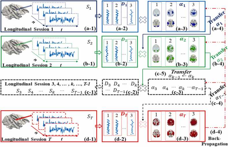 Figure 1
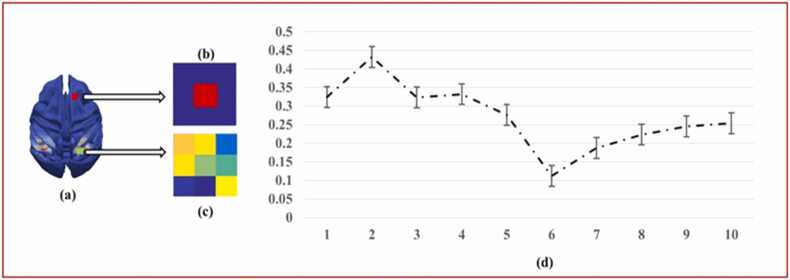 Figure 2
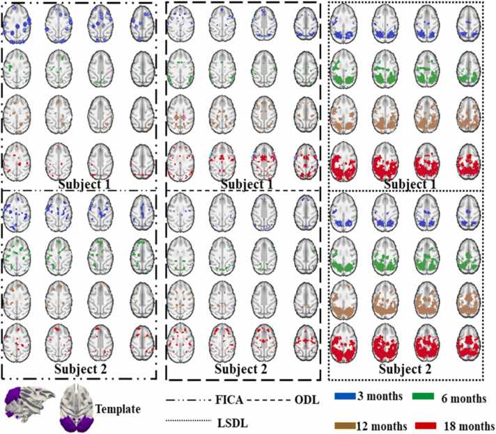 Figure 3
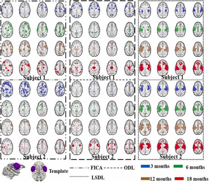 Figure 4
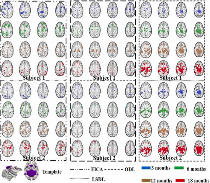 Figure 5
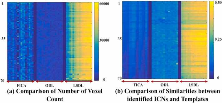 Figure 6
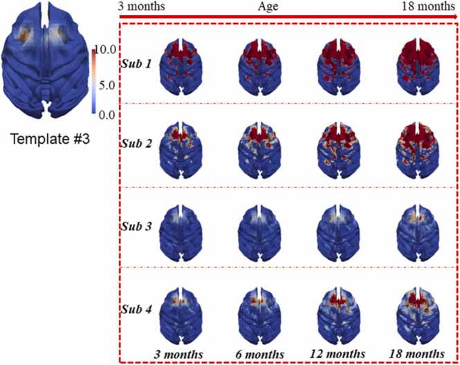 Figure 7
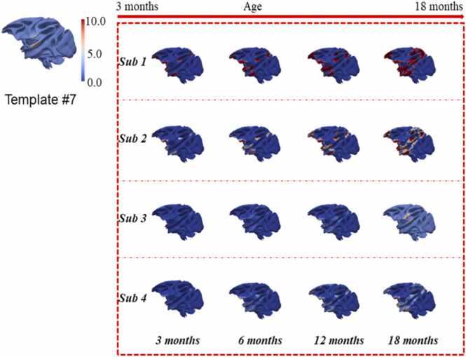 Figure 8
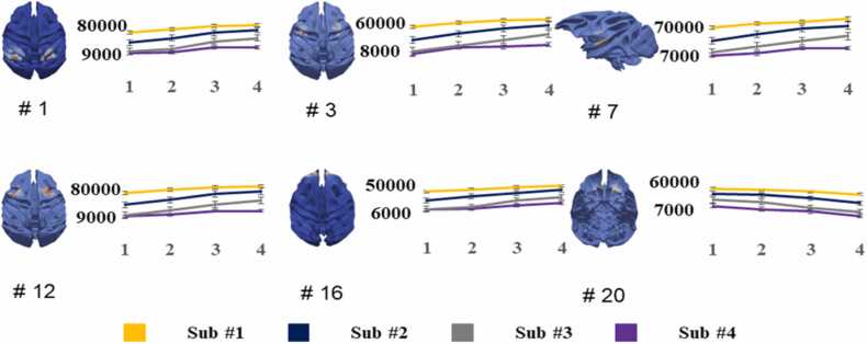 Figure 9
Peer Reviews
No public reviews on file for this paper yet. If you reviewed it on a platform where reviews are public (OpenReview, ICLR, NeurIPS, ICML), you can paste yours below so the community can read it here.
Videos
No videos yet. Explain this paper in a talk, walkthrough, or lecture? Add one.
Taxonomy
TopicsFunctional Brain Connectivity Studies · Neural dynamics and brain function · Neuroscience and Neuropharmacology Research
Introduction
1
Intrinsic Connectivity Networks (ICNs) provide insights into brain region interactions, usually depicting variations in deoxyhemoglobin concentration through functional Magnetic Resonance Imaging (fMRI) (Bullmore and Sporns, 2009, Cui et al., 2022, Fiorenzato et al., 2019, Franzmeier et al., 2019, Li et al., 2019, Peng et al., 2023, Power et al., 2011, Stam, 2014, Van Den Heuvel and Pol, 2010, Yang et al., 2022). These ICNs, denoted as spatial features from fMRI data, directly pinpoint brain regions impacted by neurological disorders more effectively than time-series analysis (Holiga et al., 2019, Ou et al., 2021, Yan et al., 2019). Notably, during the COVID-19 pandemic, researchers observed impaired ICNs in patients with olfactory loss (Wingrove et al., 2023). A vital capability of ICNs is to detect the earliest signs of impairment before irreversible structural changes occur (Lurie et al., 2020, Reid et al., 2019, Filippi et al., 2019; Agarwal et al., 2023; Kim and Ogawa, 2012, Kim and Bandettini, 2023; Ou et al., 2021; Zamani Esfahlani et al., 2020). Recent advancements in brain imaging have successfully mapped ICNs in both human and primate brains. However, several critical questions still remain: How are ICNs established during infancy and the juvenile stages? When do ICNs start to show unique functionalities distinct between juvenile and adult phases? Are the functions of specific ICNs dependent on their pre-existing connections to other brain areas? Which brain regions continue to develop through adolescence? Investigating these aspects requires examining consistent longitudinal ICNs (i.e., ICNs derived from each longitudinal fMRI dataset) across developmental stages (Deen et al., 2017, Isik et al., 2017, Kanwisher, 2017, Pereira et al., 2018).
Unfortunately, mapping consistent longitudinal ICNs at a connectome scale is inherently challenging. It requires advanced technologies to create consistent connections across ICNs over time, alongside a deep understanding of the functional complexity and even hierarchical organization of developing ICNs (Deen et al., 2017, Giedd et al., 1999, Isik et al., 2017, Kanwisher, 2017). Most current research focused on specific and localized ICNs using region-of-interest (ROI) approaches (Bachevalier, 1994, Baron-Cohen et al., 2005, Beversdorf et al., 2005, Deco et al., 2011, Goldman-Rakic and Schwartz, 1982, Herting et al., 2018, Li et al., 2019, Lipska and Weinberger, 2002), and other studies have only addressed longitudinal changes within limited ICNs or singular networks like the default mode network (DMN) (Gao et al., 2009, Sacher and Staffeldt, 1974, Van Essen et al., 2011, Van Essen et al., 2001, Van Essen, 2004).
To address these challenges, we propose an innovative method, the Longitudinal Sparse Dictionary Learning (LSDL), based on our prior work (Zhang et al., 2017, Zhang et al., 2018a, Lv et al., 2015a, Lv et al., 2015b). Overall, building on the demonstrated efficacy of Sparse Dictionary Learning (SDL) in revealing ICNs at a connectome scale via resting-state fMRI (rsfMRI), which surpasses the performance of Independent Component Analysis (ICA) (Khalilullah et al., 2023, Zhang et al., 2018a), LSDL employs a dual approach: it incorporates an additional Frobenius norm to enhance longitudinal consistency and employs Matrix Backpropagation (MBP) to mitigate potential cumulative errors (Varoquaux et al., 2011, Wytock,, Zhang et al., 2018a, Zhang et al., 2018b, Lv et al., 2017, Trigeorgis et al., 2017, Beck and Teboulle, 2009, Zhao et al., 2015, Zhao et al., 2017). In particular, the application of LSDL on longitudinal fMRI of macaque brains has successfully identified 21 consistent longitudinal ICNs. Furthermore, extensive qualitative and quantitative validations emphasize the robustness of LSDL, unveiling continuous functional developments, particularly in areas like the visual and auditory cortex. Given the structural and functional parallels between macaque and human brains, studying longitudinal ICNs in macaques can illuminate aspects of early-stage brain functional evolution (Smyser et al., 2010, Zhang et al., 2017, McCormack et al., 2015, Zhang et al., 2019a, Zhang et al., 2019b) and improve our understanding of human brain development and architecture (Isik et al., 2017, Kanwisher, 2017; Pereira et al., 2018; Zhang et al., 2017, Zhang et al., 2018a, Zhang et al., 2018b; McCormack et al., 2015).
To summarize, this work not only advances our understanding of longitudinal development within ICNs but also pave the way for investigating neurodevelopmental, neurodegenerative, and psychiatric disorders through the innovative lens of consistent longitudinal ICNs.
Methods
2
This section is structured into four main sections: 1). Computational Framework of LSDL: This sub-section delves into the details of the LSDL computational framework. It covers methodologies for identifying consistent longitudinal features and strategies for minimizing accumulative error using Matrix Backpropagation (MBP) (refer to 2.1). 2). Data Acquisition and Pre-processing: We outline the extensive data acquisition and pre-processing procedures utilized in this study, ensuring a thorough understanding of our experimental setup (refer to 2.2). 3). Parameter Tuning: This section discusses our approach to parameter tuning, specifically designed to circumvent arbitrary manual settings, enhancing the reproducibility and robustness of our findings (refer to 2.3). 4). Identification of Consistent Longitudinal ICNs: We introduce the principles underlying our methodology for identifying consistent longitudinal ICNs, emphasizing the rigor and precision of our analytical techniques (refer to 2.4). Each section aims to provide a comprehensive understanding of our methods and results, fostering clarity and facilitating replication of our research.
Longitudinal sparse dictionary learning
2.1
The computational framework of LSDL is depicted in Fig. 1. The primary innovation of LSDL lies in its capability to detect the longitudinal consistency of ICNs across various time points. Unlike traditional methods that independently analyze fMRI signals from independent time points, LSDL leverages an innovative technique entitled feature transfer to maintain the consistency in feature matrix across sequential scans. This methodology parallels the principles of deep learning (DL), where continuously transfer data is integral but can lead to cumulative errors. To address this challenge, we incorporate Matrix Backpropagation (MBP) (Gogtay et al., 2004, Zhang et al., 2017), a technique rooted in Non-negative Matrix Factorization (NMF) (Ding et al., 2005), specifically designed to minimize such errors. For a detailed explanation of this innovative approach, please refer to the legend accompanying Fig. 1.Fig. 1. Illustration of the computational framework of LSDL for modeling longitudinal macaques rsfMRI data, based on subject-level. (a-1) The rsfMRI signals of macaque brains at the first-time point are extracted and re-organized as a 2D signal matrix; (a-2) we present three examples of a learned dictionary at the first time point; (a-3) similarly, we provide corresponding three examples of learned coefficient matrix at the first time point; (a-4) all learned features are transferred to the next step; (b-1), (b-2), (b-3) and (b-4) is presented the corresponding learning steps of second time point, similarly to previous steps (a-1), (a-2), (a-3) and (a-4), respectively; (c-1) the longitudinal data set from other points, e.g., is collected and organized as 2D matrices; (c-2), (c-3) and (c-5) iteratively, we employ the model to implement the identification of longitudinal consistent features, via repeatedly transferring the learned features to the next step; represents the feature matrix learned from the previous time point and represents the current features that need to be learned; (c-4) transfer the learned feature matrix to the final stage; (d-1), (d-2) and (d-3) is presented the corresponding learning steps of final time point, similarly to previous steps (b-1), (b-2) and (b-3), respectively; (d-4) After the final feature matrix/coefficient matrix has been learned, the MBP is performed to reduce the potential accumulative errors, caused by iterative transfer of feature matrices.Fig. 1
Longitudinal feature transfer and matrix backpropagation
2.2
Consider the set of longitudinal rsfMRI signal matrices from the macaque brains, represented as , , where is the index for each time point and is the total number of rsfMRI scan sessions for each individual. In addition, n is the voxel number of whole brain space, and t represents the temporal dimension of each signal matrix, e.g., . The objective of LSDL is to decompose a dictionary matrix (i.e., weight/mixing matrix) from the initial scan session, denoted as , and a corresponding sparse coefficient matrix, denoted as :
where is the input signal matrix of rsfMRI at the first time point. In addition, represents the sparse trade-off. Eq. (1) is the same as the objective function of conventional SDL (Lv et al., 2015a, Lv et al., 2015b, Zhang et al., 2018a, Zhang et al., 2018b, Varoquaux et al., 2011). Notably, represents the number of dictionary atoms, encapsulating the dimensionality of the feature space.
Furthermore, the objective function governing other time points shown as below:
where , and , , is the input signal matrix of rsfMRI, dictionary and coefficient matrix, at time point, respectively; is the learned coefficient matrix from the last time point, transferred from the previous time point session (k-1 time point). This framework aims to decompose each signal matrix into the product of and , effectively representing each matrix as a combination of dictionary atoms and their corresponding activation patterns, which collectively constitute various ICNs. More importantly, the task involves creating a coefficient matrix that captures the essence of the ICNs over time by maintaining consistency across all temporal segments via an additional Frobenius norm, , in Eq. (2) to bridge the gap between adjacent longitudinal feature matrices, facilitating the consistent identification of ICNs. By iteratively applying Eq. (2), LSDL ensures the preservation of longitudinal consistency of the feature matrices across all time points.
Moreover, the iterative transfer the matrices can result in the potential accumulative error; to reduce the possible accumulative error, based on some previous works (Trigeorgis et al., 2017), a non-negative MBP (NMBP) is proposed:
In Eq. (3), if k is equal to final time point T, we directly set as ; otherwise, if k is smaller than T, we utilize to represent . And is denoted as ; the operator denotes the Moore-Penrose pseudo-inverse of an input matrix. is defined as the product of a series of longitudinal dictionaries as . We can update by:
where represents the selection of positive values of input matrix, and indicates the selection of negative values of input matrix.
The original MBP methods described by (3), (4) require non-negative or semi non-negative values (Trigeorgis et al., 2017). The tackling of negative values in the feature matrices, e.g., , which usually represent non-activated areas within the ICNs, presents a unique challenge for matrix-based methods that typically require non-negative values. To address this issue, we propose a novel approach where each learned coefficient matrix, e.g., , is split into positive and negative components, denoted as and , respectively. This separation allows us to conform to non-negative matrix requirements by handling the positive and absolute values of negative components distinctly. The negative components of are transformed into absolute values, noted as . Then, the MBP is applied separately to and , ensuring that the backpropagation conforms to non-negative constraints. The updated negative components are converted back to their original negative state by multiplying by −1, resulting in . This approach ensures that the integrity and representational accuracy of the original feature matrices are maintained, facilitating the preservation of essential information regarding non-activated areas within ICNs. The details of pseudo-code of proposed core algorithm are shown as below:
Core Algorithm:Longitudinal Sparse Dictionary Learning (LSDL) TableImage 1
Data acquisition and preprocessing
2.3
Rhesus macaques (Macaca mulatta) are a crucial model in neuroscience research due to their close genetic and behavioral similarities to humans (Zhang et al., 2017). This study involved four subjects from a longitudinal cohort at the Yerkes National Primate Research Center (YNPRC) at Emory University, located in Lawrenceville, Georgia. These subjects, scanned at 3, 6, 12, and 18 months of age, were part of a broader investigation into the developmental trajectories of socially raised macaques (Zhang et al., 2017, Zhang et al., 2019a). Raised in large social groups across various social hierarchies, they were nourished with a diet rich in seasonal fruits, vegetables, and high-fiber, low-fat primate chow, supplemented with enrichment items. Water was provided ad libitum. The ethical considerations of this study were rigorously maintained, adhering to the Animal Welfare Act and the U.S. Department of Health and Human Services guidelines, with approval from the Emory University Institutional Animal Care and Use Committee (IACUC) (Zhang et al., 2017, Zhang et al., 2019a). Imaging was conducted using a 3 T Siemens Trio scanner equipped with an 8-channel knee coil, at YNPRC. The macaques were anesthetized with isoflurane (0.8–1 %) to minimize the impact on functional connectivity and positioned using a customized head holder to prevent motion artifacts (Zhang et al., 2017, Zhang et al., 2018a, Zhang et al., 2019a). All were intubated and hydrated intravenously during scans and warmed with an MRI-compatible heating pad. Post-recovery, they were returned to their familial social groups.
Specifically, scanning parameters included an echo planar imaging (EPI) sequence with a repetition time (TR) of 2060 msec, an echo time (TE) of 25 msec, and a resolution of 1.5 × 1.5 × 1.5 mm^3^. Each session consisted of two 15-minute scans, yielding 400 time points per scan. Data preprocessing involved skull removal, motion correction, slice timing correction, spatial smoothing, temporal pre-whitening, global drift removal, and band-pass filtering, using FSL toolkit and in-house tools (Zhang et al., 2017, Bassett et al., 2008). The INIA19 macaque brain atlas was used as a reference for all detected ICNs, which were aligned to the atlas using FSL-FLIRT to ensure the identification of longitudinally consistent ICNs across all scans and ages (Zhang et al., 2017, Rohlfing et al., 2012). Each individual brain mask was used to extract the fMRI signals, ensuring personalized processing. The volume matrix was 85 × 104 × 65, encompassing 34,000–45,000 voxels per mask, tailored to the unique anatomical features of each subject (Zhang et al., 2017, McCormack et al., 2015).
Notably, acquiring fMRI data from animals presents unique challenges that differ significantly from human data collection (Balezeau et al., 2021). For instance, even primates cannot follow instructions as accurately as humans, often requiring anesthesia during fMRI sessions. Although the cost of raising and maintaining primates for research is exceptionally high, small sample sizes are not uncommon in impactful research involving non-human primates (Nakahara et al., 2002, Nelissen and Vanduffel, 2011).
Hyperparameter and parameter tuning
2.4
To optimally determine crucial parameters in LSDL, such as dictionary size, sparse trade-off, and parameters controlling the similarity between adjacent coefficient matrices, we utilize multiple techniques for parameter tuning, guided by our previous research (Zhang et al., 2017, Zhang et al., 2019a). Initially, we utilize a technique known as the rank estimator to determine the dictionary size. This rank estimator (Zhang et al., 2017, Varoquaux et al., 2011, Liu et al., 2010) advances the determination of potentially optimal dictionary size, which corresponds to the input dictionary size used in the LASSO (Lv et al., 2015a, Lv et al., 2015b, Lv et al., 2017, Zhang et al., 2017, Zhang et al., 2018a). This approach involves accurately estimating the rank of each individual fMRI signal matrix, which informs the dictionary size and ensures the adequacy to capture the inherent complexity of the input data such as . The rank estimator utilizes a rank-revealing method based on Orthogonal Decomposition, specifically QR factorization (Katsikis et al., 2021, Wen et al., 2012). Initially, the method determines the estimated rank of each signal matrix . This initial rank helps guide the iterative calculation to find the optimal rank for the input matrix. If the initial estimated rank is found to be larger than the optimal rank, the algorithm examines the diagonal elements of the upper-triangular matrix resulting from the QR factorization of (Wen et al., 2012). This step is crucial to ensure that any redundancy in the data representation is minimized, thus enhancing the sparsity and effectiveness of the dictionary learning process.
In addition, we can confirm the optimal size of through QR factorization. During this phase, the magnitudes of the diagonal elements of should ideally show a non-increasing trend (Katsikis et al., 2021). This condition indicates that the matrix dimensions are correctly estimated, optimizing the computational efficiency and accuracy of the model. To finalize the rank determination, the algorithm employs thresholding values specified in Eqs. (5) and (6), which solidify the rank decision by establishing clear cutoffs (Liu et al., 2010) based on the matrix's diagonal line, denoted as . From this diagonal, and are computed to quantitatively describe the rank structure of . These vectors assist in the final determination of the dictionary size and composition, ensuring that the learned features are both representative and efficient in capturing the underlying patterns of the fMRI data.
and then examine the value:
where is the maximum element of the vector (with the largest index p if the maximum value is not unique). In our current implementation, we reset the rank estimated r top once , and this adjustment can be successfully done only once (Katsikis et al., 2021). By using the rank-revealing, we can set the initial number of components, i.e., ICNs, the same as input matrix, e.g., 400.
Moreover, another important parameter denoted as the sparse trade-off can be estimated via Rose algorithm. According to the theoretical research, we aim to optimize the selection of a crucial parameter , that is the sparse trade-off. Based on the theorem in research works, if assume to be 0, we have an equivalent format of a min-max problem, e.g., dual format for a single time points of Eq. (4) here:
The linear system can be organized as:
Eq. (8) has a unique solution, denoted by . Let
Using the Rose algorithm provided in [41], let be the Hessian matrix, and then we can estimate the maximal value of . An attenuation series has been introduced in the literature (Liu et al., 2010) as that is adopted to determine the value of , i.e., , , and . Therefore, we set . By the estimation using Eq. (9), we have .
Furthermore, to empirically determine the parameter which controls the similarity between features from adjacent time points, we conduct an experiment spanning a range of values from 0.1 to 1.0. Our method involves analyzing all voxels within the identified coefficient matrices, which represent the ICNs or feature matrices. Specifically, we categorize voxels into two categories based on their contribution to the signal quality: noisy voxels and meaningful voxels. Noisy voxels are identified through Eq. (10), which likely include background noise or non-neuronal fluctuations. Conversely, meaningful voxels, representing significant neural activity, are identified using Eq. (11) and are visually represented by red squares in Fig. 2. This distinction is critical for evaluating the quality and reliability of the ICNs extracted by our method. Specifically, two categorizations of voxels construct two corresponding sets, and the mathematic description is:
where represents a given open cube, and radius (Wheeden, 2015); for , is denoted as the center of the given cube (Mantini et al., 2013). By examining the ratio of two kinds of voxels, the optimal can be decided in this study. The following figure briefly describe the method to determine the parameter .Fig. 2. The description of framework for our proposed method on identification of threshold to binarize identified ICNs. (a) an identified ICN from coefficient matrix is visualized, and two different voxels denoted via (10), (11) are presented as red, green square, respectively; (b) an example of the noisy voxel, represented as in Eq. (10), is described as a red square, and its surrounding area is empty; (c) an example of meaningful voxel, denoted as Eq. (11), is shown as the central green square and its neighbor voxels are non-zero; (d) we calculate the average ratio between these two kinds of voxels, based on the identified ICNs extracted from the coefficient matrices of all subjects; the numbers of 1–10 represent the corresponding value of , from 0.1 to 1.0; obviously, the 0.60 is the optimal value for , which can provide the less noisy voxels.Fig. 2
Moreover, to further eliminate arbitrary within identified ICNs via LSDL, Fast Independent Component Analysis (FICA) (Calhoun et al., 2001, Khalilullah et al., 2023), and Online Dictionary Learning (ODL) (Lv et al., 2015a, Lv et al., 2015b), we standardize all intensities of identified ICNs using Z-score. Specifically, we convert these intensities into Z-scores, following the methodologies described in (Zhang et al., 2017, Zhang et al., 2018a, Lv et al., 2015a, Lv et al., 2015b, Varoquaux et al., 2011). These Z-scores are then binarized to facilitate voxel counting, which is a critical step in our subsequent validation processes.
Besides, we propose a novel voxel count technique, which is a crucial metric for assessing longitudinal variations across different time sessions (Lv et al., 2015a, Lv et al., 2015b, Howell et al., 2016, Caviness et al., 1996). In particular, the voxel count technique comprehensively considers adjacent voxels’ intensity and determines the threshold to facilitate the calculation of area, e.g., the number of voxels, in each identified ICN. Benefitting from voxel count, we can differentiate the variation of area in each ICN.
The principle to detect consistent longitudinal ICNs in macaque brain
2.5
In our prior studies (Zhang et al., 2017, Zhang et al., 2018a; Zhang et al., 2019a, 2019b), we have effectively documented 70 intrinsic connectivity network (ICN) templates for the macaque brain. Additionally, we provide individual longitudinal ICNs corresponding to these templates, enhancing our understanding of their consistent longitudinal development. We employed ICA, SDL, and LSDL, following recommended parameters (Lv et al., 2015a, Lv et al., 2015b, Lv et al., 2017, Zhang et al., 2017, Zhang et al., 2018a, Zhang et al., 2018b; Beck and Teboulle, 2009, Varoquaux et al., 2011, Wytock,), to detect longitudinally consistent ICNs. Specifically, FICA (Calhoun et al., 2001, Khalilullah et al., 2023) utilizes a single vital parameter—the number of potential independent components—to automatically estimate parameters and determine the number of components. For ODL, Lv et al. recommended parameters include a dictionary size of 400 and a sparse trade-off of 0.15 (Lv et al., 2015a, Lv et al., 2015b, Lv et al., 2017).
Our rigorous principle for determining longitudinal consistency ensures that all identified ICNs across all time points exhibit monotonous variance. We define monotonicity qualitatively, where the regions of an ICN should expand beyond those identified in previous time points, aligning with adolescent neural developments (Deen et al., 2017, Isik et al., 2017, Kanwisher, 2017, Pereira et al., 2018, Malkova et al., 2006, Knickmeyer et al., 2008, Knickmeyer et al., 2010, Machado and Bachevalier, 2003). Quantitatively, the voxel count within an ICN should consistently increase across time points, using a predetermined threshold (Malkova et al., 2006, Knickmeyer et al., 2008, Knickmeyer et al., 2010, Machado and Bachevalier, 2003).
In the following sections, we present and examine results based on these qualitative and quantitative criteria. Using prior research (McCormack et al., 2015, Zhang et al., 2017), we align identified ICNs via FICA, ODL, and LSDL with established macaque brain ICN templates (Machado and Bachevalier, 2003, McCormack et al., 2015, Zhang et al., 2017; Bosman et al., 2012). This alignment uses our rigorous principle to pinpoint potential longitudinally consistent ICNs. We offer a comprehensive qualitative presentation to validate the three methods' performance, focusing on longitudinal consistency, supplemented by an overarching quantitative analysis to affirm the methods' efficacy. Further details and explanations are provided in the subsequent sections.
Results
3
We employ two different computational frameworks: ME-ICA & DELMAR versus DELMAR/Denoise/Mapping to investigate the hierarchical organization of BCNs and their reproducibility from MBME fMRI. As discussed, in following sections, we hope to prove multiple hypotheses raised in the Introduction section.
Experimental comparison of LSDL with FICA and SDL
3.1
To validate the efficacy of the proposed LSDL, we conducted comparative analyses using two representative peer methods: FICA and ODL (Calhoun et al., 2001; Khalilullah et al., 2023; Lv et al., 2015a, Lv et al., 2015b, Lv et al., 2017). These methods are widely recognized as efficient, data-driven approaches for modeling fMRI signals (Zhang et al., 2017, Vanduffel et al., 2014, Miyamoto et al., 2013, Nakahara et al., 2002, Nelissen et al., 2005, Nelissen and Vanduffel, 2011). Utilizing the recommended parameters from prior research (Zhang et al., 2017, Zhang et al., 2018a, Zhang et al., 2018b Miyamoto et al., 2013; Nakahara et al., 2002), we applied FICA and ODL to perform identical ICN identifications. Our previous study (Zhang et al., 2017, Zhang et al., 2018a, Zhang et al., 2019a) have documented 70 ICN templates at the connectome scale for macaque brains. Initially, we aligned the ICNs identified by FICA, ODL, and LSDL with these previously identified templates. Given that LSDL is specifically designed to detect longitudinally consistent features, we implemented a rigorous validation framework to assess the longitudinal trajectories of ICNs and compare the effectiveness of the three methods. This evaluation framework aims to highlight the robustness of LSDL in maintaining longitudinal consistency across multiple temporal stages. In the ensuing figures, we present a qualitative comparison of the three methodologies using three illustrative templates: the visual area, auditory area, and the Default Mode Network (DMN). These comparisons are intended to demonstrate the distinct capabilities of each method in capturing and consistently tracking the dynamic changes within specific ICNs over time in Fig. 3, Fig. 4, Fig. 5.Fig. 3. This figure provides a qualitative comparison from two subjects of ICA, ODL and LSDL based on the identified template of visual area (Zhang et al., 2017, Miyamoto et al., 2013, Nakahara et al., 2002, Nelissen et al., 2005, Nelissen and Vanduffel, 2011). The different dash lines represent the results obtained by different methods. And different colors represent the identified ICNs from different time points. By qualitative observation, the results from LSDL demonstrate the longitudinal consistency. The activation regions of ICNs are becoming larger and stronger through all time points. However, the ICNs identified via FICA and ODL are not very consistent. The identified ICNs are varied from initial time points to the final time points. Obviously, for example, some identified ICNs via ICA and ODL, occupy the larger brain regions, but some revealed regions become smaller at the final stage.Fig. 3. Fig. 4This figure provides a qualitative comparison from two subjects of ICA, ODL, and LSDL based on the identified template of auditory area (Zhang et al., 2017, Miyamoto et al., 2013, Nakahara et al., 2002, Nelissen et al., 2005, Nelissen and Vanduffel, 2011). By qualitative observation, the results from LSDL demonstrate the longitudinal consistency. The notations are the same or similar as those discussed in Fig. 3. Similarly, it is easy to observe the longitudinal consistent ICNs identified by LSDL. Meanwhile, both FICA and ODL cannot successfully identify the longitudinal consistent features. And the ICNs obtained by LSDL demonstrate that the monotonous development of longitudinal ICNs which also satisfy the reports of juvenile developmental brains (Zhang et al., 2017, Miyamoto et al., 2013, Nakahara et al., 2002, Nelissen et al., 2005, Nelissen and Vanduffel, 2011).Fig. 4. Fig. 5This figure provides the qualitative comparison from two subjects of ICA, ODL and LSDL based on the identified template of DMN (Zhang et al., 2017, Zhang et al., 2018a, Zhang et al., 2018b). The notations are the same or similar as those discussed in Fig. 3. Like other qualitative examples, the identified longitudinal DMNs via LSDL are gradually stronger than previous time points. However, the results obtained by FICA and ODL cannot successfully demonstrate the longitudinal consistency/monotonicity.Fig. 5
In addition, following the presentation of the three examples, we offer additional qualitative comparisons through detailed visualizations and slices of identified ICNs, using the different methodologies applied. Below are links to the visual outputs for each method, providing a deeper insight into the ICNs identified in the four macaque subjects:
Moreover, for further qualitative comparison using ODL method, here are the links showcasing the ICNs identified in the four macaque subjects involved in our study:
Besides, for a thorough qualitative comparison using the LSDL method, here are the links showcasing the ICNs identified in the four macaque subjects involved in our study:
Lastly, to further validate the proposed LSDL method, we conducted ten independent trials for each method, such as FICA, ODL, and LSDL to ensure a consistent quantitative comparison. The results are graphically presented in Fig. 6, which comprises several parts detailing our findings. In particular, Fig. 6(a) showcases the longitudinal voxel count analysis. To standardize measurements and avoid arbitrary comparisons, all identified ICNs were converted into Z-scores as per protocols in references (Zhang et al., 2017, Zhang et al., 2018a, Zhang et al., 2019a, Lv et al., 2017). We then applied a threshold of 0.10 (Zhang et al., 2017, Zhang et al., 2018a, Zhang et al., 2019a, Lv et al., 2017) to count the number of voxels for each identified ICN. These voxel counts, organized from ages 3 months to 18 months across all subjects, demonstrate a consistent increase in voxel numbers over time with LSDL, indicating robust feature detection. In contrast, the voxel counts from ICAs and ODL varied significantly, lacking a clear pattern of consistency or monotonic increase. Meanwhile, Fig. 6(b) utilized the Hausdorff metric (Zhang et al., 2017) to evaluate the similarity between the identified longitudinal ICNs and predefined templates. The similarities, arranged by columns for each age from 3 to 18 months, showed increasing congruence over time when using LSDL, affirming its effectiveness in tracking longitudinal development. This pattern was not as pronounced with FICA, and ODL exhibited significant longitudinal variations, with FICA showing a peculiar peak in similarity at the second time point only. Importantly, we leverage techniques such as voxel counting, which allows us to quantify the number of voxels that surpass a defined threshold (illustrated in Fig. 6(a)), and spatial similarity metrics (illustrated in Fig. 6(b)) that align the identified individual ICNs with established templates (Zhang et al., 2017). These quantitative methods offer robust, precise insights, even in smaller-scale studies, making them particularly well-suited to our investigation. By employing these approaches, we can efficiently and effectively validate the individual ICNs without the need for large, resource-intensive datasets (Zhang et al., 2017). To summarize, these results clearly highlight the advanced capability of LSDL in identifying robust and consistent ICNs longitudinally, compared to the traditional methods of FICA and ODL. The results further reinforce LSDL as an advanced technology in longitudinal brain connectivity studies.Fig. 6. The overall and comprehensive quantitative comparison of ICA, ODL, and LSDL, based on 10 repeated experiments. These two subfigures (a) and (b) present the quantitative analyses of longitudinal voxel count, shown in (a) as well as the similarities between each identified ICNs and original templates, presented in (b). For subfigures (a) and (b), each column represents the corresponding average result calculated from a single time point from a macaque subject; all time points are organized from 3 months to 18 months. Obviously, by the observation, the results achieved by LSDL demonstrate the efficient performance to identify the longitudinal consistent ICNs from 3 months to 18 months, presented from the left to the right column.Fig. 6
Identified consistent longitudinal ICNs in macaque brains
3.2
In this section, we present 21 consistent longitudinal ICNs via LSDL. These ICNs showcase changes in activation intensity across developmental stages, indicating either intensification or diminution relative to earlier time points. This observation confirms our method's ability to capture the dynamic evolution of ICNs across different ages in macaques.
Notably, the effectiveness of LSDL in mapping these changes provides substantial evidence concerning the developmental trajectory of juvenile primate brains. Primarily, our findings contribute significantly to understanding how primates rely on their visual and auditory systems for environmental interaction, which aligns with numerous prior studies that have focused on the visual cortex and related neural networks (Howell et al., 2016, Knickmeyer et al., 2010, McCormack et al., 2015; Mantini et al., 2011). The following Fig. 7, Fig. 8 demonstrate two examples of 21 consistent longitudinal ICNs identified via LSDL.Fig. 7. The presentation of an example of longitudinal consistent ICN #3, via mapping the detected ICNs to the cortical surface of macaque brain, to provide an overall qualitative observation; by the mapping to the surface, it is easier to observe the longitudinal developments of juvenile ICNs of macaques; the regions mapped to the cortical surface of ICNs is enlarging through all time points.Fig. 7. Fig. 8The presentation of another example of longitudinal consistent ICN #7, via mapping the detected spatial networks to the cortical surface of macaque, to provide an overall observation; it is obvious to observe the longitudinal developments of juvenile ICNs of macaques; the regions mapped to the cortical surface of ICNs is developing through all time points.Fig. 8
In addition, more details and slices of identified 21 consistent longitudinal ICNs across 4 macaques can be viewed by our website as follow:
Furthermore, for further quantitative validation of the 21 identified longitudinal consistent ICNs, we have conducted extensive quantitative analytics using voxel count on each ICN.
Overall, Fig. 9 illustrates a detailed quantitative analysis of six representative consistent longitudinal ICNs, highlighting changes in voxel counts from 3 to 18 months. The voxel count, a measure of activated voxels within each network, offers a precise indication of the changes in the area of each ICN over time. Specifically, the results reveal a consistent increase in the voxel count for ICNs #1, #3, #7, #12, and #16. This growth suggests a continuous expansion in the areas of the brain these ICNs cover, reflecting potentially significant developmental processes. The increase in voxel count indicates not just more extensive neural engagement within these networks but may also imply enhancements in functions associated with these areas, such as sensory integration, cognitive processing, and social interaction skills. In contrast, ICN #20 exhibits a gradual reduction in voxel count throughout the observed periods. This decline could indicate a process of synaptic pruning, where less efficient or less necessary neural connections are eliminated, potentially leading to a more efficient and specialized brain network. The consistent decrease in this network's area warrants further investigation to understand the developmental implications and underlying mechanisms. The contrasting trajectories observed among these ICNs underscore the dynamic and complex nature of brain development during early childhood. Notably, the reduction in ICN #20, amidst the growth observed in other networks, highlights an intriguing area for further research. Future studies should aim to include a larger cohort of macaques to validate these findings and explore the functional consequences of these developmental changes. Notably, ICNs, which represent the interaction between activated brain regions, typically reflect variations in deoxyhemoglobin concentration in rsfMRI data (Cui et al., 2022, Fiorenzato et al., 2019, Franzmeier et al., 2019). Consequently, the intensity for each individual reflects the specific activation levels within functional brain areas (Li et al., 2019, Peng et al., 2023, Yang et al., 2022). Given the uniqueness of each animal, the variation in intensity across individuals highlights these inherent differences.Fig. 9. It illustrates a quantitative analysis of six representative ICNs, identified across four developmental stages: 3, 6, 12, and 18 months. These stages are denoted as Time Points 1, 2, 3, and 4, respectively. The analysis employs voxel count as a metric to measure the longitudinal variance within each ICN, offering insights into their developmental trajectories over time.Fig. 9
Moreover, the detailed quantitative results and visualizations of this analysis can be accessed through our dedicated webpage:
On the dedicated webpage, we display representative slices of the corresponding ICN templates and the longitudinal voxel count data for the four macaque subjects involved in our experiments. Each subject is represented by a different color for clarity. Generally, the voxel counts of the longitudinal consistent ICNs show a continuous increase through all assessed time points, from 3 months to 18 months. This linear increase in voxel counts aligns with the developmental patterns reported in the research works by Machado, Malkova, and Knickmeyer (Howell et al., 2016, Knickmeyer et al., 2010, Machado and Bachevalier, 2003; Zhang et al., 2017; McCormack et al., 2015). The quantitative results effectively illustrate the linear variance, further validating the reliability and consistency of our findings in the developmental trajectory of these ICNs.
To summarize, these quantitative analyses not only provide valuable insights into the functional dynamics of early brain development but also set the stage for deeper explorations into how these changes impact overall brain function and development. Understanding these consistent and dynamic patterns is crucial for advancing our knowledge of neurological development and could have implications for early diagnosis and intervention in developmental disorders.
Discussion
4
In this work, we introduced an innovative LSDL method, specifically designed to unearth consistent longitudinal ICNs within macaque brains using functional MRI data collected over time. Through meticulous validation, LSDL has proven its superior efficacy by successfully identifying 21 consistent longitudinal ICNs, outperforming traditional methods such as FICA and ODL.
Overall, the effectiveness of LSDL was rigorously validated against several peer-reviewed methods, clearly demonstrating its superior ability to detect consistent longitudinal features—namely, ICNs. This not only underscores the robustness of LSDL but also showcases its potential to significantly advance research in critical areas such as adolescent neuroscience and developmental brain studies. The precision of LSDL paved the way for an in-depth investigation of functional developments in specific brain regions, thereby enhancing the accuracy and reliability of longitudinal studies.
In addition, our research extends beyond individual findings to encompass extensive comparative studies between adolescent primates and human infants, focusing on crucial areas like the visual cortex, auditory regions, and the Default Mode Network (DMN). These studies illuminate the similarities and differences in developmental patterns between species, enriched by the longitudinally consistent networks that LSDL identifies. Such insights are instrumental in understanding developmental trajectories and contribute profoundly to advanced comparative neuroscientific research.
Moreover, the consistent networks identified by LSDL can be integrated with a diverse array of biological data, including genetic, protein, connectivity, and anatomical information. This holistic approach is pivotal for refining the publicly available macaque longitudinal cortical parcellation atlas. It also pushes the boundaries of our understanding of brain development across different species, suggesting a comprehensive model of brain evolution that is deeply rooted in empirical evidence.
This study not only highlights the utility of the LSDL method in tracing and understanding longitudinal brain development but also sets a robust foundation for future explorations into the dynamic changes occurring in the brain from infancy through adulthood. By providing a sophisticated framework to reveal consistent longitudinal ICNs, LSDL significantly enhances our ability to decipher complex neurological trajectories and their implications for health and disease. Future research will leverage this advanced methodology to explore further the intricate processes underlying brain development and its disorders, opening new frontiers in neuroscience and clinical applications.
Ethical approval
This study involved four subjects from a longitudinal cohort at the Yerkes National Primate Research Center (YNPRC) at Emory University, located in Lawrenceville, Georgia. Notably, the ethical considerations of this study were rigorously maintained, adhering to the Animal Welfare Act and the U.S. Department of Health and Human Services guidelines, with approval from the Emory University Institutional Animal Care and Use Committee (IACUC).
Confidentiality
Participant confidentiality will be strictly maintained throughout the study. Data will be accessible only to the research team and will be used solely for the purposes of this study.
Data protection
All data will be collected, stored, and processed in accordance with the relevant data protection laws and regulations, such as the General Data Protection Regulation (GDPR). Data will be securely stored in encrypted files and protected databases.
Risk minimization
The study will be designed to minimize any potential risks to participants. Any foreseeable risks will be clearly communicated to the participants, and appropriate measures will be taken to mitigate these risks. In the event of any adverse effects, appropriate support and intervention will be provided.
Conclusion
This statement reaffirms our commitment to conducting the proposed research with the highest ethical standards. We will ensure that all procedures are carried out with respect for the rights, dignity, and well-being of the participants.
Conflict of interest and compliance with ethical standards
This Ethics Statement outlines the conflict of interest and ethical considerations and procedures that will be adhered to in the proposed research project. The study aims to 1). Propose and validate an effective Longitudinal Sparse Dictionary Leaning (LSDL) for fMRI cohorts’ analytics; 2). Present multiple consistent longitudinal intrinsic connectivity networks (ICNs) Ensuring the highest standards of ethical conduct is paramount throughout this research process.
CRediT authorship contribution statement
Wei Zhang: Validation, Supervision, Resources, Methodology, Investigation, Funding acquisition, Data curation, Conceptualization. Yu Bao: Validation, Formal analysis. Afrar Jahin: Writing – review & editing, Writing – original draft, Conceptualization. Arif Hassan Zidan: Writing – review & editing, Writing – original draft.
Conflict of Interest
All authors have no conflicts of interest to disclose.
The reference list from the paper itself. Each links out to its DOI / PubMed record.
- 1Agarwal S.Al Khalifah H.Zaca D.Pillai J.J.f MRI and DTI: review of complementary techniques Funct. Neuroradiol. Princ. Clin. Appl.202310251060
- 2Bachevalier J.Medial temporal lobe structures and autism: a review of clinical and experimental findings Neuropsychologia 3261994627648808442010.1016/0028-3932(94)90025-6 · doi ↗ · pubmed ↗
- 3Balezeau F.Nacef J.Kikuchi Y.Schneider F.Rocchi F.Muers R.S.Murphy K.MRI monitoring of macaque monkeys in neuroscience: case studies, resource and normative data comparisons Neuro Image 230202111777810.1016/j.neuroimage.2021.117778 PMC 806318233497775 · doi ↗ · pubmed ↗
- 4Bosman C.A.Schoffelen J.M.Brunet N.Oostenveld R.Bastos A.M.Womelsdorf T.Rubehn B.Stieglitz T.De Weerd P.Fries P.Attentional stimulus selection through selective synchronization between monkey visual areas Neuron 7520128758882295882710.1016/j.neuron.2012.06.037PMC 3457649 · doi ↗ · pubmed ↗
- 5Baron-Cohen S.Knickmeyer R.C.Belmonte M.K.Sex differences in the brain: implications for explaining autism Science 310574920058198231627211510.1126/science.1115455 · doi ↗ · pubmed ↗
- 6Bassett D.S.Hierarchical organization of human cortical networks in health and schizophrenia J. Neurosci.28372008923992481878430410.1523/JNEUROSCI.1929-08.2008 PMC 2878961 · doi ↗ · pubmed ↗
- 7Beck A.Teboulle M.A fast iterative shrinkage-thresholding algorithm for linear inverse problems SIAM J. Imaging Sci.212009183202
- 8Beversdorf D.Q.Manning S.E.Hillier A.Anderson S.L.Nordgren R.E.Walters S.E.Bauman M.L.Timing of prenatal stressors and autism J. Autism Dev. Disord.35420054714781613403210.1007/s 10803-005-5037-8 · doi ↗ · pubmed ↗