Nonparametric Bayesian Adjustment of Unmeasured Confounders in Cox Proportional Hazards Models
Shunichiro Orihara, Shonosuke Sugasawa, Tomohiro Ohigashi, Keita Hirano, Tomoyuki Nakagawa, Masataka Taguri

TL;DR
This paper introduces a new Bayesian method to adjust for unmeasured confounders in survival analysis, improving accuracy without relying on traditional assumptions.
Contribution
A novel nonparametric Bayesian procedure is introduced to estimate hazard ratios while addressing limitations of existing methods.
Findings
The proposed Bayesian procedure outperforms existing methods in some performance metrics.
The method accurately identifies cluster structures and achieves statistical efficiency comparable to efficient estimators.
Abstract
Unmeasured confounders pose a major challenge in accurately estimating causal effects in observational studies. To address this issue when estimating hazard ratios (HRs) using Cox proportional hazards models, several methods, including instrumental variables (IVs) approaches, have been proposed. However, these methods often face limitations, such as weak IV problems and restrictive assumptions regarding unmeasured confounder distributions. In this study, we introduce a novel nonparametric Bayesian procedure that provides accurate HR estimates while addressing these limitations. A key assumption of our approach is that unmeasured confounders exhibit a cluster structure. Under this assumption, we integrate two remarkable Bayesian techniques, the Dirichlet process mixture (DPM) and general Bayes (GB), to simultaneously (1) detect latent clusters based on the likelihood of exposure and…
Genes, proteins, chemicals, diseases, species, mutations and cell lines named across the full text — each resolved to its canonical identifier and authoritative record.
Click any figure to enlarge with its caption.
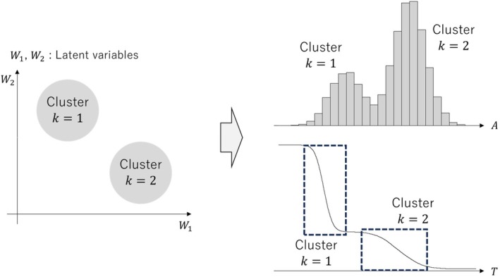 FIGURE 1
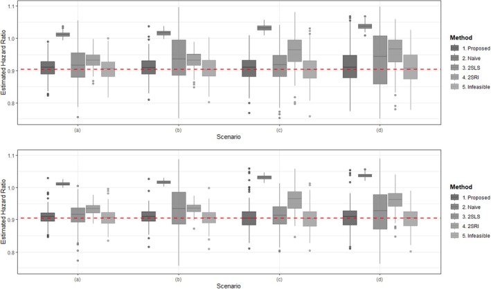 FIGURE 2
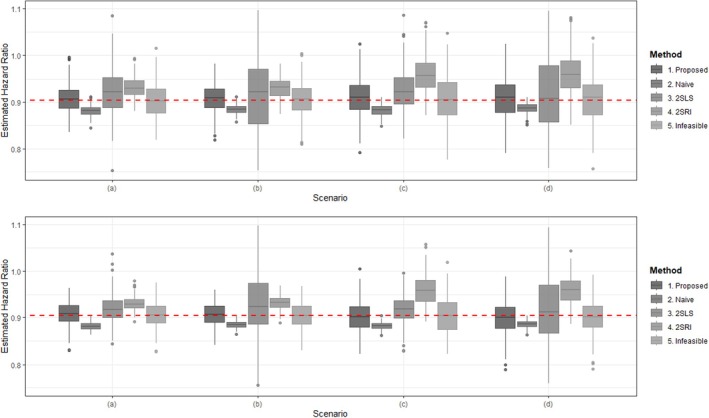 FIGURE 3
| log–hazard ratio | ||||||||||
|---|---|---|---|---|---|---|---|---|---|---|
| Setting | Scenario | Method | Bias | ESE | RMSE | CP | Bias | ESE | RMSE | CP |
| Easy to identify | (a) | 1. Proposed | 0.004 | 0.034 | 0.034 | 0.985 | 0.004 | 0.028 | 0.028 | 0.975 |
| 2. Naive | 0.111 | 0.008 | 0.112 | 0.000 | 0.111 | 0.006 | 0.111 | 0.000 | ||
| 3. 2SLS | −0.014 | 0.266 | 0.267 | 0.855 | 0.007 | 0.042 | 0.043 | 0.875 | ||
| 4. 2SRI | 0.031 | 0.026 | 0.040 | 0.680 | 0.031 | 0.017 | 0.035 | 0.505 | ||
| 5. Infeasible | 0.000 | 0.040 | 0.040 | 0.955 | 0.001 | 0.029 | 0.029 | 0.945 | ||
| (b) | 1. Proposed | 0.005 | 0.037 | 0.037 | 0.975 | 0.005 | 0.029 | 0.029 | 0.970 | |
| 2. Naive | 0.116 | 0.007 | 0.116 | 0.000 | 0.116 | 0.005 | 0.116 | 0.000 | ||
| 3. 2SLS | −0.548 | 6.477 | 6.500 | 0.835 | 0.055 | 1.292 | 1.293 | 0.880 | ||
| 4. 2SRI | 0.029 | 0.028 | 0.041 | 0.650 | 0.032 | 0.016 | 0.036 | 0.445 | ||
| 5. Infeasible | 0.000 | 0.040 | 0.040 | 0.955 | 0.001 | 0.030 | 0.030 | 0.940 | ||
| (c) | 1. Proposed | 0.004 | 0.045 | 0.045 | 0.985 | 0.002 | 0.044 | 0.044 | 0.940 | |
| 2. Naive | 0.131 | 0.009 | 0.132 | 0.000 | 0.131 | 0.006 | 0.131 | 0.000 | ||
| 3. 2SLS | 0.008 | 0.057 | 0.057 | 0.890 | 0.007 | 0.040 | 0.041 | 0.875 | ||
| 4. 2SRI | 0.060 | 0.055 | 0.082 | 0.680 | 0.060 | 0.037 | 0.071 | 0.475 | ||
| 5. Infeasible | 0.001 | 0.051 | 0.051 | 0.945 | −0.002 | 0.039 | 0.039 | 0.950 | ||
| (d) | 1. Proposed | 0.005 | 0.057 | 0.057 | 0.960 | 0.002 | 0.044 | 0.044 | 0.935 | |
| 2. Naive | 0.137 | 0.009 | 0.137 | 0.000 | 0.136 | 0.006 | 0.137 | 0.000 | ||
| 3. 2SLS | 0.276 | 3.211 | 3.222 | 0.860 | 0.057 | 1.533 | 1.534 | 0.880 | ||
| 4. 2SRI | 0.058 | 0.056 | 0.081 | 0.640 | 0.059 | 0.036 | 0.070 | 0.500 | ||
| 5. Infeasible | 0.003 | 0.056 | 0.056 | 0.950 | −0.001 | 0.038 | 0.038 | 0.950 | ||
| Hard to identify | (a) | 1. Proposed | 0.004 | 0.034 | 0.034 | 0.985 | 0.003 | 0.027 | 0.027 | 0.985 |
| 2. Naive | −0.026 | 0.012 | 0.029 | 0.445 | −0.027 | 0.009 | 0.028 | 0.105 | ||
| 3. 2SLS | 0.016 | 0.051 | 0.054 | 0.950 | 0.016 | 0.034 | 0.037 | 0.935 | ||
| 4. 2SRI | 0.029 | 0.023 | 0.037 | 0.765 | 0.027 | 0.015 | 0.032 | 0.675 | ||
| 5. Infeasible | −0.002 | 0.042 | 0.042 | 0.970 | 0.001 | 0.030 | 0.030 | 0.965 | ||
| (b) | 1. Proposed | 0.003 | 0.036 | 0.036 | 0.995 | 0.002 | 0.028 | 0.028 | 0.975 | |
| 2. Naive | −0.022 | 0.011 | 0.025 | 0.495 | −0.022 | 0.008 | 0.024 | 0.220 | ||
| 3. 2SLS | 4.689 | 66.751 | 66.915 | 0.970 | 0.034 | 0.250 | 0.253 | 0.935 | ||
| 4. 2SRI | 0.028 | 0.023 | 0.037 | 0.750 | 0.029 | 0.016 | 0.033 | 0.525 | ||
| 5. Infeasible | −0.001 | 0.041 | 0.041 | 0.950 | 0.000 | 0.030 | 0.030 | 0.970 | ||
| (c) | 1. Proposed | 0.006 | 0.046 | 0.046 | 0.990 | −0.004 | 0.036 | 0.036 | 0.980 | |
| 2. Naive | −0.025 | 0.013 | 0.028 | 0.535 | −0.026 | 0.009 | 0.027 | 0.165 | ||
| 3. 2SLS | 0.018 | 0.048 | 0.052 | 0.930 | 0.015 | 0.033 | 0.036 | 0.905 | ||
| 4. 2SRI | 0.061 | 0.047 | 0.077 | 0.720 | 0.058 | 0.032 | 0.066 | 0.540 | ||
| 5. Infeasible | 0.003 | 0.055 | 0.055 | 0.960 | −0.001 | 0.040 | 0.040 | 0.970 | ||
| (d) | 1. Proposed | 0.002 | 0.050 | 0.050 | 0.985 | −0.006 | 0.039 | 0.039 | 0.975 | |
| 2. Naive | −0.020 | 0.012 | 0.024 | 0.665 | −0.021 | 0.009 | 0.023 | 0.345 | ||
| 3. 2SLS | −0.101 | 1.727 | 1.730 | 0.960 | 0.005 | 0.133 | 0.133 | 0.935 | ||
| 4. 2SRI | 0.061 | 0.048 | 0.077 | 0.690 | 0.058 | 0.030 | 0.066 | 0.500 | ||
| 5. Infeasible | 0.001 | 0.055 | 0.055 | 0.945 | −0.004 | 0.039 | 0.039 | 0.960 | ||
| Methods | Point estimate (95% CI) |
|---|---|
| CPHM (No adjustment) | |
| CPHM (Age and sex) | |
| CPHM (Age, sex, smoking and drinking habits) | |
| 2SLS | |
| 2SRI | |
| Proposed |
| Group | |||
|---|---|---|---|
| Health‐unconscious | Health‐conscious | ||
| Parameter | SMD | ||
| Age | 56.4 (8.0) | 56.8 (7.9) | 0.050 |
| Sex | 13341 (44.4%) | 833 (40.8%) | 0.073 |
| Smoking habits | 2173 (7.2%) | 102 (5.0%) | 0.092 |
| Drinking habits | 28218 (94.0%) | 1845 (90.3%) | 0.138 |
| Sleeping status | 1951 (19.4%) | 153 (23.4%) | 0.098 |
- —Japan Society for the Promotion of Science10.13039/501100001691
Peer Reviews
No public reviews on file for this paper yet. If you reviewed it on a platform where reviews are public (OpenReview, ICLR, NeurIPS, ICML), you can paste yours below so the community can read it here.
Videos
No videos yet. Explain this paper in a talk, walkthrough, or lecture? Add one.
Taxonomy
TopicsStatistical Methods and Inference · Statistical Methods and Bayesian Inference · Advanced Causal Inference Techniques
Introduction
1
In observational studies, the problem of unmeasured confounders, where certain confounders are unobserved or unknown, can lead to biased causal effect estimates. In such cases, the instrumental variable (IV) method is a commonly used approach for addressing this issue. In biometrics and related fields, several theoretical developments and practical applications of IV methods have emerged in recent years [1, 2]. Mendelian randomization (MR), which typically uses single nucleotide polymorphisms (SNPs) as IVs, is a notable example.
Time‐to‐event outcomes are common in biometrics, including in MR contexts [3, 4], and are often analyzed using the Cox Proportional Hazards Model (CPHM) [5], which summarizes causal effects as hazard ratios (HRs). Recently, several IV methods applicable to the CPHM have been proposed. Kianian et al. [6], Wang et al. [7], and Cui et al. [8] introduced weighing‐based estimators for marginal HRs, which can be interpreted as causal HRs [9]. While these approaches provide attractive interpretations of HRs as summaries of potential outcomes, they are limited to cases where the IV is a single, binary variable. If the IV is not binary, artificial dichotomization becomes necessary [10].
Building on the two‐stage residual inclusion (2SRI) approach, a commonly used IV method for binary outcomes [11], Martínez‐Camblor et al. [12] proposed a frailty model‐based HR estimator [13]. Although their method demonstrated useful properties under continuous exposure conditions, 2SRI may yield biased or unstable causal effect estimates in certain scenarios [14, 15, 16], particularly in weak IV situations [17].
Basu et al. [14] and Orihara et al. [16] demonstrated that full‐likelihood approaches generally produce more accurate estimates than 2SRI. The limited information maximum likelihood (LIML) estimator, which can be considered an IV method [18], employs a full‐likelihood framework and is known for its robustness in weak IV scenarios [19, 20, 21]. By extending this framework, Orihara et al. [21] proposed a LIML‐based HR estimator, however, their method relies on strong assumptions, including a common normal distribution for unmeasured confounders across subjects and the prior specification of a variance parameter.
In this study, we introduce a novel nonparametric Bayesian procedure that provides accurate HR estimates while addressing these limitations. While our approach shares foundational elements with LIML‐based methods, both of which use likelihood, it overcomes key limitations by relaxing distributional assumptions about unmeasured confounders. A key assumption of our approach is that unmeasured confounders exhibit a cluster structure. Under this assumption, we integrate two remarkable Bayesian techniques, the Dirichlet process mixture (DPM) [22, 23, 24] and general Bayes (GB) [25], to simultaneously (1) detect latent clusters based on the likelihood of exposure and outcome variables and (2) estimate HRs using the likelihood constructed within each cluster. Notably, leveraging DPM, our procedure eliminates the need for IVs by identifying unmeasured confounders under an alternative condition. This feature is similar to the results of Xu et al. [26], which treat unmeasured confounders as random effects. Additionally, when estimating HRs using the derived posterior distribution, GB techniques remove the need for explicit modeling of the baseline hazard function, distinguishing our procedure from traditional Bayesian approaches. While Bayesian methods have been applied in related contexts [27], our contribution is unique in applying general Bayes techniques to the CPHM while accommodating unmeasured confounders.
The remainder of this article is organized as follows. Section 2 describes the models and assumptions underlying our approach, with a particular focus on the cluster structure of unmeasured confounders. Additionally, we discuss the role of variables that can be considered IVs in our proposed procedure, in conjunction with exclusion restriction violations. Section 3 outlines the proposed Bayesian procedure along with its sampling algorithm. Section 4 evaluates the performance of the proposed procedure in comparison to previous approaches through simulation studies. Section 5 demonstrates the application of the proposed procedure using UK Biobank datasets.
Preliminaries
2
Cox Proportional Hazards Models With Cluster Structures
2.1
For i=1,…,n, let Ti represent the survival time, δi be the censoring indicator (whether an event is observed, δi=1, or not, δi=0), and Ai be the exposure variable. As auxiliary information, let xi represent the vector of covariates. Additionally, let λi(t) denote the hazard function for subject i. We then consider a continuous exposure model and a CPHM for the outcome, described as
where εi∼N(0,σi2) is an error term, and λ0i(t) is the subject‐specific baseline hazard function. Here, x˜ represents the vector of explanatory variables for the outcome model, including a (an observed value of A) and x; specifically, x˜⊤=a,x⊤ and β⊤=βa,βx⊤. In this setting, we are particularly interested in the treatment effect βa. Note that more complex model structures can be considered for both models; for instance, an interaction term between the exposure and confounders can be included in model (2.2).
From the models (2.1) and (2.2), the covariates xi are regarded as measured confounders. In standard causal inference contexts, the causal effect of interest can be estimated by adjusting for these measured confounders [9]. However, in our article, we consider a situation in which unmeasured confounders exist, arising from subject‐specific parameters. This point is discussed in the following sections.
The models (2.1) and (2.2) contain subject‐specific parameters, α0i, αxi, σi2, and λ0i(t), which cannot be identified without structural assumptions. To address the high dimensionality of these parameters, we introduce a nonparametric Bayesian approach. Specifically, we assume that
where P is a discrete random probability measure, and DP(G0,γ) represents the Dirichlet process prior [22, 23, 24] for P, with base measure G0 and precision parameter γ. When the data exhibit cluster structures, the Dirichlet process prior allows for the estimation of parameters with clustering, without requiring prior knowledge of the number or sizes of the clusters. The size of each cluster is influenced by the precision parameter γ.
Suppose we have n items {1,2,…,n} independently sampled from DP(G0,γ), which are partitioned into Kn distinct groups (C1,…,CKn), where Nk represents the size of the kth cluster for k=1,…,Kn. Let s1,…,sn∈{1,…,Kn} be the latent assignments for each subject. Then, the joint probability of S=(s1,…,sn) is given by
where the conditional probabilities follow the well‐known Chinese restaurant process:
where Nk(i−1)=∑j=1i−1I(sj=k) is the size of the kth cluster induced by s1,…,si−1, and I(·) is the indicator function. Note that in our proposed method, the effects of unmeasured confounders can be interpreted as cluster‐specific parameters denoted as: ui:=(α0si,αxsi,σsi2,λ0si). This point is discussed in more detail in the next section.
Confounding Bias as Cluster Effect
2.2
As described in the previous section, the use of the Dirichlet process introduces latent partition structures for the n subjects. For the kth cluster, models (2.1) and (2.2) can be expressed as
Thus, each cluster has its own intercept α0k, coefficients αxk, variance σk2, and baseline hazard λ0k(t), which can be interpreted as a cluster effect resulting from unmeasured confounders.
For instance, consider a scenario where there are two clusters, k∈{1,2} (see Figure 1). In this example, there are two clusters: one consists of subjects with small values of W1 and large value of W2, while the other consists of subjects with large values of W1 and small value of W2, where W1 and W2 are some latent variables. Regarding the observed exposure variable A and the outcome variable T, subjects with larger values of α0k tend to have higher values of λ0k(t) in the later time periods. Consequently, subjects with smaller/larger exposure values are more likely to experience the event of interest earlier/later. This suggests that the treatment effect βa could be biased if the cluster effects are not taken into account, specifically by ignoring the effects of ui. This type of bias is a well‐known phenomenon referred to as “confounding bias.”
Concept of the impact of cluster effects on confounding bias (There are two clusters: one consists of subjects with small values of W1 and large value of W2, while the other consists of subjects with large values of W1 and small value of W2. Regarding the observed exposure variable A and the outcome variable T, subjects with larger values of αk tend to have higher values of λ0k(t) in the later time periods).
In this context, adjusting for unmeasured confounder effects is equivalent to conducting analyses that account for the cluster effect. In other words, to accurately estimate the treatment effect βa, it is essential to consider the cluster effect. This setting implicitly assumes that unmeasured confounders have discrete supports, as described by Miao et al. [28] and Shi et al. [29]. Similarly, in the context of population stratification, unmeasured confounders can manifest as cluster‐based genetic ancestries, leading to confounding issues [30].
Importance of Common Exposure Effects Across Clusters
2.3
In models (2.1) and (2.2), IVs are not explicitly shown. In fact, (valid) IVs are not strictly required to construct our proposed estimation procedure; this is a key difference from previous IV methods. The key consideration for our proposed procedure is that the accuracy of the estimation relies on the plausibility of the likelihoods in both exposure and outcome models, similar to the assumption in Xu et al. [26]. Therefore, the fundamental assumptions differ from those of IV methods.
Here, suppose that the confounders and related coefficients can be decomposed into two parts: X⊤=(Z⊤,V⊤) and αxk⊤=(αz⊤,αvk⊤). Note that Z has a common effect αz (≠0) on the exposure variable across clusters (αzk≡αz). Under these assumptions, Z is a common exposure effects across clusters (“common predictor” hereinafter) and plays an important role in accurately identifying each cluster, while V serves as a predictor within each cluster.
Comparison With Ordinary IV Methods
2.4
Z can be considered as an IV. In ordinary IV methods such as two‐stage least square (2SLS) or 2SRI, a valid IV must satisfy three conditions [19]:
- The IV is associated with the treatment (relevance).
- The IV affects the outcome only through its effect on the treatment (exclusion restriction).
- The IV is independent of unmeasured confounders.
These assumptions enable the IV to serve as a surrogate for “random allocation,” which in turn allows for the estimation of a valid causal effect.
In 2SLS, the first stage involves regressing the treatment variable on the IVs. For instance, we consider the following model:
In the second stage, the predicted treatment values obtained from the first stage, denoted as Âi:=α^0+Zi⊤α^z, are used as regressors in a model for the outcome variable. Specifically, we consider the following model:
These predicted values are functions of the IVs and therefore do not contain the effects of unmeasured confounders. In 2SRI, the first stage is the same as in 2SLS. However, in the second stage, both the treatment value and the residuals from the first‐stage regression are included as regressors in the outcome model. These residuals, denoted as r^i:=Ai−Âi, are interpreted as proxies for unmeasured confounders. By incorporating the residuals, the following outcome model is considered:
Note that this estimation strategy is similar to Heckman's two‐stage estimation procedure [31], and such approaches can accommodate misspecification of the treatment model [2].
In contrast, in our proposed model, Z plays a different role. The core assumption is that the model structures are valid for the dataset as discussed in Section 2.2 and 2.3; the identification condition is fundamentally different from that of IV methods. Importantly, Z is not necessarily excluded from the outcome model (2.2), which represents a violation of the exclusion restriction. Therefore, Z does not necessarily need to be a valid IV; allowing for the possibility of an invalid IV due to horizontal pleiotropy, as discussed in MR contexts [32], may be reasonable. In short, the role of Z in our proposed procedure differs from its role in ordinary IV methods; while it enhances statistical efficiency in our method, it relates to the validity of causal effect estimates in ordinary IV methods.
Nonparametric Bayesian Adjustment
3
To estimate the target parameter β=βa,βx⊤⊤=βa,βz⊤,βv⊤⊤ in the presence of unmeasured confounders, we propose a novel nonparametric Bayesian estimation method along with its sampling algorithm. For the following discussions, we assume that the censoring time, for events other than the event of interest, is independent of the event time ti across clusters k, given A and X. This assumption is similar to that made by Orihara et al. [21].
Posterior for Nonparametric Bayesian Adjustment
3.1
Given the cluster assignment, S, the outcome model in (2.2) reduces to the following clustered CPHM:
To make inference on β, we consider the clustered partial likelihood, ∏k=1Kn∏i∈Ckℓik(β), where
and Rk(t) denotes the cluster‐wise risk set at time t. A notable feature of the partial likelihood (3.1) is that it is free from the nuisance baseline hazard function, λ0k(·), allowing us to focus on the posterior distribution of β. While traditional Bayesian inference for the CPHM typically requires modeling the baseline hazard function, such as using a Gamma process prior [33, 34, 35], the framework known as the “general posterior” [25] allows us to define an analog of a posterior distribution based on synthetic likelihoods, such as (3.1).
The exposure model in (2.1), given the latent partition, can be expressed as
This model is similar to, but not identical to, the likelihood assumed in Orihara et al. [21], which assumes that all subjects share the same distribution (Kn≡1), and σ is a fixed value.
Let Di=(Ti,δi,Ai,xi) and D=(D1,…,Dn) be the set of observations. Then, the joint (general) posterior can be obtained as
where π(β,αz,Σ,γ) is a prior distribution on (global) parameters and πG0(α0,αv,Σ) is a prior distribution on cluster‐wise parameters generated from the baseline distribution G0. Here ϕ(x;a,b) denotes the density function of the normal distribution with mean a and variance b. Additionally, P(s1,…,sn;γ) and ℓik(β) are defined in (2.4) and (3.1), respectively. Note that the likelihood for the posterior (3.3) is fundamentally composed of
this likelihood decomposition is natural in causal inference contexts [36].
Posterior Computation
3.2
In this section, we assume the prior distributions, βa∼N(mβa,τβa2), βv∼N(mβv,Σβv), αvk∼N(mαvk,Σαvk), αz∼N(mαz,Σαz), α0k∼N(mα0k,τα0k2), σk2∼IG(aσk,bσk), and γ∼Ga(aγ,bγ) as default priors. For βz, a shrinkage prior is applied; for more details, see Appendix A. Here, all prior distributions are assumed to be mutually independent.
Based on the joint posterior (3.3), the full conditional distributions of each parameter and latent assignment are obtained as follows:
- –(Sampling of αz) The full conditional distribution of αz is proportional to
- –(Sampling of α0 and αv) For k=1,…,Kn, the full conditional distribution of (α0k,αvk) is proportional to
- –(Sampling of Σ) For k=1,…,Kn, the full conditional distribution of σk2 is proportional to
Since the likelihood for the exposure variable is assumed to follow a normal distribution, with normal priors for the mean structure and an inverse‐Gamma prior for the variance, posterior sampling can be implemented straightforwardly.
When interested in a binary treatment, we construct a similar posterior sampling algorithm by modifying the likelihood, for example, to a logistic regression model.
- –(Sampling of S) For i=1,…,n, the full conditional distribution of si∈{1,…,Kn}, namely, full conditional probability being si=k is proportional to
for k=1,…,Kn.
- –(Sampling of γ) The full conditional distribution of γ is proportional to
In the sampling step for S and γ, the Chinese restaurant process (2.5) will be used in the following simulation and real data experiments. Detailed sampling algorithms for sampling of S and γ are described in Appendix A.
- –(Sampling of βa and βx) For k=1,…,Kn, the full conditional distribution of (βa,βx) is proportional to
where ℓik(βa,βx) is given in (3.1). Note that the cumulative hazard function can be estimated using the Breslow estimator with the posterior samples of β [37]; however, the Bayesian justification of this plug‐in estimator remains unclear.
We use Stan to generate random samples of β from the posterior distribution of the outcome model parameters.
Remark 1Using information from the treatment effect modelTo estimate β, the treatment model does not necessarily need to be included in the above sampling step. However, since the decomposition (3.4) holds only within each stratum in our proposed model, cluster‐shared parameters such as β may benefit from the information provided by the treatment model. This information sharing may help improve the estimation efficiency of β; see Appendix B.5.5 for further discussion. This shares some conceptual similarities to Hahn et al. [38].
Simulation Experiments
4
In this section, we evaluate the performance of our proposed methods in comparison to several competitors, which are explained later, using simulation data examples. The number of iterations for all simulation examples was set to 200. For more details about the simulation experiments, see Appendix B.
Data‐Generating Mechanism
4.1
First, we describe the Data‐generating Mechanism (DGM) used in this simulation. We consider a cluster‐labeled variable, denoted as Ki∼i.i.d.Multi(1,(1/2,1/3,1/6)). This variable, labeled as K=0, K=1, and K=2, potentially introduces confounding bias. Additionally, we consider one common predictor shared across clusters and one measured confounder, denoted as Zi∼i.i.d.Gamma(2,2) and Vi∼i.i.d.Ber(0.5), respectively. Using these variables, the exposure variable is defined as A|zi,vi,k∼Nα0k+ziαz+viαvk,0.52.
In our simulation experiments, we consider two main settings: “Easy to identify” and “Hard to identify.” In the former setting, the cluster structure can be identified intuitively, whereas it is challenging to identify in the latter. Within these two main settings, we examine four scenarios: (a) strong common predictor and strong confounder, (b) weak common predictor and strong confounder, (c) strong common predictor and weak confounder, and (d) weak common predictor and weak confounder. All settings are summarized in Table B.1 in Appendix B.
The outcome model has a somewhat complex DGM; in any case, the distribution includes three distinct clusters. For more details, see Appendix B. Censoring occurs in approximately 10%–15% of cases, derived from an exponential distribution. Crude analyses of a simulation dataset are summarized in Figures B.1 to B.4 in Appendix B.
Estimating Methods and Performance Metrics
4.2
We considered five methods for estimating the HR. As discussed in Section 2.4, several IV methods were also considered since the common predictor Z can be regarded as a valid IV. Specifically, we evaluated the proposed method (“Proposed”), two reference methods with and without unmeasured confounder information (“Infeasible” and “Naive”), and two reference IV methods (“2SLS” and “2SRI”).
We evaluated the various methods based on mean, bias, empirical standard error (ESE), root mean squared error (RMSE), coverage probability (CP), and boxplot of estimated parameters from 200 iterations. In our proposed method, a point estimate is the posterior mean. The bias and RMSE were calculated as follows: bias=β^¯a−βa0, RMSE=1200∑k=1200β^ak−βa02, where β^¯a=1200∑k=1200β^ak, β^ak is the estimate of each method and iteration, and βa0 (=−0.1) is the true value of the log–hazard ratio. The CP refers to the proportion of cases where the confidence interval or credible interval includes βa0. The boxplot summarize estimated HR, where the true HR is exp{βa0} (=exp{−0.1}≈0.905).
Simulation Results
4.3
All settings are summarized in Table 1 and Figures 2 and 3. Our proposed method produces results that are relatively similar to those of the infeasible method and can identify the cluster structure without any prior cluster information. In contrast, as expected, the naive method exhibits an obvious bias. Under strong common predictor (i.e., IV) scenarios, 2SLS is somewhat efficient, but it shows large variance in weak common predictor scenarios, which is a well‐known result. 2SRI provides more stable results compared to 2SLS but still displays clear bias. This bias likely arises from the residuals' inability to accurately capture the distribution of unmeasured confounders [15, 21].
Box plots of hazard ratio estimates for each method in “Easy to identify” setting: The iteration time is 200. The true values of hazard ratio is exp{−0.1}≈0.905. (Upper figure: the sample is 600; lower figure: the sample is 1200; (a) strong common predictor and strong confounder; (b) weak common predictor and strong confounder; (c) strong common predictor and weak confounder; and (d) weak common predictor and weak confounder.)
Box plots of hazard ratio estimates for each method in “Hard to identify” setting: The iteration time is 200. The true values of hazard ratio is exp{−0.1}≈0.905 (red dashed line) (Upper figure: the sample is 600; lower figure: the sample is 1200; (a) strong common predictor and strong confounder; (b) weak common predictor and strong confounder; (c) strong common predictor and weak confounder; and (d) weak common predictor and weak confounder).
Our proposed method also demonstrates good CP, which is somewhat conservative but stable when compared to the infeasible method. These results suggest that our proposed method performs well in both the estimation and inference of HRs within the CPHM when there is a clustered structure among unmeasured confounders.
Some additional simulation experiments are presented in Appendix B. These results suggest that our proposed method is robust to violations of the exclusion restriction. It also demonstrates some robustness to misspecification of the distribution of the treatment variable; however, substantial bias may arise in certain situations. As is generally the case in Bayesian inference, careful consideration and diagnosis of the model are still necessary [39]. When continuous unmeasured confounders exist, our proposed method may also yield substantial bias. While the assumption of cluster‐structured data is crucial for adjusting for unmeasured confounders that arise from the cluster structure, it is important to note that unmeasured confounders are typically unobservable. Thus, assuming a clustered structure should be viewed as one of several possible modeling strategies.
UK Biobank Data Analysis
5
As a demonstration, we perform a real data analysis to evaluate the performance of our proposed method in practical scenarios. Specifically, we use UK Biobank data to investigate the causal effect of dietary habits on the incidence of cardiovascular disease. Additional information is provided in Appendix C.
For the exposure variable, we use “fruit intake” data collected from the 24‐h dietary recall questionnaire (Resource: 118240). To identify SNPs related to fruit intake, we reviewed previous studies and identified 20 SNPs associated with the exposure variable [40, 41, 42, 43]. For the outcome variable, we define CVD as the occurrence of “Myocardial Infarction (MI)” in Algorithmically‐defined outcomes (ADOs) version 2.
In the analysis, we perform a complete‐case analysis using subjects who did not experience any CVD events before the baseline date. The analysis population consists of 128,276 subjects. Since individual SNPs are only weakly correlated with the exposure variable, an allele score, a weighted linear combination of SNPs, is constructed for use in IV methods [2] and our proposed method. An allele score is used to construct a “strong” IV by combining multiple weak IVs. To estimate the weights for the allele score, we split the analysis dataset [2]. Specifically, the dataset is divided in a one‐to‐three ratio: three‐quarters of the dataset are used to estimate the weights, while the remaining quarter is used for the subsequent main analysis.
The analysis is conducted using six methods. The first three are ordinary CPHM approaches:
- 1no adjustment for any covariates,
- 2adjustment for age and sex, and
- 3adjustment for age, sex, smoking habits, and drinking habits [44, 45].
Note that these methods are performed using the remaining quarter of the dataset. The last two IV methods: 2SLS, 2SRI, and the proposed method using the allele score. Note that the role of the allele score differs between the two IV methods and the proposed method (see Section 2.4). For 2SLS, only the exposure model includes age and sex as covariates, whereas for 2SRI and the proposed method, both the exposure and outcome models include age and sex. In the proposed method, cluster construction is applied only to the intercept of the exposure model, α0k.
The analysis results are summarized in Table 2. No significant causal effects of fruit intake on CVD are observed across all models. However, the point estimates exhibit differing tendencies. For the two ordinary IV methods, the estimated HR exceeds 1, whereas for the other methods, it does not. Additionally, the two IV methods have excessively wide CIs, large errors in the point estimates, consistent with the tendencies observed in the simulation experiments. Note that the influence of the additional two covariates, smoking habits and drinking habits, on HR is limited compared to the findings of the previous study [45].
In our proposed Bayesian method, as described in Appendix C, we consider that the analysis dataset can be divided into two clusters. The clusters are identified using posterior medians of α0k for subjects. One cluster, representing the majority, consists of subjects who tend to eat few fruits and show no causal effects; mean (SD) of the exposure variable is 1.97(1.44), and point estimate (SE) of estimated HR by the ordinary CPHM is 0.91(0.03). The other cluster, representing the minority, consists of subjects who tend to eat many fruits and exhibit large causal effects; mean (SD) of the exposure variable is 7.11(1.79), and point estimate (SE) of estimated HR by the ordinary CPHM is 0.64(0.12). The former (majority) group can be characterized as the “Health‐unconscious” group, while the latter (minority) group can be characterized as the “Health‐conscious” group. The characteristics of these groups are summarized in Table 3. This classification appears to be reasonably accurate: compared to the Health‐unconscious group, the Health‐conscious group consists primarily of females and has lower rates of smoking and drinking habits, as well as better sleep quality. In particular, drinking habits show clear differences between the groups. Note that this data analysis is only illustrative; to clarify the causal effect we considered, more sophisticated analyses would be required.
Discussions and Conclusions
6
In this study, we proposed a novel nonparametric Bayesian method employing the general Bayes techniques to estimate hazard ratios (HRs) within the Cox Proportional Hazards Model, particularly in scenarios involving unmeasured confounders. Our method identifies clusters based on the likelihood of exposure and outcome variables and estimates HRs by integrating the likelihoods across clusters, effectively adjusting for the effects of unmeasured confounders. The results from the simulation studies and real data analysis demonstrate the potential of our approach in addressing challenges posed by unmeasured confounders, thereby providing more reliable causal effect estimates in observational studies.
A key assumption of our method is that unmeasured confounders influence outcomes through cluster effects. As discussed in Section 2, this assumption is reasonable under certain conditions and offers a pragmatic solution when direct identification of unmeasured variables is infeasible. However, this data structure is fundamental to our proposed method, and the method may not perform well when the assumption is violated. Future research should aim to relax this assumption and develop more flexible frameworks that can accommodate a wider range of data structures and confounder characteristics.
As discussed in Section 2.3, a common predictor shared across clusters can be viewed as an instrumental variable (IV), which plays a significant role in facilitating cluster detection in our method. Importantly, violations of the exclusion restriction are acceptable. Additionally, in our proposed method, the assumption of homogeneous treatment effects [12, 19], which is commonly assumed in some IV methods, may be relaxed. The model (2.2) can be interpreted as a frailty model [13], as the baseline hazard functions vary across clusters. In this model, the influence of the cluster effect on the outcome is mediated solely through the baseline hazard function λ0i, rather than through the treatment effects βa. This aligns with the assumption of homogeneous treatment effects [2]. Furthermore, model (2.2) may be extended to account for heterogeneous treatment effects, allowing the treatment effect βai to vary across clusters. While this relaxation introduces greater flexibility, it may complicate the interpretation of parameters. These considerations are discussed in detail in Appendix D. Overall, our method provides a promising solution to some of the limitations associated with traditional IV approaches.
Author Contributions
S.O. wrote the article and made the main contributions to this study. Additionally, S.O. conducted the simulation experiments and UK Biobank data analysis. S.S., T.O., and T.N. provided comments on the proposed method from a Bayesian perspective. T.O. also supported some of the simulation experiments. K.H., the principal investigator of the UK Biobank Resource under Application Number 148863, prepared the analysis dataset and provided comments on the UK Biobank data analysis from a medical perspective. M.T. contributed comments from both statistical and medical perspectives.
Funding
This work was supported by the Japan Society for the Promotion of Science (Grant Nos. 23K13019, 23K20592, 24K14862, 24K20739, and 25K21166).
Conflicts of Interest
The authors declare no conflicts of interest.
Supporting information
Data S1. sim70360‐sup‐0001‐Supinfo.pdf.
The reference list from the paper itself. Each links out to its DOI / PubMed record.
- 1M. A. Brookhart and S. Schneeweiss , “Preference‐Based Instrumental Variable Methods for the Estimation of Treatment Effects: Assessing Validity and Interpreting Results,” International Journal of Biostatistics 3 (2007): 14.19655038 10.2202/1557-4679.1072 PMC 2719903 · doi ↗ · pubmed ↗
- 2S. Burgess and S. G. Thompson , Mendelian Randomization: Methods for Causal Inference Using Genetic Variants (CRC Press, 2021).
- 3D. A. Jenkins , K. H. Wade , D. Carslake , et al., “Estimating the Causal Effect of BMI on Mortality Risk in People With Heart Disease, Diabetes and Cancer Using Mendelian Randomization,” International Journal of Cardiology 330 (2021): 214–220.33592239 10.1016/j.ijcard.2021.02.027 · doi ↗ · pubmed ↗
- 4K. H. Wade , D. Carslake , N. Sattar , G. Davey Smith , and N. J. Timpson , “BMI and Mortality in UK Biobank: Revised Estimates Using Mendelian Randomization,” Obesity 26 (2018): 1796–1806.30358150 10.1002/oby.22313 PMC 6334168 · doi ↗ · pubmed ↗
- 5D. R. Cox , “Regression Models and Life‐Tables,” Journal of the Royal Statistical Society. Series B, Statistical Methodology 34 (1972): 187–202.
- 6B. Kianian , J. In Kim , J. P. Fine , and L. Peng , “Causal Proportional Hazards Estimation With a Binary Instrumental Variable,” Statistica Sinica 31 (2021): 673–699.34970068 10.5705/ss.202019.0096 PMC 8716008 · doi ↗ · pubmed ↗
- 7L. Wang , E. Tchetgen Tchetgen , T. Martinussen , and S. Vansteelandt , “Instrumental Variable Estimation of the Causal Hazard Ratio,” Biometrics 79 (2023): 539–550.36377509 10.1111/biom.13792 · doi ↗ · pubmed ↗
- 8Y. Cui , H. Michael , F. Tanser , and E. Tchetgen Tchetgen , “Instrumental Variable Estimation of the Marginal Structural Cox Model for Time‐Varying Treatments,” Biometrika 110 (2023): 101–118.36798841 10.1093/biomet/asab 062PMC 9919489 · doi ↗ · pubmed ↗