AI-Carbon-Energy: Spillover effects and drivers in interconnected markets
Mingming Zhang, Yue Pan, Bin Su, Dequn Zhou

TL;DR
This paper examines how risks and effects spread between AI, carbon, and energy markets, finding that AI progress can reduce these spillovers.
Contribution
The study introduces a novel analysis of interconnected market spillovers using advanced statistical models.
Findings
Significant spillover effects exist among AI, carbon, and energy markets.
The carbon market consistently receives risk from other markets.
AI technological progress helps reduce spillover intensity.
Abstract
This study explores the spillover effects between the AI market, international carbon market, and energy markets based on a time-varying parameter vector autoregression model. Further, the study uses a multivariate quantile-to-quantile regression model to identify the macro and micro factors influencing spillover effects. The results show that there are significant spillover effects among the three markets. The AI and new energy markets are the main risk-transmitting markets with respect to the return and volatility spillovers. For skewness and kurtosis, all traditional energy markets except the gas market become risk transmitters. Across all moments, the carbon market consistently is a net recipient of risk. The spillover effects clearly vary with time. Short-term dynamics drive returns and skewness connections, and long-term effects primarily drive volatility and kurtosis connections.…
Genes, proteins, chemicals, diseases, species, mutations and cell lines named across the full text — each resolved to its canonical identifier and authoritative record.
Click any figure to enlarge with its caption.
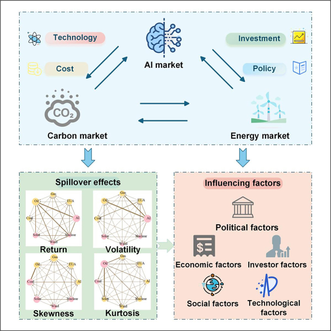 Figure 1
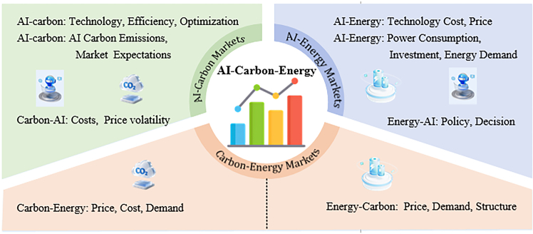 Figure 2
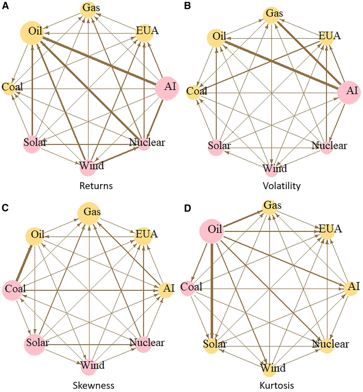 Figure 3
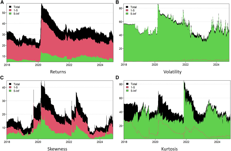 Figure 4
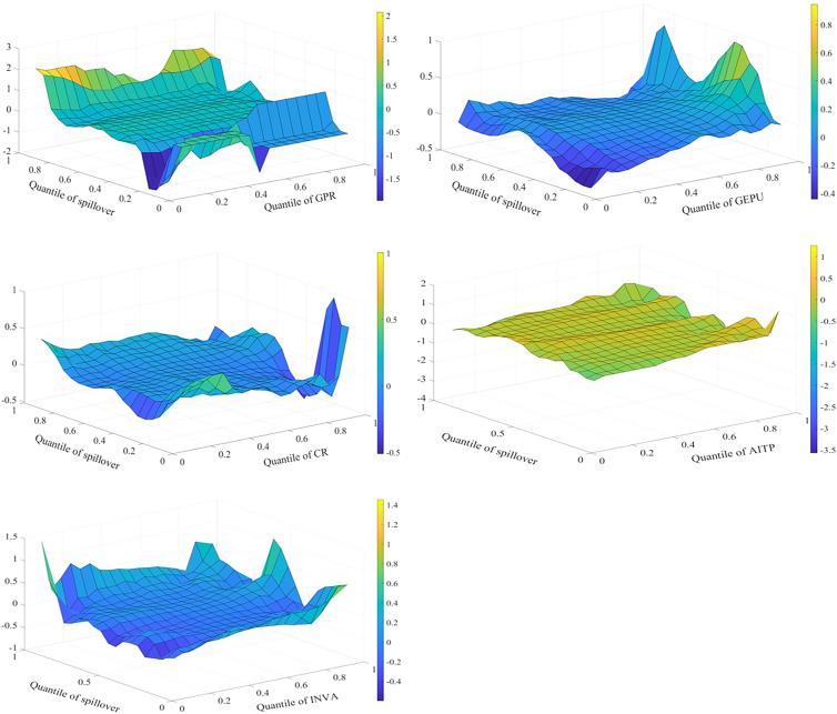 Figure 5
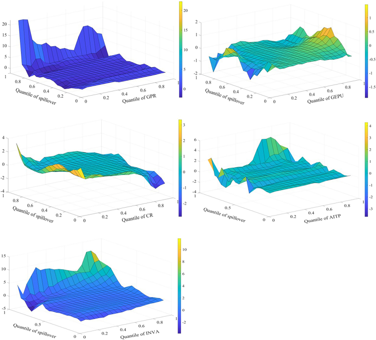 Figure 6
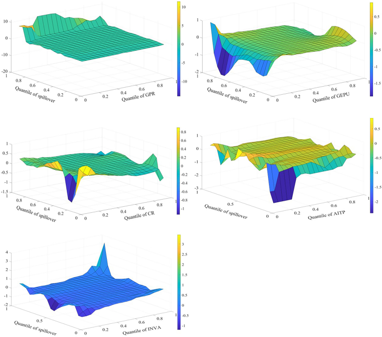 Figure 7
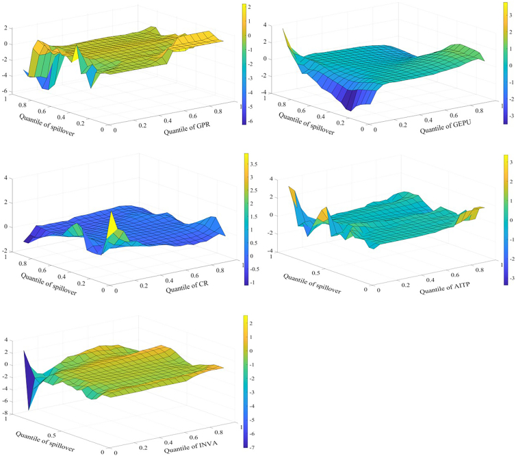 Figure 8
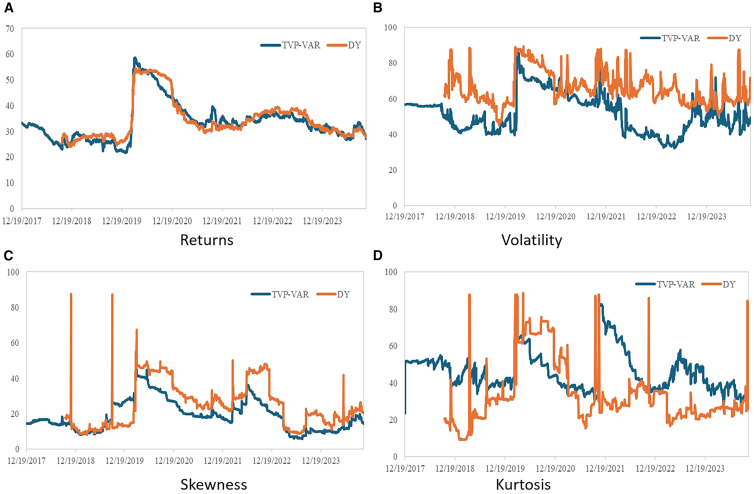 Figure 9
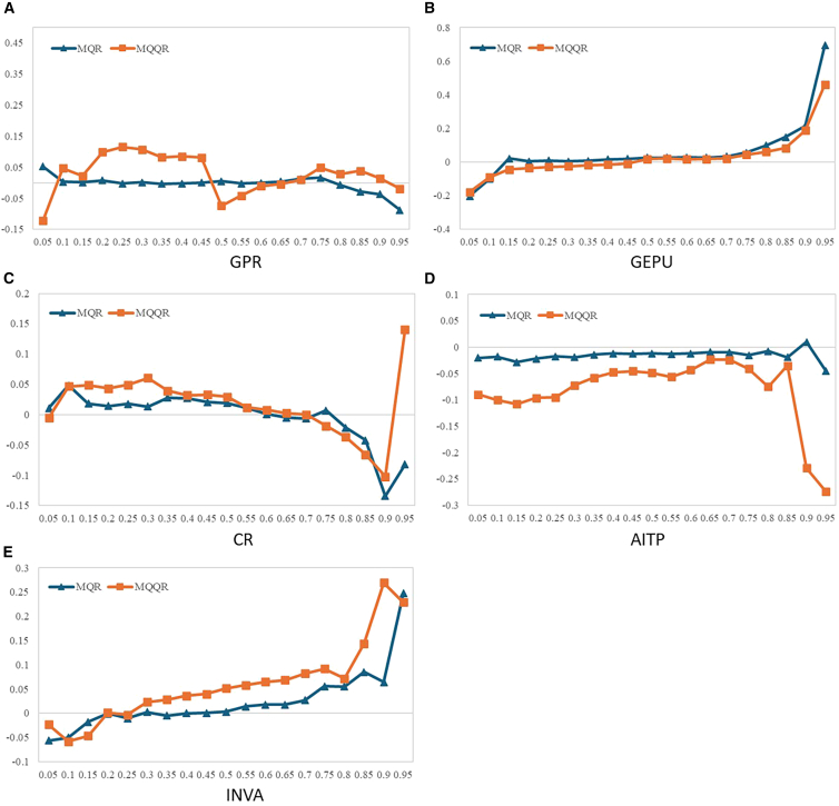 Figure 10
Peer Reviews
No public reviews on file for this paper yet. If you reviewed it on a platform where reviews are public (OpenReview, ICLR, NeurIPS, ICML), you can paste yours below so the community can read it here.
Videos
No videos yet. Explain this paper in a talk, walkthrough, or lecture? Add one.
Taxonomy
TopicsMarket Dynamics and Volatility · Energy, Environment, Economic Growth · Global Energy Security and Policy
Introduction
Artificial intelligence (AI) is broadly defined as an intelligent system capable of thinking and learning; the system includes tools, technologies, and algorithms that emulate human cognition and behavior patterns.1^,^2 AI has become a key driving force for technological innovation and industrial upgrading.2 AI is increasingly being integrated with energy-saving and decarbonization technologies across sectors, constructing many “AI+” industrial ecosystems. The link between the AI market and the carbon market is gradually strengthening. For example, the rapid development of AI technology, such as advances in machine learning, big data analytics, and predictive modeling, provides new tools to optimize carbon markets and forecast carbon emissions.3^,^4^,^5 In the development of nowadays carbon markets, AI enables in-depth analysis of trading data and policy dynamics through functions such as constructing intelligent carbon quota allocation algorithms, developing transaction risk early-warning models, and implementing dynamic assessments of emission reduction outcomes. This facilitates precise trading decision support and promotes the efficient operation of carbon markets.6 By 2050, the adoption of AI technologies is expected to reduce energy consumption and carbon emissions by approximately 8%–19%.7
Further, AI and energy markets have formed a “symbiotic relationship.” Energy is a foundational fuel for AI advancement, while AI drives cost reductions in energy consumption, increases efficiency, and optimizes resource allocation across energy systems.8^,^9 This illustrates the deep internal link among the AI, carbon, and energy markets. It is reported that 56% of global energy companies are expanding the scale of their AI projects, while 44% have integrated AI into core operational processes. AI has evolved from an optional technology to a mandatory strategic option. For instance, in the hydropower sector, China Huadian Corporation developed the world’s first large-scale runoff prediction model. Through AI algorithm optimization, it has increased hydropower utilization rates from an average of 5.8% annually over the past decade to 10.8%, demonstrating how AI significantly enhances energy efficiency.
Given the increasingly strong connections between the AI, carbon, and energy markets, the spillover effects among the three markets cannot be overlooked. Figure 1 illustrates the spillover pathways among the three markets. The risk spillover from the AI market to the carbon market primarily occurs through two pathways. First, AI can enhance production efficiency and optimize industrial structures, thereby reducing corporate costs and carbon emissions, which in turn influences carbon prices.10^,^11 Second, AI generates substantial carbon emissions. Combined with environmental pressures, this creates market expectations that the AI sector will purchase more carbon allowances, thereby influencing carbon prices.12^,^13 The spillover effects from the carbon market to the AI market can be analyzed from the perspective of corporate costs. Fluctuations in carbon prices affect the operating costs of AI enterprises, leading to stock price volatility in the AI market.Figure 1. Framework of spillover effect pathways
The spillover effects from the AI market to the energy market primarily manifest through two pathways, including cost pathway and investment pathway. First, AI-driven technological advances reduce the cost of new energy technologies, enhance core competitiveness, and influence energy prices. Second, the substantial energy consumption of AI computing power, compounded by environmental pressures, drives AI corporations to invest in renewable energy, thereby affecting energy demand. Then, the spillover effects from the energy market to the AI market can be analyzed from a policy perspective. For instance, when governments implement new energy subsidy policies, it may change AI corporations’ investment decisions and impact the AI market.14
Spillover effects also exist between carbon markets and energy markets. Carbon prices influence energy demand by affecting corporate carbon emission costs, thereby impacting energy prices.15^,^16^,^17 Fluctuations in energy prices affect production costs and fuel choices at the corporate level, subsequently influencing carbon emission levels and carbon allowance prices.18^,^19^,^20 The European Union carbon futures market is a good illustration, as it has experienced three major turbulence cycles: the 2008 financial crisis, the sovereign debt crisis, and the post-pandemic energy trilemma (COVID-19, economic rebound, and supply shocks).21^,^22 The volatility was contagious and was amplified by growing market symbiosis.
Previous studies have yielded significant theoretical and empirical findings regarding the spillover effects in markets and their influencing factors. However, there are several critical research gaps to address. AI is increasingly becoming a core technological support for carbon markets and energy markets, playing a pivotal role in carbon emission monitoring and optimizing energy structures. While the interconnection between AI and these markets continue to intensify, little scholarly attention has focused on tri-market spillover effects. Previous studies on risk transmission mechanisms predominantly rely on first- and second-order moments of asset return distributions23^,^24; these do not fully capture financial risks during extreme market conditions and do not consider higher-order moment risks. Further, previous analyses of spillover determinants tend to examine specific factors or limited combinations and have not applied a comprehensive multi-factor approach. Methodologically, studies generally focus on average effects or examine spillover quantiles in isolation, without a concurrent analysis of market spillover effects and their determinants across different quantile conditions.
This study measures the spillover effect among the AI markets, the international carbon market, the traditional energy market, and the new energy market. The research also explores the factors influencing the spillover effect. First, based on the returns, the Glosten-Jagannathan-Runkle generalized autoregressive conditional heteroskedasticity with skewness and kurtosis (GJRSK) model is used to calculate conditional volatility, skewness, and kurtosis. This introduces higher-order moments to measure asymmetric and tail risks in the markets. Second, a time-varying parameter vector autoregression (TVP-VAR) model is used to analyze static spillover effects, spillover networks, and dynamic spillover changes among carbon, energy, and AI markets. Finally, a multivariate quantile-on-quantile regression (MQQR) model reveals the influence of macro and micro factors on the spillover effects among multiple markets under different quantiles.
This is the first known study to simultaneously focus on the spillover effects among the AI, carbon, and energy markets. In doing so, it makes two key contributions in this field. First, it integrates AI market into the risk spillover analysis framework of carbon and energy markets. This facilitates the revelation of the networked characteristics of risk transmission among the three major systems, digital technology, energy transition, and environmental regulation, thereby providing the micro-foundation for constructing a complex risk theory in the “digital-green” era. It pioneers the analysis of higher-order connectedness (including asymmetric and tail risks) beyond traditional first/second moment approaches. This provides new insights into extreme market conditions that conventional spillover studies have not considered. Second, the study develops a comprehensive macro-micro analysis framework using MQQR modeling that simultaneously examines multiple influencing factors across different quantiles. This mitigates the limitations of previous studies that focus only on single macro-factors or average effects. These innovations deepen descriptions of dynamic market linkages and provide practical tools for investors and policymakers to better manage cross-market risk transmission and increase financial stability.
The risk spillover between carbon, energy, and AI markets
Table 1 summarizes previous studies about spillover effects among the carbon, energy, and AI markets. These studies are classified based on five attributes: markets, dimensions, region/countries, periods, and methods.Table 1. Summary of studies on spillover effects between the three marketsStudyMarketsDimensionCountryPeriodsMethodsTiwari et al.25Carbon and AI marketsReturnsWorldwide2017–2020Time-varying Markov switching copula modelSong et al.26Carbon and fossil energy marketsVolatilityChina2014–2021VAR, BEKK-MGARCHLovcha et al.27Carbon, fossil energy, and electricity marketsReturnsEurope2008–2018SVARQiao et al.28Carbon, fossil energy, and electricity marketsReturnsWorldwide2009–2022TVP-VAR-SVSu et al.23Carbon and energy marketsReturns, volatilityEurope2018–2022QVARYe et al.29Carbon, fossil energy, and electricity marketsReturnsWorldwide2017–2023QVARWu and Qin30Carbon and new energy marketsVolatilityChina2014–2022DCC-GARCHJiang et al.24Carbon and energy marketsVolatilityWorldwide2019–2023QVARChu et al.31Carbon and fossil energy marketsSkewness, kurtosisWorldwide2012–2022QVARXu et al.32Carbon and AI marketsReturnsChina2022–2023TVP-VARYousaf et al.33Fossil energy, AI tools, and marketsVolatilityWorldwide2019–2023QVARGhaemi Asl et al.34Clean energy and AI marketsReturnsWorldwide2018–2023TVP-VARLiu et al.35Energy and AI marketsReturnsWorldwide2017–2023Quantile regressionZeng et al.36Clean energy and AI marketsVolatilityWorldwide2017–2023QVAR, WLMCGubareva et al.19Fossil energy, clean technology, and AI marketsReturnsWorldwide2018–2023Generalized quantile-on-quantile regressionLiu et al.37Carbon and fossil energy marketsReturnsChina2021–2022TVP-VARXu et al.38Carbon and energy marketsReturnsWorldwide2012–2023TVP-VAR-BKManeejuk et al.39Carbon and energy marketsVolatilityWorldwide2014–2023Copula quantile regressionQVAR, Quantile Vector Auto-Regression; SVAR, Structural Vector Auto-Regression; TVP-VAR, Time-Varying Parameter Vector Auto-Regression; TVP-VAR-SV, Time-Varying Parameter Vector Auto-Regression with Stochastic Volatility; TVP-VAR-BK, Time-Varying Parameter Vector Auto-Regression with Bekaert-Harvey; BEKK-MGARCH, Bollerslev-Engle-Kraft-Kroner Multivariate Generalized Autoregressive Conditional Heteroskedasticity; DCC-GARCH, Dynamic Conditional Correlation Generalized Autoregressive Conditional Heteroskedasticity; WLMC, Wavelet Local Multiple Correlations.
Early studies on this topic focused on the spillover effects between energy markets and carbon markets.23^,^24^,^26^,^27^,^28^,^29^,^30^,^31^,^37^,^38^,^39^,^40 As the AI market has grown, however, its interaction with carbon markets has continued to attract more attention.25^,^32 Previous research found that AI can significantly affect carbon emissions. The combination of AI technology with energy-saving and carbon-reducing technologies can achieve energy-saving and carbon-reducing effects.7^,^41^,^42^,^43^,^44
In addition, scholars have begun to explore the connection between the AI market and energy market.19^,^33^,^34^,^35^,^36 AI provides advanced data analytics capabilities and machine learning algorithms and is now widely used to predict energy production, demand, and power generation.8^,^45^,^46 However, as AI-related technologies continue to develop, and AI links with the carbon and energy markets gradually strengthen, more research is needed about the spillover effects among the three markets.
In terms of the spillover dimension, most studies have focused on first- and second-moment spillover effects. First- and second-moment spillovers represent traditional and fundamental risk transmission mechanisms, referring to return and volatility spillovers, respectively. These focus on price direction and volatility magnitude. Higher-order moment spillovers represent deeper and more disruptive risk transmission. Third- and fourth-moment spillovers correspond to skewness and kurtosis spillovers, respectively, focusing on the asymmetry and heavy-tailed peaks of the return distribution. Most studies on risk transmission effects primarily focus on return and volatility spillover effects. This does not represent the financial risk under extreme market conditions and highlights the need for more research on the risks associated with higher-order moments. In terms of study area, most research has focused on the worldwide market. The research methods used in previous studies include vector auto-regression, quantile vector auto-regression, structural vector auto-regression, and Generalized Autoregressive Conditional Heteroskedasticity (GARCH) methods. These models, however, have problems with respect to overly subjective window selection and do not reflect dynamic changes in spillover effects.
In contrast, the TVP-VAR model provides a new time-varying perspective on spillover effects and does not require the independent setting of rolling window sizes. This means it avoids the problems of subjective window size settings and data loss. Given this benefit, this study simultaneously explores the spillover effects of the three markets (AI, carbon, energy) using the TVP-VAR model and explores the changes in spillover effects under extreme risks using the higher-order moments perspective.
The factors influencing spillovers in carbon, energy, and AI markets
Understanding spillover effects among the three markets of interest is an important first step. The next step is describing the factors influencing those spillover effects, to help investors and policymakers with portfolio management and risk management. Some studies have explored the factors influencing spillovers. These studies are summarized in Table 2 and are classified based on six attributes: markets, influencing factors, periods, methods, and whether the study considers the quartile of spillovers and the quartile of influencing factors.Table 2. Studies on factors that influence spillover effectsStudyInfluencing factorsMarketsPeriodsMethodsQuantile of spillovers?Quantile of influencing factors ?Tan et al.47Economic policy uncertaintyCarbon, energy, and finance markets2008–2018Multivariate linear regression––Xiao and Wang48Investor attentionOil market2004–2020Linear regression––Tiwari et al.25Economic policy uncertaintyCarbon and AI markets2017–2020Multivariate linear regression––Ma et al.49Economic policy uncertaintyElectricity markets2009–2020Multivariate linear regression––Ding et al.50Investor attentionCarbon and energy markets2010–2021Nonparametric causality-in-quantiles test✓–Zhou et al.16Climate riskCarbon, energy, and metals markets2015–2022Quantile-on-quantile regression✓✓Chen et al.51Climate riskCarbon and stock markets2014–2022Comparing different time periods––Wu and Liu52Investor attention and climate policy uncertaintyGreen finance markets2014–2022GARCH-MIDAS––Man et al.53Investor attention and economic policy uncertaintyCarbon, energy, and finance markets2014–2022Quantile granger causality test✓–Chen et al.54Climate riskFossil and clean energy markets2015–2022Comparing different time periods––Guo et al.55Climate riskEnergy markets2016–2023Quantile regression✓–Xing et al.56Climate riskClean energy and non-ferrous metals markets2018–2023GARCH-MIDAS––Dong et al.40Climate riskCarbon and energy markets2017–2022GJR-GARCH-MIDAS––Wang et al.57Geopolitical risksEnergy futures markets2018–2022Random forest––Li et al.58Geopolitical risksFinancial markets2021–2023Comparing different time periods––Huang et al.59Geopolitical risksEnergy and metal markets2011–2024Quantile regression✓–Liu et al.37Geopolitical risksCarbon and energy markets2021–2022Comparing different time periods––Zhang et al.60Geopolitical risksEnergy and financial markets2018–2022Comparing different time periods––GARCH-MIDAS, Generalized Autoregressive Conditional Heteroskedasticity with Mixed Data Sampling; GJR-GARCH-MIDAS, Glosten-Jagannathan-Runkle GARCH-MIDAS.
In terms of markets, previous studies mainly focused on the energy, carbon, and financial markets.37^,^47^,^55^,^58^,^60 Studies have not yet focused on the factors influencing the spillover between AI and other markets. In terms of other influencing factors, on the macro side, some studies report that the intensity of spillover effects is influenced by factors such as geopolitical changes, economic policy changes, and extreme climate.51^,^54^,^58^,^61 In addition, some studies have applied a micro perspective to explore the factors of spillovers.48^,^50^,^52^,^53 However, most studies exploring the factors influencing spillover effects focus on a single or two influencing factors; few studies comprehensively analyze multiple influencing factors. Therefore, this study comprehensively analyzes the impact of the following factors on spillover effects from macro and micro perspectives: geopolitical risk (GPR); economic policy uncertainty (EPU); climate risk (CR); AI technological progress (measuring using patents [AITP]); and investor attention to AI, carbon, and energy markets (measured using the Google Search Volume Index [INVA]). At the macro level, GPR represents political factors, EPU represents economic factors, CR represents social factors, and AITP represents technological factors. At the micro level, INVA represents investor concerns.
In terms of methods, previous studies have mainly used a multivariate linear regression model, GARCH with mixed data sampling model, and quantile regression model. These methods only analyze average impacts or consider different quantiles of the spillover effect; this approach does not analyze both the market spillover effect and the influencing factors when in different quantiles. Therefore, this study adopts the MQQR model and considers situations where the independent and dependent variables are at different quantiles.
In conclusion, it is evident that previous studies have yielded significant findings regarding the spillover effects in markets and their influencing factors. However, several research issues remain to be further explored. First, existing studies lack discussion on spillover effects among the AI, carbon, and energy markets. It is essential to consider spillover effects among the three markets for risk prevention and investment decision-making. Second, there are insufficient analyses of spillover effects from extreme risks. When quantifying cross-market spillover effects, skewness and kurtosis spillovers should also be considered. Third, researches on the factors influencing spillover effects remains insufficient. Considering multiple factors influencing spillover comprehensively and analyzing scenarios across different quantiles would enhance the effectiveness of preventing inter-market risks.
Results
Static spillover effects
The data sources of markets and influencing factors are summarized in Tables 3 and 4. Table 5 shows the parameters estimated by the GJRSK model. Table 6 provides the descriptive statistics. Most of the markets show positive average returns during the sample period; European Union allowance futures (EUA) has the highest returns. The maximum and minimum values represent the gains and losses, respectively. The maximum losses of the market all exceed the maximum gains in absolute terms. Skewness and kurtosis statistics demonstrate non-normal return and volatility series distributions. Most variables show negative skewness over the sample period, indicating that most market return distributions are left-skewed; the exception is natural gas. The kurtosis values of all market return distributions exceed 3, indicating that the data distributions are sharper than the normal distribution with higher peaks and wider tails. This result is further supported by the Jarque-Bera statistics, indicating that the null hypothesis of normality is rejected in all series.Table 3. Data for three marketsMarketIndexAbbreviationData sourceCarbon marketEuropean Union allowance futuresEUAIntercontinental ExchangeTraditional marketsCoal marketRotterdam coal futuresCoalIntercontinental ExchangeOil marketBrent crude oil futuresOilIntercontinental ExchangeNatural gas marketPort Henry natural gas futuresGasEnergy Information AdministrationNew energy marketsSolar marketNASDAQ OMX Solar IndexSolarNASDAQ websiteWind marketNASDAQ OMX Wind IndexWindNASDAQ websiteNuclear marketMVIS Global Uranium and Nuclear IndexNuclearMarketVector websiteAI marketNASDAQ Global CTA Artificial Intelligence and Robotics IndexAINASDAQ websiteTable 4Data for influencing factorsInfluencing factorsIndexAbbreviationData sourcePolitical factorsGeopolitical risk indexGPRCaldara and Iacoviello (2022)Economic factorsGlobal economic policy uncertainty indexGEPUBaker et al. (2016)Social factorsGlobal frequency of climate-related disastersCREmergency Events DatabaseTechnological factorsAI patentsAITPWorld Intellectual Property OrganizationInvestor factorsInvestor attention indexINVAGoogle TrendsTable 5Parameters estimated by GJRSK modelParameterAIEUAGasOilCoalSolarWindNuclearMean equationα_1_0.158∗∗∗−0.040∗∗−0.0220.069∗∗∗0.096∗∗∗0.106∗∗∗0.078∗∗∗0.001Variance equationβ_0_0.056∗∗∗0.363∗∗∗0.034∗∗0.182∗∗∗0.075∗∗∗0.110∗∗∗0.046∗∗∗0.033∗β_1_0.036∗0.055∗∗∗0.039∗∗0.0270.0250.039∗∗0.056∗∗∗0.045∗∗β_2_0.062∗∗∗0.0180.0040.099∗∗∗0.0010.040∗∗0.053∗∗∗0.035∗β_3_0.896∗∗∗0.8780.956∗∗∗0.874∗∗∗0.969∗∗∗0.914∗∗∗0.877∗∗∗0.900∗∗∗Skewness equationγ0−0.147∗∗∗−0.041∗∗0.059∗∗∗−0.211∗∗∗−0.042∗∗0.059∗∗∗−0.048∗∗∗−0.047∗∗γ_1_0.0290.0120.0190.192∗∗∗0.147∗∗∗0.0040.006−0.088∗∗∗γ2−0.050∗∗∗−0.0020.021−0.188∗∗∗−0.149∗∗∗0.052∗∗∗0.088∗∗∗0.196∗∗∗γ_3_0.186∗∗∗0.0070.363∗∗∗0.175∗∗∗−0.0020.218∗∗∗−0.102∗∗∗−0.109∗∗∗Kurtosis equationδ_0_1.492∗∗∗2.928∗∗∗1.432∗∗∗1.803∗∗∗3.504∗∗∗1.653∗∗∗2.616∗∗∗3.258∗∗∗δ_1_0.0070.0090.0000.0000.0000.0000.0070.000δ_2_0.049∗∗∗0.0130.0230.0000.0000.0150.0000.053∗∗∗δ_3_0.521∗∗∗0.125∗∗∗0.581∗∗∗0.460∗∗∗0.239∗∗∗0.503∗∗∗0.220∗∗∗0.000^∗∗∗^, ^∗∗^, and ^∗^ denote 1%, 5%, and 10% level of significance, respectively.Table 6. Descriptive statisticsMinMaxMeanMedianSkewnessKurtosisStd. DevJ-BADFLjung-Box (10)ARCH-LM (10)NAI−10.489.100.020.09−0.495.731.382507.50∗∗∗−11.21∗∗∗894.12∗∗∗361.45∗∗∗1772EUA−17.7316.140.120.10−0.464.402.741496.20∗∗∗−12.45∗∗∗198.83∗∗∗114.90∗∗∗1772Gas−21.3321.030.000.000.044.393.881425.90∗∗∗−11.01∗∗∗99.66∗∗∗80.97∗∗∗1772Oil−26.0013.520.010.19−1.4316.212.4120057.00∗∗∗−12.21∗∗∗247.18∗∗∗151.53∗∗∗1772Coal−53.6932.620.010.00−2.5466.493.17329075.00∗∗∗−11.93∗∗∗63.47∗∗∗51.48∗∗∗1772Solar−14.9611.320.03−0.02−0.173.812.251086.10∗∗∗−11.14∗∗∗480.01∗∗∗246.79∗∗∗1772Wind−12.599.890.020.05−0.5811.261.229493.80∗∗∗−11.39∗∗∗912.18∗∗∗388.06∗∗∗1772Nuclear−10.857.350.030.06−0.8412.491.1311761.00∗∗∗−12.44∗∗∗1414.00∗∗∗552.64∗∗∗1772J-B, Jarque-Bera test; ADF, Augmented Dickey-Fuller test; ARCH-LM, Autoregressive Conditional Heteroskedasticity-Lagrange Multiplier test.^∗∗∗^, ^∗∗^, and ^∗^ denote 1%, 5%, and 10% level of significance, respectively.
In addition, the study performs a unit root test using the Augmented Dickey-Fuller test. The result shows that all the variables are smooth at 1% level of significance. The autoregressive conditional heteroskedasticity-Lagrange multiplier test confirms the presence of an autoregressive conditional heteroskedasticity effect in this time series. Therefore, the series characteristics make it appropriate to use the GJRSK model and the spillover analysis model.
This study uses the TVP-VAR model to analyze the static spillover effects of the carbon, energy, and AI markets. The frequency domain has two types of timescales, including high frequency (1–5 trading days) and low frequency (>5 trading days). This enables a comprehensive understanding of the entire transmission chain from “short-term information shocks” to “long-term risks” through a multi-timescale perspective. High-frequency spillovers primarily capture instantaneous linkages driven by short-term market sentiment and breaking news events. It reflects the market’s rapid reaction and digestion of immediate information, exhibiting high volatility but weak persistence. Low-frequency spillovers mainly capture long-term shocks driven by macroeconomic trends and structural policy adjustments, characterized by slow changes but stable trends. Tables 7, 8, 9, and 10 show the results of static spillovers between the carbon, energy, and AI markets. “TO” represents the value of the spillover transmitted to other markets, and “FROM” represents the value of spillovers received from other markets. “NET” represents the net spillover. A positive net spillover value indicates that the market is a net transmitter of risk, and a negative net spillover value indicates that the market is a net receiver of risk. “TCI” represents the total spillover and measures the overall extent of information transfer and spillover among markets.Table 7. Return spillover resultsAIEUAGasOilCoalSolarWindNuclearFROMPanel A: Total spilloverAI45.881.590.522.820.3719.7816.8312.254.12EUA2.7281.871.423.163.551.952.372.9518.13Gas1.11.6790.221.41.461.40.941.799.78Oil4.833.251.4275.751.823.93.65.4324.25Coal0.823.161.352.0291.160.450.410.628.84Solar20.151.330.842.420.2947.8818.478.6352.12Wind17.451.510.592.290.3418.7144.5414.5755.46Nuclear13.681.870.953.490.259.5515.9754.2445.76TO60.7614.377.0917.618.0855.7558.646.19TCINET6.64−3.76−2.69−6.64−0.773.643.140.4438.35Panel B: High frequency (1 day to 5 days)AI34.891.230.372.230.2514.5912.669.1640.5EUA2.167.731.192.643.11.551.942.4314.95Gas0.921.4175.481.211.111.130.771.387.93Oil3.592.65160.921.32.892.833.9518.21Coal0.542.531.081.4471.180.320.290.426.62Solar15.360.960.571.830.2436.5213.796.439.15Wind12.261.10.451.750.2512.8633.6310.2438.91Nuclear10.411.450.682.840.187.1412.5241.5835.21TO45.1811.335.3413.946.4340.4844.7933.99TCINET4.68−3.62−2.59−4.28−0.191.345.88−1.2228.78Panel C: Low frequency (5 days to infinity)AI10.980.360.160.590.125.194.173.0413.62EUA0.6214.140.230.520.450.40.430.523.18Gas0.190.2614.740.190.350.270.180.411.85Oil1.240.60.4214.830.511.010.771.486.04Coal0.280.630.270.5819.980.130.120.22.22Solar4.790.360.260.590.0511.364.682.2312.97Wind5.190.410.140.540.095.8510.94.3416.55Nuclear3.280.420.260.650.072.423.4512.6710.55TO15.583.041.753.681.6415.2713.8112.21TCINET1.96−0.14−0.1−2.36−0.572.3−2.741.669.57Table 8Volatility spillover resultsAIEUAGasOilCoalSolarWindNuclearFROMPanel A: Total spilloverAI40.244.382.925.152.8716.4414.7213.2859.76EUA9.6460.393.343.242.626.137.287.3639.61Gas10.574.861.225.45.85.52.893.8238.78Oil14.695.942.7348.282.4410.516.58.9251.72Coal4.686.476.082.5166.735.984.073.4733.27Solar15.144.162.736.043.5738.6518.2611.4661.35Wind15.423.883.496.113.3316.8233.9417.0266.06Nuclear17.613.323.265.774.7212.8815.137.3562.65TO87.7532.9424.5434.2225.3674.2568.8265.33TCINET27.99−6.67−14.24−17.5−7.9112.92.762.6759.03Panel B: High frequency (1 day to 5 days)AI2.590.090.090.10.110.610.470.481.94EUA0.225.140.230.220.150.190.220.211.44Gas0.20.071.850.050.110.080.090.120.72Oil0.350.320.185.80.090.310.280.381.9Coal0.070.080.110.052.020.050.080.070.51Solar0.730.180.10.150.052.650.630.372.24Wind0.720.130.190.210.090.913.350.93.13Nuclear0.50.090.090.190.090.320.622.761.9TO2.790.950.990.980.692.452.392.54TCINET0.86−0.490.27−0.930.190.22−0.750.641.97Panel C: Low frequency (5 days to infinity)AI37.664.292.835.062.7615.8414.2612.857.82EUA9.4255.253.113.022.475.947.067.1438.17Gas10.374.7459.375.355.695.422.793.738.06Oil14.335.622.5542.472.3610.26.228.5449.82Coal4.616.395.972.4664.725.933.993.432.76Solar14.413.972.625.893.513617.6311.0959.11Wind14.713.753.35.93.2415.9130.5916.1262.93Nuclear17.113.233.175.584.6312.5614.4834.5960.75TO84.9531.9923.5533.2524.6671.866.4362.79TCINET27.13−6.18−14.51−16.58−8.112.693.52.0457.06Table 9Skewness spillover resultsAIEUAGasOilCoalSolarWindNuclearFROMPanel A: Total spilloverAI74.851.290.530.981.718.866.265.525.15EUA2.0486.172.90.911.822.261.622.2713.83Gas1.882.8686.550.851.152.521.692.513.45Oil0.71.810.689.795.010.60.461.0110.21Coal0.390.910.992.0392.930.410.641.697.07Solar7.722.121.150.860.5171.9211.024.6828.08Wind5.420.660.930.770.412.2170.928.6929.08Nuclear4.940.910.910.410.826.149.876.0723.93TO23.0910.578.026.8311.4333.0231.526.34TCINET−2.06−3.26−5.43−3.384.364.942.422.4121.54Panel B: High frequency (1 day to 5 days)AI55.420.990.370.61.35.193.643.4115.52EUA1.5466.982.340.691.261.540.991.599.95Gas1.231.5957.290.50.661.621.021.688.29Oil0.380.930.2964.661.950.370.330.574.83Coal0.20.520.691.3768.420.230.430.553.99Solar5.331.490.720.510.2750.127.293.0318.64Wind4.120.540.670.590.268.6658.896.8621.69Nuclear3.650.760.670.280.424.126.7862.1216.68TO16.466.825.734.556.1221.7220.4717.7TCINET0.94−3.12−2.56−0.282.133.08−1.221.0314.23Panel C: Low frequency (5 days to infinity)AI19.430.30.170.380.413.672.622.099.64EUA0.519.190.570.220.570.720.630.683.88Gas0.651.2729.260.350.490.910.670.825.16Oil0.320.880.3225.133.060.240.130.445.38Coal0.190.390.30.6724.510.180.211.143.08Solar2.390.640.440.350.2421.83.741.659.44Wind1.30.120.260.180.143.5612.031.837.39Nuclear1.290.150.240.130.42.023.0213.957.25TO6.633.752.292.285.3111.311.038.64TCINET−3−0.13−2.88−3.12.231.863.641.397.32Table 10Kurtosis spillover resultsAIEUAGasOilCoalSolarWindNuclearFROMPanel A: Total spilloverAI50.7911.9915.477.978.498.585.7149.21EUA2.4865.182.6714.117.812.582.232.9334.82Gas3.42.3461.7115.8410.431.91.932.4638.29Oil3.062.12.6454.9327.982.274.742.2745.07Coal2.5122.6737.948.850.893.172.0251.15Solar9.771.032.4223.348.9742.936.774.7857.07Wind7.570.671.3316.699.245.453.665.4546.34Nuclear5.781.11.9213.166.287.518.2256.0243.98TO34.5710.2415.63136.578.6829.0435.6325.62TCINET−14.64−24.58−22.6691.4327.53−28.02−10.71−18.3552.27**Panel B: High frequency (1 day to 5 days)AI25.270.20.361.020.573.912.982.0411.07EUA1.3548.251.663.331.781.130.981.9912.22Gas0.810.7127.031.711.140.730.380.656.13Oil0.720.340.3511.744.531.081.360.458.82Coal0.570.250.584.7215.410.20.740.247.31Solar4.180.250.563.010.8322.022.521.7913.14Wind4.290.180.343.031.722.94352.9315.43Nuclear3.450.670.93.881.964.884.1542.9419.9TO15.372.594.7520.7112.5414.8613.1210.08TCINET4.3−9.62−1.3811.885.231.72−2.31−9.8213.43Panel C: Low frequency (5 days to infinity)**AI25.530.81.6214.457.44.585.613.6838.13EUA1.1416.941.0110.776.031.451.240.9522.6Gas2.591.6334.6714.139.291.171.541.8232.17Oil2.351.762.2943.1923.441.23.381.8336.24Coal1.941.742.0833.1833.440.682.431.7843.84Solar5.580.781.8620.338.1320.914.252.9843.93Wind3.280.490.9913.657.522.4618.662.5230.91Nuclear2.330.431.029.284.332.634.0613.0824.08TO19.27.6410.88115.7966.1414.1822.5115.54TCINET−18.93−14.96−21.2879.5522.3−29.74−8.4−8.5338.84
Table 7 shows the spillover effects for returns. The total return spillover effect is 38.35%. This means that, on average, 38.35% of the price movements in each market are due to price movements in other markets. The AI market (60.76%) and the wind market (58.6%) have the strongest spillover effect (TO). This highlights the dominant role of the AI and wind markets in risk transmitting. This may be because rapid growth in the AI and wind energy markets is accompanied by technological uncertainty; the associated risks can quickly spread to other markets. These are also large receiving markets (FROM), indicating that markets with high-risk spillovers are also susceptible to shocks in other markets. At high and low frequencies, the total return spillover values are 28.78% and 9.57%, respectively. The connectedness decreases as the frequency bands increase. This indicates that the return spillover effects between these markets are more affected by short-term effects. The AI market is the largest spillover market in both the short and long term, and the solar and wind markets are the largest receiving markets.
Table 8 shows the results of the volatility spillovers. The total volatility spillover is 59.03%. This indicates that, on average, 59.03% of the market volatility is due to the volatility of the other markets. This demonstrates the strong volatility spillover effect among the three markets. AI is the largest-risk spillover market (87.75%), and wind energy is the largest-risk receiving market (66.06%) for the volatility spillover. This result aligns with the results for return spillovers. Meanwhile, the oil market is a net risk receiver in both the return and volatility spillovers. This is mainly because oil plays a crucial role in the global energy supply and is highly influenced by other markets. The total systematic spillover values at high and low frequencies are 1.97% and 57.06%, respectively. In both the short and long run, the AI market is the largest-risk spillover market, and the wind energy market is the largest-risk receiving market.
Table 9 shows the results of skewness spillovers. The total skewness spillover effect is 21.54%. This indicates that 21.54% of the asymmetry in the distribution of asset returns across markets is caused by other markets. In this case, the solar market is the largest-risk spillover market for the skewness spillover (33.02%) and the wind market is the largest-risk receiving market for the skewness spillover (29.08%). The total skewness spillover values at high and low frequencies are 14.23% and 7.32%, respectively. This indicates that short-term effects have a larger influence on the skewness spillover effect between these markets. Meanwhile, risk spillovers in the markets are heterogeneous across frequency bands. The risk transmitters and receivers in the markets vary with frequency bands.40 Specifically, the AI market is a net risk transmitter in the short term and shifts to being a net risk receiver in the long term. This may be because, in the short term, the high initial investment and technological uncertainty associated with AI lead to risks being easily transmitted to other markets. In the long term, however, the AI technology matures, and its specific applications depend on the carbon and energy markets. As such, the AI market may receive more risk transfers.
Table 10 shows the results associated with kurtosis spillovers. The total skewness spillover effect is 52.27%. This indicates that 52.27% of the probability of extreme returns occurring in each market is caused by other markets. This shows a strong kurtosis spillover effect among the three markets. The crude oil market is the largest-risk spillover market (136.5%), and the solar market is the largest-risk receiving market for the kurtosis spillover (57.07%). The risk spillover effect of the crude oil market is significantly stronger in the higher-order moments. At high and low frequencies, the total system spillover values are 13.43% and 38.84%, respectively. This indicates that long-term effects have a greater influence on the kurtosis spillover effect between these markets. In the long term, the AI market shifts from a net risk transmitter to a receiver, consistent with the findings of skewness spillovers.
Network connectedness analysis
This section builds upon these static spillover effects to further explore the network connectedness between markets, thereby facilitating a more intuitive understanding of spillover effects across markets. Figure 2 shows the net pairwise directional connectedness of the markets. The color of each node in the graph represents the market’s role in the spillover effect: pink indicates the market is a net transmitter, and yellow indicates the market is a net receiver. The size of the node indicates the market’s net pairwise spillover value. The arrow represents the direction of the spillover. Specifically, an arrow pointing from market A to market B indicates that market A transmits risk to market B. The thickness of the lines in the network diagram indicates the intensity of spillovers between markets; thicker line segments indicate stronger linkages between the two markets.Figure 2. Net-pairwise directional connectedness(A) Return spillover effect, (B) Volatility spillover effect, (C) Skewness spillover effect, (D) Kurtosis spillover effect.
Figure 2A shows that the AI market is the main transmitter in the return spillover network; the oil and carbon markets are the main receivers. This means the market price changes is mainly transmitted from the AI and new energy markets to the carbon and traditional energy markets. Figure 2B shows that the results of the volatility spillover network are similar to the results of the return connectedness network. This may be because AI and new energy have high investment demands and high uncertainty during development. As such, returns and volatility risks are quickly transmitted to other markets.
Figure 2C shows that, in the skewness spillover network, the AI market shifts from being a risk transmitter to being a risk receiver, and the coal market shifts to being a risk transmitter. Figure 2D shows that, in the kurtosis spillover network, all markets are risk receivers except for coal and oil markets. This indicates that the risk of extreme returns occurring is mainly transmitted from the coal and oil markets to other markets. The coal market is a net risk receiver in return spillovers and volatility spillovers. However, it transforms into a net risk transmitter in skewness and kurtosis spillovers. This indicates that the coal market rapidly propagates risk to other markets during extreme events. This highlights the need to monitor the skewness and kurtosis impacts of coal on other markets.
Dynamic spillover effects
Static spillover effects indicate the intensity and direction of markets but do not explain the dynamic process associated with the spillover. Figure 3 shows the dynamic spillover effects of returns, volatility, skewness, and kurtosis in the carbon, energy, and AI markets. The black shaded area represents the total spillover effect; the red and green shaded areas represent the short-term and the long-term spillover effects, respectively. A larger shaded area indicates there is a higher spillover effect among the markets.Figure 3. Dynamic overall spillovers(A) Return spillover effect, (B) Volatility spillover effect, (C) Skewness spillover effect, (D) Kurtosis spillover effect.
The results show that the spillover effects of all orders have significant time-varying characteristics. The spillovers of volatility and kurtosis are higher overall compared with those of returns and skewness, fluctuating between 20% and 85%. The red region dominates the return and skewness spillovers; the green region dominates the volatility and kurtosis spillovers. This indicates that return and skewness are dominated by short-term spillovers and volatility and kurtosis are dominated by long-term spillovers. These outcomes are consistent with the findings of the static spillovers.
In addition, there are multiple distinct peaks and periods of turbulence on the spillover curves. These may be because spillovers between markets are affected by external shocks, including unexpected events, economic events, and GPRs.61 For example, during the COVID-19 pandemic in 2020 and the outbreak of the Russia-Ukraine war in 2022, there was clear volatility in global markets, and the spillover effect reached a high level.
Brock-Dechert-Scheinkman nonlinearity test
This section analyzes the factors influencing spillover effects from macro and micro perspectives. Table 11 shows the descriptive statistics of the variables. The Augmented Dickey-Fuller test is tested for each variable, and all variables pass the smoothness test after first-order differencing. In addition, this study conducts the Brock-Dechert-Scheinkman (BDS) nonlinearity test.62 Table 12 shows the results. All variables are nonlinear over the study period. This affirms the applicability of the MQQR method for this study.Table 11. Descriptive statisticsNMeanStd. DevMedianMinMaxSkewnessKurtosisADFTCI117480.000.45−0.05−2.456.084.7247.26−8.61∗∗∗TCI217480.001.84−0.01−10.8430.533.6358.62−13.44∗∗∗TCI317480.001.010.00−5.7222.2112.11243.02−13.07∗∗∗TCI417480.011.870.10−10.8152.3614.94390.35−12.13∗∗∗GPR17484.680.464.702.256.29−0.260.95−5.89∗∗∗GEPU17485.490.225.464.836.07−0.050.04−3.62∗∗CR17483.810.253.833.044.500.090.96−8.30∗∗∗AITP17483.870.824.151.155.40−0.87−0.02−4.72∗∗∗INVA17483.070.472.941.544.300.19−0.52−5.95∗∗∗^∗∗∗^, ^∗∗^, and ^∗^ denote 1%, 5%, and 10% level of significance, respectively.Table 12. The results of the BDS testTCI1TCI2TCI3TCI4GPRGEPUCRAITPINVAI2.dim.z-sat9.09519.41114.94712.02428.766349.802250.961166.486163.500Prob0.000.000.000.000.000.000.000.000.003.dim.z-sat9.83125.15115.97713.49632.718690.693452.490270.638255.438Prob0.000.000.000.000.000.000.000.000.00
MQQR results and discussion
Spillover effects across markets are affected by multiple influencing factors that interact with one another. Therefore, this study employs the MQQR model to comprehensively examine the various factors affecting spillover effects. Figure 4 shows the effects of each factor on the spillover effect for returns. First, the situation where influencing factors are at different quantiles is analyzed. When GEPU and INVA are in the higher quantile (0.8–0.95), both have a significant positive impact on return spillovers. Economic policy is an important driver of credit flows and financial cycles; uncertainty increases the market’s sensitivity to negative information and affects investor expectations. Investors subsequently adjust their portfolios and change asset allocations. As a result, EPU affects supply and demand, increasing spillovers between markets. When investors pay more attention to the three markets of interest, market sentiment spreads quickly through channels such as social media. This can trigger a herd effect. As a result, investors increase the frequency of adjustments to assets. This increases the spillover effect among markets.Figure 4. Factors influencing returns spillover
When spillover effects are in different quantiles, the impact of influencing factors on the spillover effect also varies. AITP mainly reduces return spillovers. AI technology can improve market efficiency and reduce arbitrage opportunities through real-time data analytics, potentially reducing risk transmission between markets. Further, AI technology can help investors optimize their portfolios and better diversify risks, reducing market return spillovers. When return spillovers are in the high quantile (0.80–0.95), GPR, CR, and INVA all have a strong positive relationship with return spillovers. The effect of GPR is larger. GPR, CR, and other factors may work together in times of high market stress to affect energy supply and infrastructure across markets, exacerbating intermarket spillovers. During periods of high market uncertainty, investors may pay more attention to risk factors, leading to faster information transmission and more sensitive market reactions to negative information. This may increase return spillovers.
The effect of each factor on the volatility spillover effect is shown in Figure 5. Similar to the results for return spillovers, when GEPU and INVA are in the higher quantile (0.80–0.95), both have a significant positive impact on volatility spillovers. When the volatility spillover effect is in the high quantile (0.80–0.95), GPR and INVA are positively related to the effect. In addition, the results indicate that CR increases volatility spillovers when CR is in the low quantile and suppresses volatility spillovers when CR is in the high quantile. There are some possible reasons for this. During periods of low CR, short-term factors such as policy deregulation and technological breakthroughs may increase volatility spillovers between markets. When CR is high, markets are warned promptly of crisis events, such as extreme weather events. This allows investors to adjust their long-term positions and reduce their response to short-term volatility. Similar to the results of return spillover, when volatility spillovers are in the high quantile (0.80–0.95), GPR, CR, and INVA all have a strong positive relationship with volatility spillovers.Figure 5. Factors influencing volatility spillover
Figure 6 shows the effect of each factor on the skewness spillover effect. When GEPU is in the low quantile (0.05–0.25), it lowers the effect. When economic policies are more stable, investors have more consistent expectations about future policies, possibly leading to lower inter-market risk spillovers. Further, during periods of economic policy stability, there are fewer arbitrage opportunities, and investors may focus more on factors specific to their respective markets than on changes in macro policy. This may lower skewness spillovers. When CR is in the low quantile (0.05–0.25), it increases skewness spillovers. When the skewness spillover effect is in the higher quantile (0.80–0.95), GPR mainly increases the skewness spillover effect. This is consistent with the previous analysis.Figure 6. Factors influencing skewness spillover
Figure 7 shows the effects of the factors on kurtosis spillovers. When CR is in the lower quantile, it mainly contributes to these spillovers, consistent with the previous findings. When INVA is in the lower quantile, it slows down the kurtosis spillovers. The possible reasons are as follows. First, when investors are paying less attention, there is inefficient inter-market information transmission and a lack of common information or trading behavior among markets. Second, low investor attention may lead to reduced participation in the market. This lowers the transmission effect of volatility extremes between markets.Figure 7. Factors influencing kurtosis spillover
When kurtosis spillovers are in the high quantile (0.85–0.95), GPR and AITP can lower kurtosis spillovers. This result differs from the previous findings. This may be because when kurtosis spillovers are strong and GPR is elevated, investors may adopt hedging strategies and reduce their investments. This may lower the linkage of extreme events. In addition, advances in AI technology, such as predictive algorithms and risk modeling, increase the ability of markets to anticipate and respond to extreme events. This may reduce the linkage of extreme events.
It is found that there are several common conclusions. When GEPU and INVA are in the higher quantile (0.8–0.95), both have a significant positive impact on return and volatility spillover effects. Among the return, volatility, and skewness spillover effects, when the spillover effects are in the higher quantile range (0.8–0.95), GPR, CR, and INVA all exert a significant positive influence on the spillover effect. This indicates that GPR, GEPU, CR, and INVA primarily amplify spillover effects across markets. Among all spillover effects, AITP predominantly depresses spillover effects. This demonstrates that technological progress plays a significant role in mitigating risk spillovers between markets.
Robustness tests
To conduct the robustness tests, this study uses the connectedness model proposed by Diebold and Yilmaz (2012)63 and Diebold and Yılmaz (2014)64 in place of the TVP-VAR model. Table 13 shows that the results remain consistent for return, volatility, skewness, and kurtosis spillover indices among carbon, energy, and AI markets when using different estimation methods. The rolling window method is used to analyze the robustness of the dynamic spillover effect. Figure 8 shows that the trends with the two methods are consistent, indicating the results are robust. To assess the robustness of the influencing factors, this study applies the approach of Alola et al. (2023)65 and compares the results of the multivariate quantile regression model (MQR) with the results of the average of the MQQR. The results in Figure 9 show that the trends estimated by MQQR and MQR are approximately the same. This confirms the validity and robustness of the results.Table 13. Total spillover results (Diebold and Yilmaz model)AIEUAGasOilCoalSolarWindNuclearFROMPanel A: ReturnAI43.489061.1639640.2953252.5390810.1234319.7232318.0209114.6457.063868EUA2.32212486.043620.4873842.9395021.8974081.0071422.6167962.6860281.744548Gas0.6220040.49204894.962580.9856780.7752730.8175320.2300781.114810.629678Oil4.6558932.6300550.96481877.397611.2990123.6476723.7843535.6205862.825299Coal0.1137341.1029470.7226191.78903795.813420.1010720.1116830.2454910.523323Solar20.561950.5178440.5851612.1378650.04318446.0274720.13039.9962246.746567Wind18.373051.2845150.1941912.0873240.09359919.677541.9753616.314467.253079Nuclear16.497631.4918650.5810683.5273810.01740910.6640318.3237348.89696.387888TO7.8932981.0854050.4788212.0007330.5311646.9547727.9022316.32782533.17425Panel B: VolatilityAI29.715970.1734160.04190415.911930.42086517.5313217.8842618.320328.785503EUA15.1845842.18680.0400496.5519873.69290110.5016812.797959.0440557.22665Gas7.3380280.20510974.877540.2729046.3509971.942153.140515.8727593.140307Oil18.492150.7670820.33028841.993831.03950814.850659.55600312.970487.250771Coal0.1145157.4570425.0523070.50017783.381810.46772.5513050.475152.077274Solar21.056670.4121460.02492115.56570.10709527.8461619.380615.60679.019229Wind22.30990.3503720.10129416.950650.18573718.4456422.1327319.523689.733408Nuclear23.655970.6500980.07247616.44550.08651416.3587917.5764325.154219.355723TO13.518981.2519080.7079059.0248571.48545210.0122410.3608810.2266456.58887Panel C: SkewnessAI77.788380.0075950.0406030.0178060.26908910.145626.5297135.2011932.776452EUA0.24236392.695630.1901480.0404282.903151.2811311.1268451.5203090.913047Gas1.0456760.23113196.666050.0104290.246241.06560.2183050.5165730.416744Oil0.0305220.2911280.01040398.859460.6435270.0496120.0260660.0892830.142568Coal0.033460.3345360.176760.09743198.987830.0692450.0388880.2618510.126521Solar8.8727480.1124940.0697990.0450550.02102873.7759111.803355.2996163.278012Wind6.0229950.2703070.1820410.0235890.02857517.0612268.536357.8749173.932956Nuclear5.0240130.0983670.2453920.0415550.0313778.8361178.43002577.293152.838356TO2.6589720.1681950.1143930.0345370.5178734.8135693.5216492.59546814.42466Panel D: KurtosisAI64.671430.0250070.0865072.3252620.00519616.700547.2106458.9754154.416071EUA0.73897288.263770.1848511.1581530.0101684.2056262.0219783.4164811.467029Gas5.4088880.08748891.507810.4158810.0107762.0242780.0824380.4624461.061524Oil2.0363170.0146670.11772981.355080.00219110.476280.9754495.0222822.330615Coal0.012080.0064550.006460.00400199.937740.0162580.0108980.0061060.007782Solar14.310020.0477920.0501211.093260.00720561.659863.6415139.190244.792518Wind8.3416120.0566070.138913.2518970.28192712.1939168.625597.1095473.921801Nuclear8.4683320.1656980.1829777.8801930.00339721.749295.55827155.991855.501019TO4.9145270.0504640.0959443.266080.0401088.4207722.4376494.27281523.49836Figure 8Dynamic overall spillovers(A) Return spillover effect, (B) Volatility spillover effect, (C) Skewness spillover effect, (D) Kurtosis spillover effect.Figure 9. Comparison of the MQQR and MQR(A) The impact of GPR.(B) The impact of GEPU.(C) The impact of CR.(D) The impact of AITP.(E) The impact of INVA.
Discussion
This study examines several variables, including returns, volatility, skewness, and kurtosis, to analyze the spillover effects in different time and frequency domains in the AI, carbon, and energy markets. The TVP-VAR model is applied first, followed by a multivariate MQQR model, to analyze the multiple influencing factors. The study combines macro and micro perspectives to explore the impact of GRP, GEPU, CR, AITP, and INVA on spillover effects. It also analyzes whether there are differences in the degree of impact on spillover effects in different quantile levels.
In terms of market spillovers, there are three key results. First, there are strong spillovers between carbon, energy, and AI markets. These occur at the level of returns and volatility and at the level of skewness and kurtosis. Spillovers of volatility and kurtosis exceed those of returns and skewness as a whole. Second, the static spillover results show that the AI and new energy markets are the main risk-transmitting markets with respect to return and volatility spillovers; for skewness and kurtosis spillovers, the spillover effect is increased for conventional energy. At all orders of moments, the carbon market is consistently a net risk receiver. Return and skewness connectedness between markets are more affected by short-term effects, and volatility and kurtosis connectedness are more affected by long-term effects. Third, the dynamic spillover results indicate that spillovers across order moments in the carbon, energy, and AI markets are significantly time-varying. Major crisis events tend to significantly increase market spillover effects.
In terms of spillover drivers, the impact of each factor on spillover effects varies across quantiles. Specifically, GPR positively affects spillovers in returns, volatility, and skewness when spillovers are in the higher quantiles. GEPU contributes to spillovers in returns, volatility, and kurtosis when GEPU is in the higher quantiles but suppresses market skewness spillovers in the lower quantiles. CR mainly contributes to spillovers at lower quantiles and suppresses spillovers at higher quantiles. AITP has mostly negative effects on spillover effects; this impact shifts to positive effects when both volatility spillovers and technological progress are in the higher quantiles. At the micro level, INVA mainly contributes to return, volatility, and skewness spillovers when investor attention and market spillovers are in the high quantiles.
These findings are important for investors to optimize investment portfolios. First, investors should establish a comprehensive monitoring system, instead of viewing individual markets in isolation. When constructing market investment portfolios and hedging strategies, investors should focus on the risk spillover effects of higher-order moments across markets, formally incorporating tail risks (skewness) and “black swan” risks (kurtosis) into their risk assessment frameworks. Second, risk-averse investors should be particularly cautious about traditional energy, as they are the primary transmitter of extreme risks. Investors should focus on trends in AI and new energy markets, as the AI and new energy markets are the primary risk transmission markets in terms of return and volatility spillover effects. Third, the carbon market is a consistent net risk recipient, so investors can use it as a risk hedging tool. However, they should remember the potential risks posed by the carbon market’s instability and allocate their investments appropriately.
The findings also offer some useful information for policymakers in improving risk management systems. First, the policymakers should develop separate long-term and short-term policy tools to increase risk management efficiency when addressing market spillover effects. Second, dynamic monitoring and emergency response mechanisms are needed to assess geopolitical changes and economic policy changes. Policymakers should pay close attention to changes in the global geopolitical situation and flexibly adopt diversified portfolios to minimize risks. Emergency response planning should be strengthened to address the risks of underestimating the impacts of climate change. Finally, as technological innovations continue in the AI field, policymakers should promptly address the coordination between technological innovations and market dynamics.
Limitations of the study
This study offers valuable insights for decision-making, yet several limitations remain. First, although daily closing prices reveal inter-market linkages, they overlook within-day dynamics and high-frequency interactions. Second, the analysis focuses only on AI, carbon, and energy markets, without considering risk transmissions through other interconnected markets, which may simplify the actual risk network. Third, spillover determinants incorporate only extreme-weather-based CR and investor attention as micro-level factors. Finally, the MQQR model uncovers statistical associations rather than establishing strict causal relationships, limiting causal interpretation of spillover drivers.
These limitations also highlight directions for future research. First, using higher-frequency data, such as minute-level prices, could capture finer spillover dynamics. Second, future work could build more complex and interconnected market network models to reveal comprehensive transmission pathways, including intermediaries beyond the focal markets. Third, spillover determinants could integrate both physical and transition CRs, alongside richer micro-level behavioral factors. Finally, methodological enhancements, such as structured causal models or instrumental-variable approaches, could strengthen causal identification in spillover analysis.
Resource availability
Lead contact
Further information and requests for resources should be directed to and will be fulfilled by the lead contact, Bin Su ([email protected]).
Materials availability
This study did not generate new unique reagents.
Data and code availability
- •The descriptions of data are listed in the key resources table.
- •The codes written in R language are available upon request from the lead contact.
- •Any additional information required to re-analyze the data reported in this paper are available from the lead contact upon request.
Acknowledgments
The authors gratefully acknowledge the financial support provided by the 10.13039/100014718National Natural Science Foundation of China (nos.72274215), 10.13039/100017414Shandong Provincial Social Science Foundation (25BLJJ13), and 10.13039/100007219Shandong Provincial Natural Science Foundation (no. ZR2025MS1164).
Author contributions
Conceptualization: M.Z. and B.S.; methodology: M.Z. and Y.P.; data curation: M.Z.; formal analysis: M.Z. and D.Z.; writing-original draft: M.Z. and Y.P.; writing-review and editing: M.Z., Y.P., B.S., and D.Z.; validation: B.S; funding acquisition: M.Z.
Declaration of interests
The authors declare no competing interests.
STAR★Methods
Key resources table
REAGENT or RESOURCESOURCEIDENTIFIERDeposited dataEuropean Union allowance futuresIntercontinental Exchangehttps://www.investing.com/Rotterdam coal futuresIntercontinental Exchangehttps://www.investing.com/Brent crude oil futuresIntercontinental Exchangehttps://www.investing.com/Port Henry natural gas futuresEnergy Information Administrationhttps://www.eia.gov/NASDAQ OMX Solar IndexNASDAQ websitehttps://indexes.nasdaqomx.com/NASDAQ OMX Wind IndexNASDAQ websitehttps://indexes.nasdaqomx.com/MVIS® Global Uranium and Nuclear IndexMarketventor websitehttps://www.marketvector.com/NASDAQ Global CTA Artificial Intelligence and Robotics IndexNASDAQ websitehttps://indexes.nasdaqomx.com/Geopolitical risk indexCaldara and Iacoviello (2022)66Caldara and Iacoviello (2022)66Global economic policy uncertainty indexBaker et al. (2016)67http://www.policyuncertainty.com/Global frequency of climate-related disastersEmergency Events Databasehttps://public.emdat.be/AI patentsWorld Intellectual Property Organizationhttps://www.oecd.org/Investor attention indexGoogle Trendshttps://trends.google.com/Software and algorithmsR 4.4.2The R Project for statistical computinghttps://www.r-project.org/MATLAB R2023aMATLABhttps://www.mathworks.com/
Experimental model and study participant details
There are no experimental model or study participants to include in this study.
Method details
Data for carbon, energy, and AI markets
The markets data sources for this study are summarized in Table 12. First, the carbon market is represented by European Union allowance futures (EUA). The European Union Emissions Trading System is the world’s first large-scale carbon emissions trading market, and accounts for 87% of the global carbon market share. As such, the EUA effectively represents development trends in the global carbon market.27^,^28 Second, the development of the AI market is represented by the NASDAQ Global CTA Artificial Intelligence and Robotics Index. This equity index focuses on the AI and robotics sector, and is designed to track the aggregate performance of companies in related fields.36
Third, this study divides the energy market into traditional energy markets and new energy markets. Traditional energy markets include coal (measured by the Rotterdam coal futures price), oil (measured by the Brent crude oil futures price), and natural gas (measured by the Port Henry natural gas futures price).28^,^29 New energy markets include solar (as measured by the NASDAQ OMX Solar Index), wind (as measured by the NASDAQ OMX Wind Index), and nuclear (as measured by the MVIS Global Uranium and Nuclear Index).24
The data for the AI, solar, and wind markets are from the official NASDAQ website; the data for the natural gas market are from the Energy Information Administration (EIA); and the data for the nuclear energy market are from the Marketventor. The data for the carbon, coal, and oil markets are from the Intercontinental Exchange.
Market changes over a short period of time are better captured by daily data than weekly-frequency and monthly-frequency data. This study uses daily data from December 18, 2017 to October 31, 2024. The prices of financial assets are generally non-stationary due to the relatively large magnitude of changes; however, the return series are usually smooth and have good statistical characteristics.51^,^68^,^69 Therefore, this study processes the initial data and then uses the logarithmic rate of return on asset prices. The logarithmic rate of return is calculated as follows:
where ri,t represents the return of index i on day t. The term Pi,t and Pi,t-1 denote the closing price of index i on day t and t-1, respectively.
Data for influencing factors
This study explores the factors influencing risk spillover effects from a macro-environmental perspective and a micro-investor risk perception perspective. For the dependent variable, risk spillover effects are measured using a daily total spillover index of returns, volatility, skewness, and kurtosis. For the independent variables, at a macro perspective, this study analyzes the impact of political, economic, social, and technological factors on spillover effects using the PEST (Political-Economic-Social-Technological) analytical model.
Table 13 summarizes the data for influencing factors. In this model, GPR represents political factors and is measured using the geopolitical risk index compiled by Caldara and Iacoviello (2022).66 GEPU represents economic factors and is measured using the global economic policy uncertainty index measured by Baker et al. (2016).67 CR represents social factors and is measured using the global frequency of climate-related disasters, with data from the Emergency Events Database. AITP represents technological factors16^,^47; the study applies Yang (2022)70 and measures AITP by the number of AI patents, with data from the World Intellectual Property Organization. The number of patents about AI published on each date is manually counted, and the data are processed using the seven-day moving average method.
At a micro perspective, this study analyzes the impact of the Google Search Volume Index,53 with data from Google Trends. This study draws from Chronopoulos et al. (2018)71 for daily frequency data of carbon, energy, and AI market concerns. These are weighted to obtain the investor attention index.
GJRSK model
The time series data across the three examined markets have non-normal distributional properties, showing distinct leptokurtic features with heavy-tailed characteristics and pronounced leverage effects. To measure the conditional volatility, skewness, and kurtosis of the data for the carbon, energy, and AI markets, this study applies the GJRSK model proposed by Nakagawa and Uchiyama (2020)72 to build a higher-order moment model. The model is based on the Glosten-Jagannathan-Runkle GARCH model, with asymmetric response to positive and negative shocks. The GJRSK model is specified as follows:
where a1 is a parameter of the autoregressive model and βi,γi,δi are parameters of the GJRSK model, where i = 0,1,2,3. The term IA is an indicator function with IA = 1 if A is true and IA = 0 if A is false; when ηt-1 < 0, otherwise . Thus, the positive disturbance of information on market volatility is β1, and the negative disturbance is β1+β3, where β3 is the leverage effect function. The term g is a probability density function with a mean of 0, variance of 1, skewness of st, and kurtosis of kt. The rates of return on the carbon, energy, and AI markets are rt, computed by 100×(lnPt-lnPt-1), where Pt is the daily market closing price. The individual parameters of the GJRSK model are estimated by maximizing the likelihood function.
TVP-VAR model
Based on the above dataset, this study employs the TVP-VAR model to analyze spillover effects across markets. The TVP-VAR model extends the connectivity model of Diebold and Yilmaz (2012)63 and is commonly used to study the time-varying characteristics of volatility spillovers among different markets. The model flexibly describes the interrelationships between variables by introducing time-varying parameters. The model does not need to set the rolling window size independently. This avoids the subjective setting of window size and loss of data, and has the benefits of being insensitive to outliers and allowing a time-varying variance-covariance structure. This study distinguishes short-term and long-term spillover effects. The basic model of TVP-VAR (p) is as follows.
where xt and ξt are N × 1 dimensional vectors; Φ_it_ denotes the time-varying coefficient matrix of the N × N dimensional vector autoregressive model; and Σ_t_ denotes the N × N dimensional time-varying variance-covariance matrix.
Using the (N × N) matrix lag-polynomial Φ(L), the model is rewritten into a TVP-VMA form, where IN is the unit matrix:
Then, the generalized forecast error variance decomposition (GFEVD) model is computed to obtain the following equations.73^,^74 This represents the effect of a shock to market j on market i, and relates to its forecast error variance:
where θijt(H) is normalized to obtain , and measures the contribution of market j to the variance of the forecast error of market i at horizon H.
This leads to the generation of an expression for the connectedness measure, including directional total connectedness TOit(H) and FROMit(H), directional net connectedness NETit(H), and directional network pairwise connectedness NPDCijt(H):
where TOit(H) denotes the level of spillovers from variable i to all variables j, and FROMit(H) denotes spillovers received by variable i from all variables j. NETit(H) denotes directional net connectedness. If NETit(H) is larger than 0, then variable i is a shock transmitter; otherwise, it is a shock receiver. The term NPDCijt(H) denotes directional network pairwise connectedness. If NPDCijt(H) > 0 (or NPDCijt(H) < 0), the effect of variable j on variable i is more (or less) than the effect that variable i has on variable j.
The modified total connectedness index proposed by Chatziantoniou and Gabauer (2021)75 and Gabauer (2021)76 is further defined to measure the degree of total connectedness:
The above equations show the connectedness measures in the time domain. The spectral decomposition method of Stiassny (1996)77 is applied to further explore connectedness in the frequency domain. The frequency response function is as follows:
The spectral density of xt at frequency ω is then defined as the Fourier transform of the time-varying parameter vector moving average model:
Combining the spectral density and GFEVD generates the frequency GFEVD
The frequency GFEVD is further normalized, where denotes the percentage of the spectrum of market i at the particular frequency ω that can be attributed to shocks in market j:
To quantify the connectedness in different frequency bands, all frequencies are collected into a specific range:
where d=(a,b), a∈(-π,π), b∈(-π,π), a<b. This study divides the frequency domain into two types of timescales: high frequency (1–5 trading days) and low frequency (>5 trading days). The frequency connectedness measures are as follows:
where TOit(d) measures the total directional connectedness that market i transmits to all other markets in a given frequency range; FROMit(d) denotes the total directional connectedness that market i receives from other markets at a given frequency; NETit(d) denotes the net connectedness of market i, and NPDCijt(d) denotes the directional net pairwise connectedness that market j transmits to market i; and TCIt(d) denotes the total connectedness of the entire system. (Equation 14), (Equation 15), (Equation 16), (Equation 17) capture the spillover effect under the total time dimension; (Equation 25), (Equation 26), (Equation 27), (Equation 28), (Equation 29) capture the spillover effect at a given frequency.
Multivariate quantile-on-quantile regression model
Based on the above dataset, this study employs the MQQR model to analyze the factors influencing spillover effects across markets. The relationship between two variables may change at different quantiles of their respective distributions; to evaluate this, Sim and Zhou (2015)78 proposed the quantile-on-quantile regression (QQR) method. QQR extends the traditional quantile regression method and effectively explains how the quantile of the independent variable affects the conditional quantile of the dependent variable. The formula is as follows:
where θ and ϕ represent the quantile (0.05–0.95) of the dependent and independent variables, respectively; is the error term if quantile θ is zero. The term β0 represents the intercept coefficient of the independent variable at quantile ϕ, and β1 represents the effect of quantile ϕ of the independent variable on quantile θ of the dependent variable.
The QQR is a bivariate model that analyzes the relationship between two variables at different quantiles of their respective distributions. This may omit other important factors. Therefore, Alola et al. (2023)65 proposed the MQQR method to include multiple independent variables. The MQQR method evaluates the relationship between the quantile of the dependent variable and any number of quantiles of the independent variables. This enables observations of the effects of the respective variables on the dependent variable at different quantiles. Its formula is as follows:
where x1,x2 … xn is the independent variable; y is the dependent variable, where ϕ1,ϕ2 … ϕn represent the quantile of x1,x2 … xn, respectively; and θ denotes the quantile of y.
Quantification and statistical analysis
There are no quantification or statistical analyses to include in this paper.
The reference list from the paper itself. Each links out to its DOI / PubMed record.
- 1Russell S.Norvig P.Artificial Intelligence: A Modern Approach Fourth ed.1995 Pearson Education Boston
- 2Babina T.Fedyk A.He A.Hodson J.Artificial intelligence, firm growth, and product innovation J. Financ. Econ.151202410374510.1016/j.jfineco.2023.103745 · doi ↗
- 3Kempitiya T.Sierla S.De Silva D.Yli-OjanperäM.Alahakoon D.Vyatkin V.An artificial intelligence framework for bidding optimization with uncertainty in multiple frequency reserve markets Appl. Energy 280202011591810.1016/j.apenergy.2020.115918 · doi ↗
- 4Han T.Gu X.Li D.Chen K.Cong R.G.Zhao L.T.Wei Y.M.Causal neural network for carbon prices probabilistic forecasting Appl. Energy 397202512634310.1016/j.apenergy.2025.126343 · doi ↗
- 5Xue X.Dhumras H.Thakur G.Shukla V.Integrating artificial intelligence and sustainable materials for smart eco innovation in production Sci. Rep.1520253694210.1038/s 41598-025-20803-2PMC 1254687641125643 · doi ↗ · pubmed ↗
- 6Zhou X.Xu J.Zhang M.Niu A.Lin C.Gaps between market performance, government planning and social objectives: projections and comparisons of carbon price intervals Humanit. Soc. Sci. Commun.122025119210.1057/s 41599-025-05482-8 · doi ↗
- 7Ding C.Ke J.Levine M.Granderson J.Zhou N.Potential of artificial intelligence in reducing energy and carbon emissions of commercial buildings at scale Nat. Commun.152024591610.1038/s 41467-024-50088-439004671 PMC 11247084 · doi ↗ · pubmed ↗
- 8Runge J.Saloux E.A comparison of prediction and forecasting artificial intelligence models to estimate the future energy demand in a district heating system Energy 269202312666110.1016/j.energy.2023.126661 · doi ↗