Enhancing power quality of pv grid-connected system through mantis shrimp optimization algorithm for optimal Dc bus voltage control
Alla Eddine Boukhdenna, Hamza Afghoul, Djallal Eddine Zabia, Feriel Abdelmalek, Yakoub Nettari, Salah S. Alharbi, Saleh S. Alharbi

TL;DR
This paper proposes a new optimization algorithm inspired by mantis shrimp behavior to improve voltage stability and power quality in solar grid systems.
Contribution
A novel Mantis Shrimp Optimization Algorithm is introduced for real-time DC bus voltage control in PV systems.
Findings
The proposed MShOA reduces THD from 3.59% to 2.33% before PV injection and maintains 4.19% after injection.
MShOA outperforms the Whale Optimization Algorithm in THD reduction and voltage regulation.
The method ensures robust voltage regulation within IEEE 519−92 standard limits.
Abstract
The nonlinear and intermittent nature of Photovoltaic (PV) systems introduces dynamic disturbances that negatively impact the stability of the DC bus voltage (Vdc) between PV sources and shunt active power filters (SAPFs). These fluctuations pose significant challenges to the performance of SAPFs, especially when the reference DC bus voltage (Vdc*) is constant and not adapted to the instantaneous operating conditions. In this study, a Perturb and Observe (P&O) algorithm is employed within the PV subsystem to perform Maximum Power Point Tracking (MPPT), further contributing to the time-varying behavior of Vdc. To address this problem, this paper proposes a real-time optimization strategy based on the Mantis Shrimp Optimization Algorithm (MShOA) for continuous Vdc* adjustment. This method relies on real-time Total Harmonic Distortion (THD) feedback to dynamically determine the optimal…
Genes, proteins, chemicals, diseases, species, mutations and cell lines named across the full text — each resolved to its canonical identifier and authoritative record.
Click any figure to enlarge with its caption.
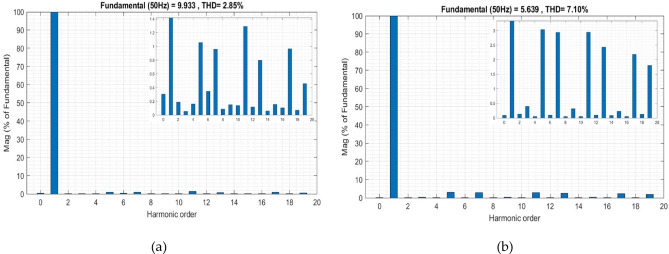 Figure 10
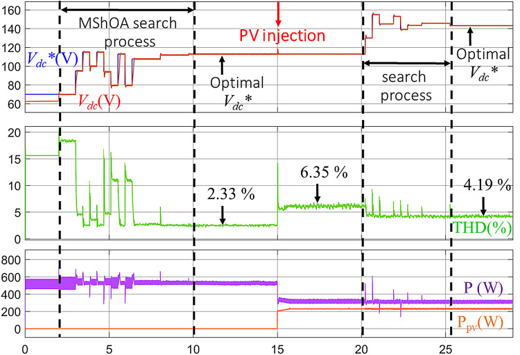 Figure 11
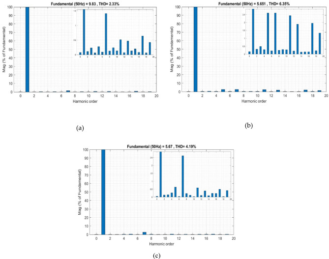 Figure 12
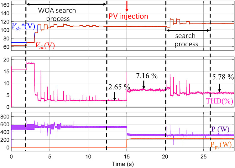 Figure 13
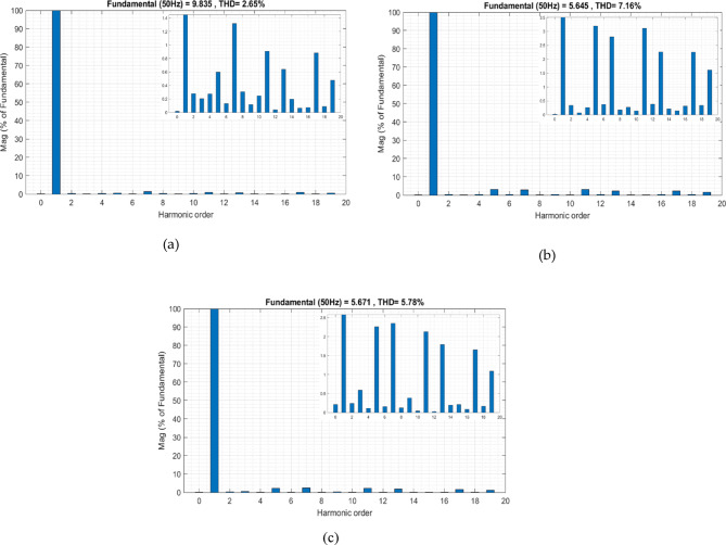 Figure 14
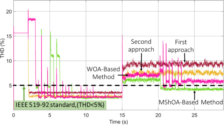 Figure 15
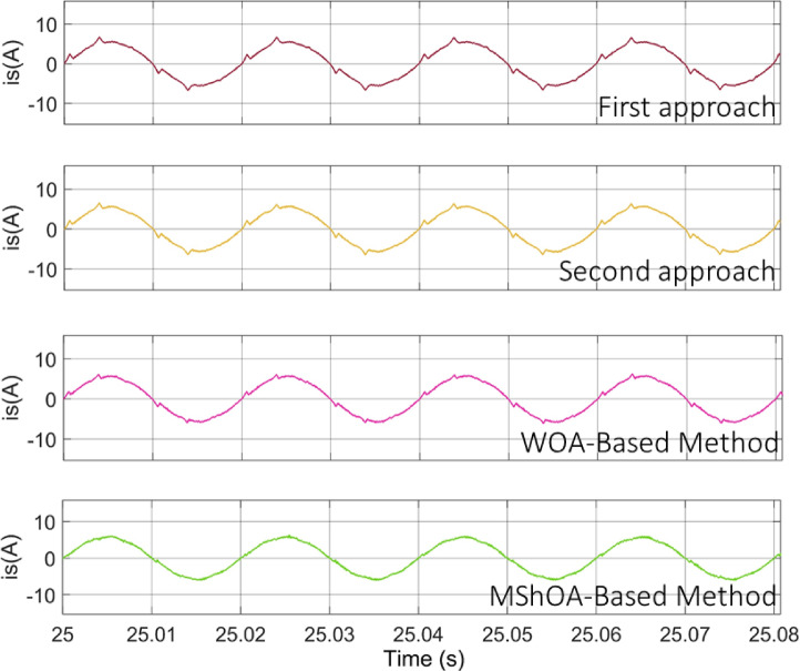 Figure 16
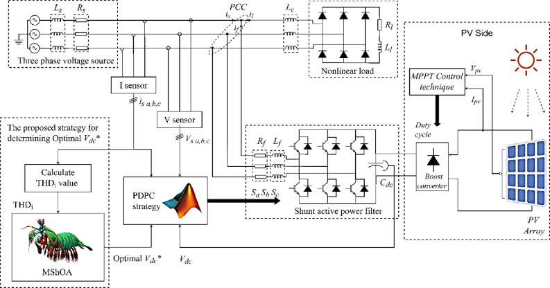 Figure 1
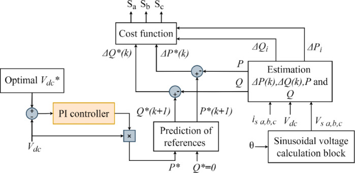 Figure 2
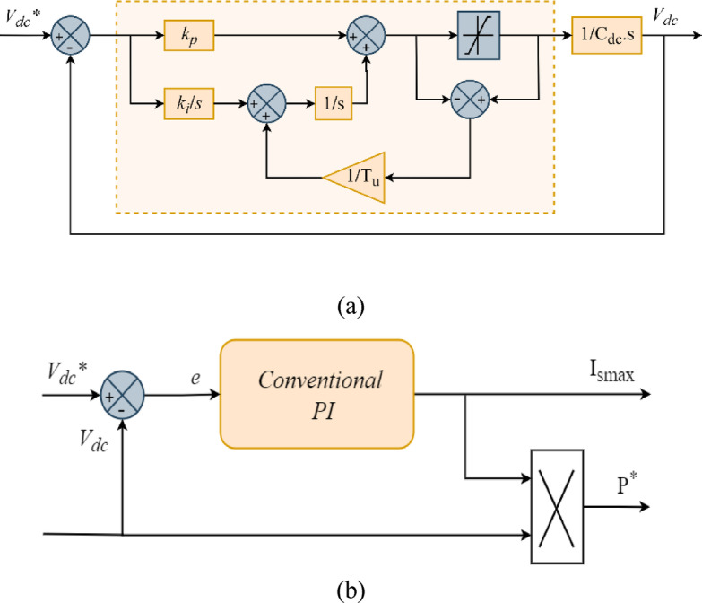 Figure 3
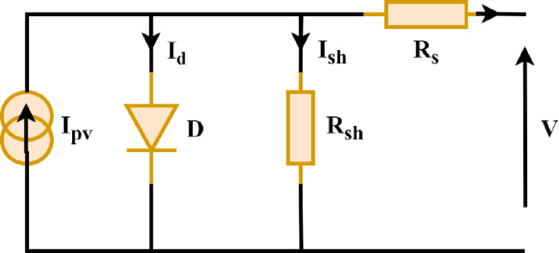 Figure 4
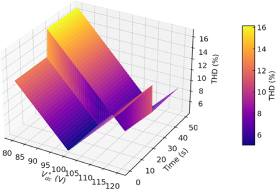 Figure 5
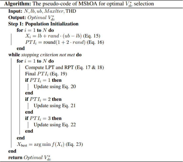 Figure 6
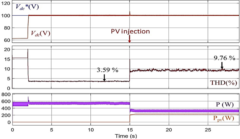 Figure 7
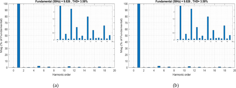 Figure 8
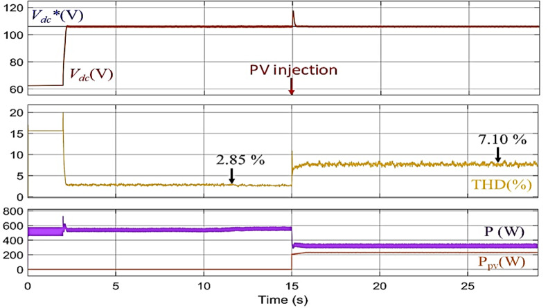 Figure 9
Peer Reviews
No public reviews on file for this paper yet. If you reviewed it on a platform where reviews are public (OpenReview, ICLR, NeurIPS, ICML), you can paste yours below so the community can read it here.
Videos
No videos yet. Explain this paper in a talk, walkthrough, or lecture? Add one.
Taxonomy
TopicsOptimal Power Flow Distribution · Microgrid Control and Optimization · Power System Optimization and Stability
Introduction
The integration of renewable energy sources, particularly photovoltaic (PV) power systems, into the electrical grid has led to a noticeable increase in harmonics, undesirable distortions in voltage and current waveforms, and a decrease in power factor, which weakens power quality. Due to the intermittent nature of solar irradiation, the energy input from PV sources to the grid can fluctuate significantly over short time periods, which may cause difficulties in maintaining grid stability^1^. Moreover, in PV systems, environmental variations such as partial shading can create multiple local maxima in the power-voltage curve, complicating the tracking of the global maximum power point. Metaheuristic optimization algorithms, such as Particle Swarm Optimization (PSO) and Whale Optimization Algorithm (WOA), have shown strong capability in overcoming such nonlinear challenges, further demonstrating their relevance for improving control performance in PV systems. To address these negative phenomena associated with PV power injection, especially in systems that contain nonlinear loads, the Shunt Active Power Filter (SAPF) emerges as an effective solution for improving power quality by injecting compensating currents into the grid^2^.
Control strategies significantly influence the performance of the SAPF. The Predictive Direct Power Control (PDPC) strategy is often used due to its structural simplicity and fast response^3^. This strategy relies on calculating the instantaneous flow of active and reactive power to control the compensating currents, without the need for explicit current control loops or Pulse Width Modulation (PWM) blocks, thereby maintaining compensation quality^4^. The choice of DC bus reference voltage (Vdc) greatly affects the effectiveness and stability of the active power filter, especially under variable load conditions and power disturbances. The appropriate selection of the V_dc_ ensures sufficient voltage headroom for the Voltage Source Inverter (VSI) to generate the necessary compensating current waveforms that oppose the harmonic currents and reactive power components generated by nonlinear loads^5^. If the value of Vdc*** is set lower than what is suitable for the system, the inverter cannot produce the required output current, particularly in high harmonic content conditions, leading to degradation in filtering performance and an increase in Total Harmonic Distortion (THD). In extreme cases, the inverter may completely lose its ability to inject compensating currents. On the other hand, a significant increase in the value of Vdc*** raises the voltage stress on power electronic components such as IGBT or MOSFET transistors, increasing the likelihood of thermal failures and reducing the overall reliability of the system. Moreover, high DC voltages lead to increased switching losses and Electromagnetic Interference (EMI), which reduces the energy efficiency of the SAPF and necessitates stricter solutions for thermal management. Therefore, the value of Vdc*** must be considered carefully to achieve a balance between providing sufficient dynamic range for harmonic compensation and minimizing energy losses and stress on power electronic components^6^.
Literature review and motivation
The DC bus voltage (Vdc) is regulated using a PI controller. However, the efficiency of the controller is highly sensitive to the reference voltage value Vdc. The injection of PV power into the grid causes dynamic disturbances, these disturbances directly affect the DC link voltage and may cause instability in its regulation if V_dc_ is not properly adjusted in real time. This leads to an increase in harmonic content and a reduction in the overall power factor. To address these issues. The research^7^ proposed an Equilibrium Optimized (EO) PI controller to regulate the Vdc in grid connected PV systems. The EO algorithm was employed to minimize Vdc variations during dynamic conditions, such as irregular PV power generation caused by insolation fluctuations. While the technique showed improved THD and power factor compared to traditional methods, its controller tuning was performed offline, limiting adaptability to real-time changes. Additionally, this study focused mainly on improving the performance of the controller itself, ignoring the impact of the Vdc*** on the overall system performance, resulting in reduced voltage error and improved power quality under dynamic disturbances. In^8^, a robust control strategy was proposed to regulate the Vdc of shunt active power filters without requiring load current measurements. The method, based on adaptive pole placement combined with a variable structure control scheme. However, the approach assumes a fixed Vdc*** and does not address the sensitivity of system performance to its value. This limitation may lead to suboptimal harmonic compensation and power quality degradation under varying operating conditions, particularly in systems with high PV penetration, where real-time adaptation of Vdc*** becomes essential. In contrast, the research^9^ introduced a theoretical approach to determine the appropriate value of Vdc, relying on the system’s load capacity and the highest-order harmonic to be compensated. Although systematic, this method neglected essential factors such as the internal resistance of the SAPF, which affected the precision of the calculated V_dc*_.* Moreover, some techniques rely on parameters such as the Maximum Filter Terminal Voltage \documentclass[12pt]{minimal} \usepackage{amsmath} \usepackage{wasysym} \usepackage{amsfonts} \usepackage{amssymb} \usepackage{amsbsy} \usepackage{mathrsfs} \usepackage{upgreek} \setlength{\oddsidemargin}{-69pt} \begin{document}$$({V_f}_{ - \max })$$\end{document} that are typically obtained through simulations, making them highly sensitive to environmental changes and system reconfigurations. Such dependencies can result in inaccurate estimation of the Vdc***, ultimately impairing the effectiveness of harmonic compensation and degrading overall power quality.
Despite these contributions, several critical research gaps remain unaddressed and are the focus of the present study:
- Poor performance under dynamic conditions: Most existing analytical approaches for determining Vdc*** are designed with fixed parameters and do not adapt in real time to variations caused by nonlinear loads or renewable energy injections.
- Neglect of Vdc*** optimization in controller design: While previous research has focused on adjusting the gains of PI controllers using intelligent algorithms, the optimal selection of Vdc*** itself remains insufficiently explored.
- Insufficient consideration of real-time power quality indicators: Previous strategies often fail to incorporate real-time indicators, such as THD, as part of the control strategy to determine Vdc***. limiting the system’s responsiveness to actual power quality conditions.
- Limited validation in realistic disturbance scenarios: Many studies validate their approaches only under steady-state conditions, without taking into account the grid disturbances common in PV integrated environments.
In response to these identified gaps, the present work proposes a real-time Vdc*** optimization strategy by leveraging the Mantis Shrimp Optimization Algorithm (MShOA), aiming to enhance the harmonic mitigation and power quality performance of SAPF.
Contributions and framework
Considering the abovementioned challenges in view, particularly those arising from the dynamic behavior of PV power injection, this research makes the following key contributions:
- Development of a novel real-time optimization strategy for dynamically adjusting the Vdc*** in a three-phase SAPF, using the MShOA. This strategy includes an online adaptive mechanism that continuously selects the optimal Vdc*** based on real-time THD feedback.
- A comparative evaluation with existing theoretical approaches for determining Vdc***, highlighting the superior performance of the proposed strategy in reducing THD and maintaining power quality.
- An additional evaluation of control efficiency, in which the proposed method is benchmarked against the WOA, highlighting enhanced convergence behavior and adaptability.
- Comprehensive simulation-based validation, demonstrating the robustness of the proposed method under PV conditions.
The remaining sections of this paper are organized as follows: Section II presents the overall system configuration and control structure of the SAPF. Section III discusses the influence of PV power injection on the stability of the Vdc. Section IV introduces the proposed approach for selecting the optimal Vdc*** using the MShOA. Section V illustrates the simulation results obtained under various operating scenarios. Section VI provides a comparative evaluation between traditional methods and the proposed technique. Finally, Section VII concludes the paper and outlines future research directions.
System description
The system integrates PV power with the electrical grid, as shown in Fig. 1, focusing on improving power quality and reducing harmonic distortions caused by nonlinear loads. This is achieved using SAPF. The harmonic components present in the load current \documentclass[12pt]{minimal} \usepackage{amsmath} \usepackage{wasysym} \usepackage{amsfonts} \usepackage{amssymb} \usepackage{amsbsy} \usepackage{mathrsfs} \usepackage{upgreek} \setlength{\oddsidemargin}{-69pt} \begin{document}$${i_l}\left( t \right)$$\end{document} , as shown in Eq. (1), significantly contribute to the THD, which can be measured using Eq. (2). The SAPF generates a compensating current \documentclass[12pt]{minimal} \usepackage{amsmath} \usepackage{wasysym} \usepackage{amsfonts} \usepackage{amssymb} \usepackage{amsbsy} \usepackage{mathrsfs} \usepackage{upgreek} \setlength{\oddsidemargin}{-69pt} \begin{document}$${i_f}\left( t \right)$$\end{document} aimed at reducing these harmonic components, ensuring that the source current \documentclass[12pt]{minimal} \usepackage{amsmath} \usepackage{wasysym} \usepackage{amsfonts} \usepackage{amssymb} \usepackage{amsbsy} \usepackage{mathrsfs} \usepackage{upgreek} \setlength{\oddsidemargin}{-69pt} \begin{document}$${i_s}\left( t \right)$$\end{document} remains as close as possible to a pure sinusoidal waveform^10^.
Fig. 1. Configuration of the studied system.
\documentclass[12pt]{minimal} \usepackage{amsmath} \usepackage{wasysym} \usepackage{amsfonts} \usepackage{amssymb} \usepackage{amsbsy} \usepackage{mathrsfs} \usepackage{upgreek} \setlength{\oddsidemargin}{-69pt} \begin{document}$${i_l}\left( t \right)={i_1}\sin \left( {\omega t+{\varphi _1}} \right)+\sum\limits_{{n=2}}^{\infty } {{i_n}} \sin \left( {n\omega t+{\varphi _n}} \right)$$\end{document}Where:
\documentclass[12pt]{minimal} \usepackage{amsmath} \usepackage{wasysym} \usepackage{amsfonts} \usepackage{amssymb} \usepackage{amsbsy} \usepackage{mathrsfs} \usepackage{upgreek} \setlength{\oddsidemargin}{-69pt} \begin{document}$${i_1}$$\end{document} Fundamental current at frequency ,
\documentclass[12pt]{minimal} \usepackage{amsmath} \usepackage{wasysym} \usepackage{amsfonts} \usepackage{amssymb} \usepackage{amsbsy} \usepackage{mathrsfs} \usepackage{upgreek} \setlength{\oddsidemargin}{-69pt} \begin{document}$${i_n}$$\end{document} Current harmonic at frequency ,
\documentclass[12pt]{minimal} \usepackage{amsmath} \usepackage{wasysym} \usepackage{amsfonts} \usepackage{amssymb} \usepackage{amsbsy} \usepackage{mathrsfs} \usepackage{upgreek} \setlength{\oddsidemargin}{-69pt} \begin{document}$${\varphi _n}$$\end{document} Phase shift of each harmonic component.
\documentclass[12pt]{minimal} \usepackage{amsmath} \usepackage{wasysym} \usepackage{amsfonts} \usepackage{amssymb} \usepackage{amsbsy} \usepackage{mathrsfs} \usepackage{upgreek} \setlength{\oddsidemargin}{-69pt} \begin{document}$$THD=\frac{{\sqrt {\sum\nolimits_{{n=2}}^{\infty } {I_{n}^{2}} } }}{{{I_1}}} \times 100\%$$\end{document}The control technique is a fundamental element in enhancing the performance of the SAPF, as it is carefully selected to ensure the highest levels of efficiency in improving power quality^11^.
PDPC control strategy
Predictive Direct Power Control (PDPC) is considered one of the most effective control techniques for improving the performance of SAPF. The PDPC strategy relies on predicting changes in active power (P) and reactive power (Q) at each time instant. The overall structure of the PDPC-based control algorithm is illustrated in Fig. 2. This schematic diagram presents the interaction between the PI controller, the reference voltage optimization block, the power prediction module, and the cost function evaluation, highlighting the sequential flow of control signals within the SAPF system.
Fig. 2. Overall structure of the PDPC control strategy.
The cost function in this strategy compares the total of active and reactive powers with their predicted values to ascertain the ideal action that minimizes tracking errors and ensures the system’s optimal performance^12^, as seen in Eq. (3).
\documentclass[12pt]{minimal} \usepackage{amsmath} \usepackage{wasysym} \usepackage{amsfonts} \usepackage{amssymb} \usepackage{amsbsy} \usepackage{mathrsfs} \usepackage{upgreek} \setlength{\oddsidemargin}{-69pt} \begin{document}$${J_i}={(\Delta {P_i})^2}+{(\Delta {Q_i})^2}$$\end{document}Where, \documentclass[12pt]{minimal} \usepackage{amsmath} \usepackage{wasysym} \usepackage{amsfonts} \usepackage{amssymb} \usepackage{amsbsy} \usepackage{mathrsfs} \usepackage{upgreek} \setlength{\oddsidemargin}{-69pt} \begin{document}$$\Delta {P_i}$$\end{document} and \documentclass[12pt]{minimal} \usepackage{amsmath} \usepackage{wasysym} \usepackage{amsfonts} \usepackage{amssymb} \usepackage{amsbsy} \usepackage{mathrsfs} \usepackage{upgreek} \setlength{\oddsidemargin}{-69pt} \begin{document}$$\Delta {Q_i}$$\end{document} represent the active and reactive power errors resulting from the application of vector \documentclass[12pt]{minimal} \usepackage{amsmath} \usepackage{wasysym} \usepackage{amsfonts} \usepackage{amssymb} \usepackage{amsbsy} \usepackage{mathrsfs} \usepackage{upgreek} \setlength{\oddsidemargin}{-69pt} \begin{document}$$\overrightarrow {{v_i}}$$\end{document} . The optimal voltage vector is chosen as follows:
\documentclass[12pt]{minimal} \usepackage{amsmath} \usepackage{wasysym} \usepackage{amsfonts} \usepackage{amssymb} \usepackage{amsbsy} \usepackage{mathrsfs} \usepackage{upgreek} \setlength{\oddsidemargin}{-69pt} \begin{document}$${\vec {v}_{{\mathrm{opt}}}}=\arg {\hbox{min} _{{{\vec {v}}_i}}}{J_i},\;\;i=0,1,...,6$$\end{document}The proposed control strategy has been shown to be effective in enhancing system performance under a variety of conditions, as previously discussed in the literature. Nevertheless, its capacity to consistently improve power quality may be restricted by its dependence on a calculated Vdc, which may not account for real-time variations in system parameters. To address this challenge, implementing an optimization method to dynamically update the V_dc_ offers significant potential for reducing THD and ensuring more stable system performance.
DC bus voltage regulation
A PI controller with anti-windup correction keeps Vdc at a steady level. The anti-windup technique is based on a second integrator with a high loop gain (1/) to stop the output from becoming too high and make sure the voltage comes back quickly. The goal of this controller is to smooth out the changes and make sure that the PDPC method works at its best. To provide a clear insight into the implementation, Fig. 3a presents the detailed anti-windup PI structure used to regulate Vdc. In addition, Fig. 3b shows how the PI controller generates the active power reference (P*), which is a key input in the PDPC control scheme for achieving effective compensation.
Fig. 3. Block diagram: (a) PI Controller with Anti-windup Compensation for Vdc Regulation, (b) Outer Control Loop for Vdc using a PI Controller.
The transfer function of the PI controller is represented by Eq. (5). Where \documentclass[12pt]{minimal} \usepackage{amsmath} \usepackage{wasysym} \usepackage{amsfonts} \usepackage{amssymb} \usepackage{amsbsy} \usepackage{mathrsfs} \usepackage{upgreek} \setlength{\oddsidemargin}{-69pt} \begin{document}$${k_P}$$\end{document} denotes the proportional constant that promptly responds to discrepancies between the actual and reference voltages, while the integral constant \documentclass[12pt]{minimal} \usepackage{amsmath} \usepackage{wasysym} \usepackage{amsfonts} \usepackage{amssymb} \usepackage{amsbsy} \usepackage{mathrsfs} \usepackage{upgreek} \setlength{\oddsidemargin}{-69pt} \begin{document}$${k_i}$$\end{document} corrects for steady state errors^13^.
\documentclass[12pt]{minimal} \usepackage{amsmath} \usepackage{wasysym} \usepackage{amsfonts} \usepackage{amssymb} \usepackage{amsbsy} \usepackage{mathrsfs} \usepackage{upgreek} \setlength{\oddsidemargin}{-69pt} \begin{document}$${H_{pi}}\left( s \right)=\frac{{{V_{dc}}}}{{{V_{dc}}*}}=\frac{{\omega _{n}^{2}}}{{{s^2}+2 \cdot \xi \cdot {\omega _n} \cdot s+{\omega _n}}}$$\end{document}The values of \documentclass[12pt]{minimal} \usepackage{amsmath} \usepackage{wasysym} \usepackage{amsfonts} \usepackage{amssymb} \usepackage{amsbsy} \usepackage{mathrsfs} \usepackage{upgreek} \setlength{\oddsidemargin}{-69pt} \begin{document}$${k_P}$$\end{document} and \documentclass[12pt]{minimal} \usepackage{amsmath} \usepackage{wasysym} \usepackage{amsfonts} \usepackage{amssymb} \usepackage{amsbsy} \usepackage{mathrsfs} \usepackage{upgreek} \setlength{\oddsidemargin}{-69pt} \begin{document}$${k_i}$$\end{document} can be calculated using Eq. (6) and Eq. (7), respectively.
\documentclass[12pt]{minimal} \usepackage{amsmath} \usepackage{wasysym} \usepackage{amsfonts} \usepackage{amssymb} \usepackage{amsbsy} \usepackage{mathrsfs} \usepackage{upgreek} \setlength{\oddsidemargin}{-69pt} \begin{document}$${k_P}=2.\xi .{\omega _n}.{C_{dc}}$$\end{document} \documentclass[12pt]{minimal} \usepackage{amsmath} \usepackage{wasysym} \usepackage{amsfonts} \usepackage{amssymb} \usepackage{amsbsy} \usepackage{mathrsfs} \usepackage{upgreek} \setlength{\oddsidemargin}{-69pt} \begin{document}$${k_i}={C_{dc}}.{\omega _n}^{2}$$\end{document}Where, \documentclass[12pt]{minimal} \usepackage{amsmath} \usepackage{wasysym} \usepackage{amsfonts} \usepackage{amssymb} \usepackage{amsbsy} \usepackage{mathrsfs} \usepackage{upgreek} \setlength{\oddsidemargin}{-69pt} \begin{document}$${\omega _n}$$\end{document} represents the natural frequency and \documentclass[12pt]{minimal} \usepackage{amsmath} \usepackage{wasysym} \usepackage{amsfonts} \usepackage{amssymb} \usepackage{amsbsy} \usepackage{mathrsfs} \usepackage{upgreek} \setlength{\oddsidemargin}{-69pt} \begin{document}$$\xi$$\end{document} denotes the damping coefficient.
To support the operation of the filter, PV power is used to supply the filter with the necessary electrical power, reducing the need for energy consumption from the main grid.
Modeling of PV system
The PV cell is the fundamental unit in PV systems. It can be represented by several mathematical models, with the single-diode model, as shown in Fig. 4, being the most common. This model is represented by Eq. (8)^14^.
\documentclass[12pt]{minimal} \usepackage{amsmath} \usepackage{wasysym} \usepackage{amsfonts} \usepackage{amssymb} \usepackage{amsbsy} \usepackage{mathrsfs} \usepackage{upgreek} \setlength{\oddsidemargin}{-69pt} \begin{document}$${I_{pv}}={I_{ph}} - {I_{str}}\left( {{e^{\frac{{V+I{R_S}}}{{n{V_t}}}}} - 1} \right) - \frac{{V+I{R_S}}}{{{R_{sh}}}}$$\end{document}Fig. 4. Single-diode equivalent circuit model of a PV Cell.
Solar cells are connected in series and parallel to form a photovoltaic array. Uniform solar irradiation of 600 W/m² is incident on the PV array, resulting in a power-voltage (P-V) curve with a single peak representing the Maximum Power Point (MPP). This study employed the Perturb and Observe (P&O) to optimize the performance of Maximum Power Point Tracking (MPPT)^15^, which facilitates the extraction of maximum available power^16^.
Impact of PV power integration on DC-link voltage stability
The integration of PV systems with the grid provides a high energy level in the system, which raises several technical challenges affecting power quality. Among the most significant challenges is maintaining the stability of the Vdc under these dynamic conditions^17^. When the system is in a stable state without PV power injection, the DC-link power balance is:
\documentclass[12pt]{minimal} \usepackage{amsmath} \usepackage{wasysym} \usepackage{amsfonts} \usepackage{amssymb} \usepackage{amsbsy} \usepackage{mathrsfs} \usepackage{upgreek} \setlength{\oddsidemargin}{-69pt} \begin{document}$${P_{in,0}}={P_{out,0}}$$\end{document}Where, \documentclass[12pt]{minimal} \usepackage{amsmath} \usepackage{wasysym} \usepackage{amsfonts} \usepackage{amssymb} \usepackage{amsbsy} \usepackage{mathrsfs} \usepackage{upgreek} \setlength{\oddsidemargin}{-69pt} \begin{document}$${P_{in,0}}$$\end{document} represents the power input to the DC-link from the DC source, while \documentclass[12pt]{minimal} \usepackage{amsmath} \usepackage{wasysym} \usepackage{amsfonts} \usepackage{amssymb} \usepackage{amsbsy} \usepackage{mathrsfs} \usepackage{upgreek} \setlength{\oddsidemargin}{-69pt} \begin{document}$${P_{out,0}}$$\end{document} denotes the power drawn from the DC-link by the inverter.
The introduction of a PV source results in the injection of additional Ppv into the grid, leading to a power imbalance, as expressed in Eq. (10):
\documentclass[12pt]{minimal} \usepackage{amsmath} \usepackage{wasysym} \usepackage{amsfonts} \usepackage{amssymb} \usepackage{amsbsy} \usepackage{mathrsfs} \usepackage{upgreek} \setlength{\oddsidemargin}{-69pt} \begin{document}$${P_{in,new}}={P_{in,0}}+{P_{pv}}$$\end{document}If there is no immediate adjustment in the \documentclass[12pt]{minimal} \usepackage{amsmath} \usepackage{wasysym} \usepackage{amsfonts} \usepackage{amssymb} \usepackage{amsbsy} \usepackage{mathrsfs} \usepackage{upgreek} \setlength{\oddsidemargin}{-69pt} \begin{document}$${P_{out,0}}$$\end{document} , the Vdc increases due to excess energy accumulating in the DC-link capacitor (Cdc). This can be expressed using the Eq. (11):
\documentclass[12pt]{minimal} \usepackage{amsmath} \usepackage{wasysym} \usepackage{amsfonts} \usepackage{amssymb} \usepackage{amsbsy} \usepackage{mathrsfs} \usepackage{upgreek} \setlength{\oddsidemargin}{-69pt} \begin{document}$$\frac{d}{{dt}}\left( {\frac{1}{2}{C_{dc}}V_{{dc}}^{2}} \right)={P_{in,new}} - {P_{out,new}}$$\end{document}Where, \documentclass[12pt]{minimal} \usepackage{amsmath} \usepackage{wasysym} \usepackage{amsfonts} \usepackage{amssymb} \usepackage{amsbsy} \usepackage{mathrsfs} \usepackage{upgreek} \setlength{\oddsidemargin}{-69pt} \begin{document}$${P_{out,new}}$$\end{document} represents the new power drawn from the DC-link by the inverter after the injection of Ppv. If \documentclass[12pt]{minimal} \usepackage{amsmath} \usepackage{wasysym} \usepackage{amsfonts} \usepackage{amssymb} \usepackage{amsbsy} \usepackage{mathrsfs} \usepackage{upgreek} \setlength{\oddsidemargin}{-69pt} \begin{document}$${P_{out}}$$\end{document} is not adjusted, the accumulated energy causes a rise in Vdc, resulting in a new ideal Vdc***:
\documentclass[12pt]{minimal} \usepackage{amsmath} \usepackage{wasysym} \usepackage{amsfonts} \usepackage{amssymb} \usepackage{amsbsy} \usepackage{mathrsfs} \usepackage{upgreek} \setlength{\oddsidemargin}{-69pt} \begin{document}$$V_{{dc,new}}^{*}\left( {optimal} \right)>V_{{dc,0}}^{*}\left( {optimal} \right)$$\end{document}This imbalance in power leads to an increase in the Vdc value, causing a rise in THD due to rapid voltage fluctuations. Figure 5 presents a heat map that helps illustrate the impact of Vdc*** on power quality in grid-connected PV systems. Before injecting PV power, an optimal value of Vdc*** is clearly observed, corresponding to the lowest THD. However, after PV power injection, this optimal Vdc*** shifts to a higher value than before. This change occurs due to variations in power flow within the system and its effect on the energy balance at the DC link.
Fig. 5. Heat map illustrating the impact of Vdc*** on THD before and after PV power injection.
The impact of the Vdc*** value on system quality highlights the need to determine this value accurately to maintain a minimum of harmonic distortions.
Optimal DC bus reference voltage selection in PV systems
In this study, two conventional methods are applied to calculate the Vdc*** in a SAPF system when integrating PV power, and the impact of each method on system quality is analyzed. Subsequently, a new technique is proposed to determine the optimal Vdc*** with higher accuracy, and its effectiveness is evaluated by comparing it with conventional methods.
Traditional methods for calculating the DC bus reference voltage
In previous studies, approximate methods based on mathematical equations have been used to calculate the value of Vdc. These equations rely on a set of fundamental system parameters, including the source voltage (V_s). For example, the value of Vdc_ is calculated according to the first method using Eq. (13)^18^:
\documentclass[12pt]{minimal} \usepackage{amsmath} \usepackage{wasysym} \usepackage{amsfonts} \usepackage{amssymb} \usepackage{amsbsy} \usepackage{mathrsfs} \usepackage{upgreek} \setlength{\oddsidemargin}{-69pt} \begin{document}$${V_{dc}}*=\frac{{2\sqrt 2 }}{{1.155}} \cdot {V_{s(LL)}}$$\end{document}Additionally, there are other methods to determine the value of Vdc*** that require data extracted from simulations, such as the inverter output voltage (Vf−max) value. In the second method, Eq. (14) illustrates how to calculate the value of Vdc***, providing a different approach based on the system’s operational characteristics^16^.
\documentclass[12pt]{minimal} \usepackage{amsmath} \usepackage{wasysym} \usepackage{amsfonts} \usepackage{amssymb} \usepackage{amsbsy} \usepackage{mathrsfs} \usepackage{upgreek} \setlength{\oddsidemargin}{-69pt} \begin{document}$${V_{dc}}*=\sqrt 3 \cdot {V_{f\_\hbox{max} }}$$\end{document}Despite the effectiveness of these traditional methods, they lack the ability to adapt to dynamic changes in the grid, which are exemplified by the injection of PV power. This is due to the reliance of these traditional methods on fixed mathematical models for determining the Vdc***, making them less efficient in handling sudden changes that the system may experience.
Vdc* optimization using mantis shrimp optimization algorithm (MShOA)
Given the PV energy injection into the SAPF system, and the resulting fluctuations that affect the stability of Vdc, the Mantis Shrimp Optimization Algorithm (MShOA) is dynamically adapt to the Vdc. This metaheuristic algorithm is inspired by the complex visual system of this marine creature, which has exceptional light polarization analysis capabilities. The algorithm relies on three intelligent behaviors: foraging, attacking, and sheltering. Its primary goal is to minimize the THD in the grid current by instantly selecting the optimal value for the V_dc_.
The following steps are used to implement the MAShA algorithm for Vdc*** optimization in real time:
- A.Population initialization.
An initial population of solutions \documentclass[12pt]{minimal} \usepackage{amsmath} \usepackage{wasysym} \usepackage{amsfonts} \usepackage{amssymb} \usepackage{amsbsy} \usepackage{mathrsfs} \usepackage{upgreek} \setlength{\oddsidemargin}{-69pt} \begin{document}$${X_i}$$\end{document} is generated for =1,2,…,, within a defined search range bounded by \documentclass[12pt]{minimal} \usepackage{amsmath} \usepackage{wasysym} \usepackage{amsfonts} \usepackage{amssymb} \usepackage{amsbsy} \usepackage{mathrsfs} \usepackage{upgreek} \setlength{\oddsidemargin}{-69pt} \begin{document}$$lb$$\end{document} and \documentclass[12pt]{minimal} \usepackage{amsmath} \usepackage{wasysym} \usepackage{amsfonts} \usepackage{amssymb} \usepackage{amsbsy} \usepackage{mathrsfs} \usepackage{upgreek} \setlength{\oddsidemargin}{-69pt} \begin{document}$$ub$$\end{document} :
\documentclass[12pt]{minimal} \usepackage{amsmath} \usepackage{wasysym} \usepackage{amsfonts} \usepackage{amssymb} \usepackage{amsbsy} \usepackage{mathrsfs} \usepackage{upgreek} \setlength{\oddsidemargin}{-69pt} \begin{document}$${X_i}=lb+rand \cdot (ub - lb)$$\end{document}Additionally, an initial Polarization Type Indicator (PTI) is assigned to each individual \documentclass[12pt]{minimal} \usepackage{amsmath} \usepackage{wasysym} \usepackage{amsfonts} \usepackage{amssymb} \usepackage{amsbsy} \usepackage{mathrsfs} \usepackage{upgreek} \setlength{\oddsidemargin}{-69pt} \begin{document}$${X_i}$$\end{document} :
\documentclass[12pt]{minimal} \usepackage{amsmath} \usepackage{wasysym} \usepackage{amsfonts} \usepackage{amssymb} \usepackage{amsbsy} \usepackage{mathrsfs} \usepackage{upgreek} \setlength{\oddsidemargin}{-69pt} \begin{document}$$PT{I_i}={\mathrm{round}}(1+2 \cdot rand)$$\end{document}- B.Eye angle and polarization type computation.
To ascertain the polarization type detected by each eye, two polarization angles are computed, the left polarization angle (LPA) is calculated, which is determined by its similarity to the optimal solution, and the Right Polarization Angle (RPA), which is generated arbitrarily. The Left Angular Deviation (LAD) and Right Angular Deviation (RAD) are calculated by the algorithm from these values, which assess the degree to which each angle corresponds to predetermined polarization directions. The dominant eye is then identified for decision-making by comparing these deviations.
Then, the polarization types are assigned as follows^19^:
LPT:
\documentclass[12pt]{minimal} \usepackage{amsmath} \usepackage{wasysym} \usepackage{amsfonts} \usepackage{amssymb} \usepackage{amsbsy} \usepackage{mathrsfs} \usepackage{upgreek} \setlength{\oddsidemargin}{-69pt} \begin{document}$$LPT=\;\;\;{\kern 1pt} \left\{ {\begin{array}{*{20}{l}} {1,}&{{\mathrm{if}}\;\;\;{\kern 1pt} \frac{{3\pi }}{8} \leqslant LPA \leqslant \frac{{5\pi }}{8}}&{} \\ {2,}&{{\mathrm{if}}\;\;\;{\kern 1pt} 0 \leqslant LPA \leqslant \frac{\pi }{8}\;\;\;{\kern 1pt} {\mathrm{or}}\;\;\;{\kern 1pt} \frac{{7\pi }}{8} \leqslant LPA \leqslant \pi }&{} \\ {3,}&{{\mathrm{if}}\;\;\;{\kern 1pt} \frac{\pi }{8}<LPA<\frac{{3\pi }}{8}\;\;\;{\kern 1pt} {\mathrm{or}}\;\;\;{\kern 1pt} \frac{{5\pi }}{8}<LPA<\frac{{7\pi }}{8}}&{} \end{array}} \right.$$\end{document}RPT:
\documentclass[12pt]{minimal} \usepackage{amsmath} \usepackage{wasysym} \usepackage{amsfonts} \usepackage{amssymb} \usepackage{amsbsy} \usepackage{mathrsfs} \usepackage{upgreek} \setlength{\oddsidemargin}{-69pt} \begin{document}$$RPT=\;\;\;{\kern 1pt} \left\{ {\begin{array}{*{20}{l}} {1,}&{{\mathrm{if}}\;\;\;{\kern 1pt} \frac{{3\pi }}{8} \leqslant RPA \leqslant \frac{{5\pi }}{8}}&{} \\ {2,}&{{\mathrm{if}}\;\;\;{\kern 1pt} 0 \leqslant RPA \leqslant \frac{\pi }{8}\;\;\;{\kern 1pt} {\mathrm{or}}\;\;\;{\kern 1pt} \frac{{7\pi }}{8} \leqslant RPA \leqslant \pi }&{} \\ {3,}&{{\mathrm{if}}\;\;\;{\kern 1pt} \frac{\pi }{8}<RPA<\frac{{3\pi }}{8}\;\;\;{\kern 1pt} {\mathrm{or}}\;\;\;{\kern 1pt} \frac{{5\pi }}{8}<RPA<\frac{{7\pi }}{8}}&{} \end{array}} \right.$$\end{document}Ultimately, the effective polarization type (PTI) is determined by the lesser angular deviation:
\documentclass[12pt]{minimal} \usepackage{amsmath} \usepackage{wasysym} \usepackage{amsfonts} \usepackage{amssymb} \usepackage{amsbsy} \usepackage{mathrsfs} \usepackage{upgreek} \setlength{\oddsidemargin}{-69pt} \begin{document}$$PT{I_i}=\left\{ {\begin{array}{*{20}{l}} {LP{T_i}}&{{\mathrm{if}}LA{D_i}<RA{D_i}}&{} \\ {RP{T_i}}&{{\mathrm{if}}LA{D_i}>RA{D_i}}&{} \end{array}} \right.$$\end{document}- C.Position update based on behavior.
According to the value of PTI, each individual’s position is updated using one of the following behavioral rules:
If PTI = 1 (Foraging behavior):
\documentclass[12pt]{minimal} \usepackage{amsmath} \usepackage{wasysym} \usepackage{amsfonts} \usepackage{amssymb} \usepackage{amsbsy} \usepackage{mathrsfs} \usepackage{upgreek} \setlength{\oddsidemargin}{-69pt} \begin{document}$$\begin{gathered} X_{i}^{{t+1}}={X_{best}} - v \cdot {\mathrm{rand}} \cdot ({X_r} - X_{i}^{t}),\;\;\;{\kern 1pt} rand \in [ - 1,1] \hfill \\ v=X_{i}^{t} - {X_{best}} \hfill \\ \end{gathered}$$\end{document}If PTI = 2 (Attacking behavior):
\documentclass[12pt]{minimal} \usepackage{amsmath} \usepackage{wasysym} \usepackage{amsfonts} \usepackage{amssymb} \usepackage{amsbsy} \usepackage{mathrsfs} \usepackage{upgreek} \setlength{\oddsidemargin}{-69pt} \begin{document}$$X_{i}^{{t+1}}={X_{best}} \cdot \cos \theta$$\end{document}If PTI = 3 (Sheltering behavior):
\documentclass[12pt]{minimal} \usepackage{amsmath} \usepackage{wasysym} \usepackage{amsfonts} \usepackage{amssymb} \usepackage{amsbsy} \usepackage{mathrsfs} \usepackage{upgreek} \setlength{\oddsidemargin}{-69pt} \begin{document}$$\begin{gathered} X_{i}^{{t+1}}={x_{best}}+rand \cdot ({x_{best}}),\;\;\;{\kern 1pt} rand \in [0,0.3] \hfill \\ X_{i}^{{t+1}}={x_{best}} - rand \cdot ({x_{best}}),\;\;\;{\kern 1pt} rand \in [0,0.3] \hfill \\ \end{gathered}$$\end{document}Where:
\documentclass[12pt]{minimal} \usepackage{amsmath} \usepackage{wasysym} \usepackage{amsfonts} \usepackage{amssymb} \usepackage{amsbsy} \usepackage{mathrsfs} \usepackage{upgreek} \setlength{\oddsidemargin}{-69pt} \begin{document}$$X_{i}^{t}$$\end{document} The current position of the \documentclass[12pt]{minimal} \usepackage{amsmath} \usepackage{wasysym} \usepackage{amsfonts} \usepackage{amssymb} \usepackage{amsbsy} \usepackage{mathrsfs} \usepackage{upgreek} \setlength{\oddsidemargin}{-69pt} \begin{document}$${i^{th}}$$\end{document} ith individual at iteration t,
\documentclass[12pt]{minimal} \usepackage{amsmath} \usepackage{wasysym} \usepackage{amsfonts} \usepackage{amssymb} \usepackage{amsbsy} \usepackage{mathrsfs} \usepackage{upgreek} \setlength{\oddsidemargin}{-69pt} \begin{document}$$X_{i}^{{t+1}}$$\end{document} The updated position,
\documentclass[12pt]{minimal} \usepackage{amsmath} \usepackage{wasysym} \usepackage{amsfonts} \usepackage{amssymb} \usepackage{amsbsy} \usepackage{mathrsfs} \usepackage{upgreek} \setlength{\oddsidemargin}{-69pt} \begin{document}$${x_{best}}$$\end{document} The best solution,
\documentclass[12pt]{minimal} \usepackage{amsmath} \usepackage{wasysym} \usepackage{amsfonts} \usepackage{amssymb} \usepackage{amsbsy} \usepackage{mathrsfs} \usepackage{upgreek} \setlength{\oddsidemargin}{-69pt} \begin{document}$${X_r}$$\end{document} A randomly selected individual from the population,
\documentclass[12pt]{minimal} \usepackage{amsmath} \usepackage{wasysym} \usepackage{amsfonts} \usepackage{amssymb} \usepackage{amsbsy} \usepackage{mathrsfs} \usepackage{upgreek} \setlength{\oddsidemargin}{-69pt} \begin{document}$$rand$$\end{document} A uniformly distributed random number.
This mechanism enables the algorithm to adaptively explore and exploit the search space in accordance with the behavior dictated by PTI.
- D.Evaluation and best solution selection.
The objective function value (THD level) for all individuals is assessed during each iteration. The optimal candidate solution is revised in accordance with:
\documentclass[12pt]{minimal} \usepackage{amsmath} \usepackage{wasysym} \usepackage{amsfonts} \usepackage{amssymb} \usepackage{amsbsy} \usepackage{mathrsfs} \usepackage{upgreek} \setlength{\oddsidemargin}{-69pt} \begin{document}$${X_{{\mathrm{best}}}}=\arg \hbox{min} \cdot f({X_i})$$\end{document}This process repeats until a maximum number of iterations is reached or a minimum THD value is achieved. Finally, the optimal solution \documentclass[12pt]{minimal} \usepackage{amsmath} \usepackage{wasysym} \usepackage{amsfonts} \usepackage{amssymb} \usepackage{amsbsy} \usepackage{mathrsfs} \usepackage{upgreek} \setlength{\oddsidemargin}{-69pt} \begin{document}$${X_{{\mathrm{best}}}}$$\end{document} is adopted as the final Vdc*** used in the SAPF system. To provide a clearer view of the implementation procedure, the pseudo-code corresponding to the proposed MShOA-based is presented in Fig. 6.
Fig. 6. Pseudo-code of the MShOA for Optimal Vdc*** Determination in SAPF.
Simulation results
This section presents a series of simulation results to study the effect of the Vdc* value in the SAPF system under the influence of PV energy injection. To accurately capture the harmonic dynamics and switching behavior of the system, a detailed switching model of the three-phase VSI and SAPF was used, incorporating Pulse Width Modulation (PWM) and nonlinear load modeling. The simulation is designed to reflect realistic operating conditions, and all simulations were performed in the MATLAB/Simulink environment using the system parameters shown in Table 1.
Table 1. System’s parameters.ParametersValuesGrid SideSource voltage Vs25 VSource resistance RS0.1 ΩSource inductance Ls0. 1 mHSupply frequency f50 HzDC Bus reference voltage (Approach 1) Vdc^^ _APP1_100 VDC Bus reference voltage (Approach 2) V_dc_^^ APP2_106 VDC Bus reference voltage (IGWO) Vdc^**^ _MShOA* (Before injecting PV power)113.5 VDC Bus reference voltage (IGWO) Vdc^**^ _MShOA_ (After injecting PV power)147.8 VDC Bus capacitor C_dc_1100 µFFilter inductance L_f8.5 mHFilter resistance Rf0.1 ΩProportional gain kp0.1521Integral gain ki2.1713Sampling time Ts4.5 µsLoad inductance Ll8.5 mHLoad resistance Rl*_5 ΩPV SideOpen circuit voltage V_oc_36.6 VCourt circuit current I_cc_7.97 ACurrent at maximum power point I_mpp_7.27 AVoltage at maximum power point V_mpp_29.3 V
Traditional methods analysis
In this analysis, the efficacy of two conventional approaches utilized to determine Vdc*** in the SAPF system is assessed. It is also investigated how the Vdc*** value affects the grid current’s THD. Additionally, these two conventional approaches will be evaluated in the context of PV power injection.
The first method used Eq. (13) to obtain the correct value of Vdc*. The result was a Vdc*** value of 100 volts, As illustrated in Fig. 7. Before activating the active filter, the distortion level in the grid is high due to the absence of any effective correction for these distortions caused by nonlinear loads. THD of the current was measured at 16%. After activating the filter at T = 2 s, the Vdc closely follows its reference value Vdc* during the initial phase, maintaining a relatively stable level. Additionally, THD is effectively reduced to 3.59%, as shown in Fig. 8a. Indicating the efficiency of the PDPC technique. However, since the value of Vdc*** was calculated using the first approach, the system’s performance remains constrained by the accuracy of this method and its effectiveness under dynamic operating conditions or when external disturbances are applied to the system. at T = 15 s, a noticeable fluctuation in the Vdc curve is observed, indicating the system’s struggle to maintain stability under the dynamic conditions introduced by PV power injection. In parallel, the THD rises again to 9.76%, as illustrated in Fig. 8b., revealing a significant deterioration in power quality.
Fig. 7. Performance of the SAPF using the first conventional method before and after PV power injection.
Fig. 8. Grid current THD evolution using the first conventional method: (a) Before PV injection, (b) After PV injection.
By transitioning to the second conventional method while maintaining the same previous test conditions, the impact of the Vdc* value on the system is assessed. Initially, the Vdc* value is calculated using Eq. (13), resulting in a reference value of 106 V. As shown in Fig. 9, after activating the filter at 2 s, an improvement in the stability of the Vdc* observed, leading to a reduction in the THD to 2.85%, as illustrated in Fig. 10a. However, when PV power is injected at T = 15 s, similar challenges arise. The Vdc is affected by sudden changes, and the THD increases to 7.10%, as seen in Fig. 10b. Indicating the impact of dynamic conditions on the efficiency of the second approach. second.
Fig. 9. Performance of the SAPF using the second conventional Method before and after PV power injection.
Fig. 10. Grid current THD evolution using the second conventional method: (a) Before PV injection, (b) After PV injection.
The simulation results for both the first and second approaches for calculating the value of Vdc* reveal that their effectiveness is limited in accurately determining this value, especially under dynamic conditions or external disturbances affecting the system. This is particularly evident during PV power injection, where the THD increased significantly in both methods. In light of these findings, it becomes evident that more flexible and intelligent techniques are required, ones that can perform real-time optimization and account for power quality indicators.
Proposed technique analysis
To validate the effectiveness of the proposed optimization-based control strategy, this section presents a detailed analysis of the applied algorithms used to determine the optimal reference voltage Vdc**. Two intelligent optimization methods were considered: the MShOA, which forms the basis of the proposed approach, and the Whale Optimization Algorithm (WOA), implemented for comparison and verification purposes. Each algorithm is analyzed separately under identical operating conditions to evaluate its capability in minimizing THD and maintaining V_dc*_ stability.
Performance of the proposed MShOA-based method
To overcome the limitations of traditional methods, the proposed technique, which relies on the MShOA, was applied to dynamically determine the optimal Vdc* in real time. To ensure a fair comparison, the simulation was conducted under the same test conditions as those used for the first and second conventional approaches, including PV power injection at T = 15 s As shown in Fig. 11, the evolution of both Vdc and Vdc* over time is presented, along with their impact on the THD.
Before activating the active filter, the THD was high, and the Vdc* was unstable at its reference value Vdc. After activating the filter at T = 2 s, the MShOA initiated the search process for the optimal V_dc_. At the beginning of this process, an increase in THD is observed, which corresponds to unsuitable Vdc* values for the system. As the MShOA continued its search, the value of Vdc* was gradually adjusted, positively impacting the THD by reducing it to 2.33%, as shown in Fig. 12a. This is achieved by relying on the objective function of the MShOA, which guides the search process to select the Vdc* value that corresponds to the lowest THD.
In the second phase, PV power is injected at T = 15 s. The MShOA is programmed to restart the search process at T = 20 s to highlight the difference in THD levels before and after applying the algorithm under changing conditions. Initially, after PV injection, a significant increase in THD to 6.35% is observed, as shown in Fig. 12b. This rise in THD is attributed to the fact that the previously determined Vdc* value is no longer suitable for the system under these new conditions.
Subsequently, the MShOA begins searching for the appropriate Vdc* value that matches the new conditions. Initially, fluctuations in THD values appear, as the search process continues, the Vdc* values gradually adapt to the new operating conditions, leading to a reduction in THD to 4.19%, as illustrated in Fig. 12c. This confirms the effectiveness of the proposed technique in determining the optimal Vdc* value and its ability to dynamically adapt to real-time operating changes, thereby improving power quality efficiently under these varying conditions.
Fig. 11. Real-Time evolution of Vdc* and Vdc with the proposed MShOA under PV injection conditions.
Fig. 12THD improvement using MShOA: (a) Before PV injection, (b) After PV injection, (c) Post re-optimization.
Implementation of the Whale optimization algorithm (WOA)
To expand the scope of the analysis, the WOA was applied to determine the optimal Vdc***. The WOA mimics the bubble-net hunting behavior of humpback whales and alternates between exploration and exploitation phases to locate the optimal solution within a defined search space. In this study, the same system parameters, operating conditions, and objective function used with the MShOA were maintained to ensure consistency in evaluation.
Simulation results obtained using the WOA demonstrate its ability to converge toward a feasible Vdc*** value and effectively reduce the THD of the source current, as illustrated in Fig. 13. Before activating the active filter, the THD level was high; once the filter was activated at T = 2 s, the WOA began its optimization process, reducing the THD to 2.65%, as shown in Fig. 14a. In the second phase, when PV power was injected at T = 15 s, a noticeable increase in THD to 7.16% was observed, as illustrated in Fig. 14b. This increase occurs because the previously determined Vdc*** no longer matches the system’s new operating conditions. As the WOA continues its iterative search, Vdc*** adapts to the new conditions, resulting in a reduction of THD to 5.78%, as shown in Fig. 14c.
These results confirm the capability of the WOA to dynamically adjust Vdc*** and maintain acceptable harmonic distortion levels, although its convergence speed and final performance remain lower than those achieved with the proposed MShOA-based method.
Fig. 13. Real-Time evolution of Vdc* and Vdc with the WOA under PV injection conditions.
Fig. 14THD improvement using WOA: (a) Before PV injection, (b) After PV injection, (c) Post re-optimization.
Comparative evaluation
To validate the effectiveness of the proposed MShOA-based technique in determining the optimal value of Vdc***, a comparative analysis was conducted with another optimization-based approach using the WOA. The inclusion of the WOA method serves to further verify the superiority of the MShOA strategy under identical conditions. Additionally, two conventional methods were analyzed for reference and benchmarking purposes.
As illustrated in Fig. 15, the proposed MShOA-based technique demonstrates a distinctly superior performance compared to all other approaches. When the filter is activated at T = 2 s, the MShOA achieves the lowest THD value of 2.33%, followed by the WOA-based method at 2.65%, while the conventional techniques record significantly higher distortion levels of 3.59% and 2.85%, respectively. This initial result clearly indicates the higher precision and faster convergence of the MShOA in identifying the optimal reference voltage. During PV power injection at T = 15 s, the advantage of the MShOA becomes even more evident. While both optimization algorithms adapt to dynamic variations, the WOA-based method reduces THD to 5.78%, whereas the proposed MShOA achieves a superior reduction to 4.19%, maintaining distortion within the acceptable limit defined by the IEEE 519 − 92 standard (< 5%).
Fig. 15. Comparative Analysis of THD Reduction.
To provide a clearer quantitative comparison, Table 2 summarizes the THD values obtained for all evaluated methods, both before and after PV power injection.
Table 2THD performance comparison before and after PV injection using conventional methods, WOA, and MShOA.MethodTHD before PV injection (%)THD after PV injection (%)First traditional approach3.599.76Second traditional approach2.857.10WOA-based method2.655.78Proposed MShOA-based method2.334.19
These outcomes confirm that, although the WOA improves upon conventional approaches, the MShOA-based strategy consistently provides the best dynamic adaptability, faster optimization response, and lowest harmonic distortion, proving its higher robustness and effectiveness in real-time voltage control and power quality enhancement.
Figure 16. presents a comparison of the \documentclass[12pt]{minimal} \usepackage{amsmath} \usepackage{wasysym} \usepackage{amsfonts} \usepackage{amssymb} \usepackage{amsbsy} \usepackage{mathrsfs} \usepackage{upgreek} \setlength{\oddsidemargin}{-69pt} \begin{document}$${i_s}\left( t \right)$$\end{document} waveform after PV power injection into the system using two conventional methods, as well as two optimization-based techniques. The WOA-based approach and the proposed MShOA-based method. It is evident that the conventional methods fail to effectively correct the current waveform, as noticeable distortions remain, negatively impacting the overall power quality.
Fig. 16. Improvement of source current waveform using the proposed MShOA Technique under PV injection.
In contrast, the optimization-based approaches provide a much smoother and more sinusoidal waveform. Among them, the proposed MShOA-based technique delivers the best performance, producing a source current waveform that is the closest to the ideal sinusoidal form. This confirms its superior ability to minimize harmonic distortion and maintain stable operation under dynamic conditions, surpassing both the WOA and conventional approaches in terms of accuracy and efficiency.
Conclusion
This work presented a novel real-time optimization strategy for dynamically adjusting the DC bus reference voltage (Vdc*) in a three-phase Shunt Active Power Filter (SAPF) under photovoltaic (PV) power injection conditions. The proposed technique is based on the Mantis Shrimp Optimization Algorithm (MShOA).
The simulation results confirmed the limitations of existing approaches in adapting Vdc*** under dynamic operating conditions. Both conventional analytical methods and the Whale Optimization Algorithm (WOA) achieved acceptable performance only under steady state, but they failed to maintain power quality when sudden PV power injections introduced disturbances, leading to noticeable increases in Total Harmonic Distortion (THD) and voltage instability. In contrast, the proposed MShOA-based strategy demonstrated a superior ability to accurately and adaptively adjust Vdc* in real time, achieving lower THD values, enhanced system stability, and full compliance with IEEE 519 − 92 harmonic standards under PV injection.
Future research will explore the integration of experimental validations and hardware implementation of the proposed approach, as well as extending the optimization framework to multi-objective scenarios involving power factor correction and energy efficiency.
The reference list from the paper itself. Each links out to its DOI / PubMed record.
- 1Gu, Z., Li, B., Zhang, G. & Li, B. Optimizing photovoltaic integration in grid management via a deep learning-based scenario analysis. Sci. Rep.15(1), 14851. 10.1038/s 41598-025-98724-3.10.1038/s 41598-025-98724-3PMC 1203801640295668 · doi ↗ · pubmed ↗
- 2Annamalaichamy, A., David, P. W., Balachandran, P. K. & Colak, I. Performance evaluation of PI and FLC controller for shunt active power filters. Electr. Eng.107(1), 1235–1252. 10.1007/s 00202-024-02546-x.
- 3Boopathi, R. & Indragandhi, V. Enhancement of power quality in grid-connected systems using a predictive direct power controlled based PV-interfaced with multilevel inverter shunt active power filter. Sci. Rep.15(1), 7967. 10.1038/s 41598-025-92693-3.10.1038/s 41598-025-92693-3PMC 1188916440055504 · doi ↗ · pubmed ↗
- 4Debdouche, N., Benbouhenni, H., Deffaf, B., Anwar, G. & Zarour, L. Predictive direct power control with phase-locked loop technique of three‐level neutral point clamped inverter based shunt active power filter for power quality improvement, Circuit Theory & Apps, vol. 52, no. 7, pp. 3306–3340, Jul. (2024). 10.1002/cta.3871
- 5Srilakshmi, K. et al. Design and simulation of reduced switch converter based solar PV and energy storage fed shunt active power filter with butterfly optimization. Results Control Optim.19, 100554. 10.1016/j.rico.2025.100554.
- 6Chankaya, M., Naqvi, S. B. Q., Hussain, I., Singh, B. & Ahmad, A. Power quality enhancement and improved dynamics of a grid tied PV system using equilibrium optimization control based regulation of DC bus voltage. Electr. Power Syst. Res.226, 109911. 10.1016/j.epsr.2023.109911 (Jan. 2024).
- 7Afghoul, H., Chikouche, D., Krim, F., Babes, B. & Beddar, A. Implementation of Fractional-order Integral-plus-proportional Controller to Enhance the Power Quality of an Electrical Grid. Electr. Power Compon. Syst.44(9), 1018–1028. 10.1080/15325008.2016.1147509.
- 8Behera, R. R., Dash, A. R., Mishra, S., Panda, A. K. & Gelmecha, D. J. Implementation of a hybrid neural network control technique to a cascaded MLI based SAPF. Sci. Rep.14(1), 8614. 10.1038/s 41598-024-58137-0.10.1038/s 41598-024-58137-0PMC 1101654838616206 · doi ↗ · pubmed ↗