A modified Dung Beetle optimizer for combined heat and power economic dispatch considering power losses, valve-point effects, and operating constraints
Mahmoud Rihan, Mohamed Ebeed, Noor Habib Khan, Raheela Jamal, Mosaed Elnaka, Morsy Nour, Amal M. Abd El Hamid, Hany S. E. Mansour

TL;DR
This paper introduces a modified Dung Beetle Optimizer to solve complex power system optimization problems more efficiently.
Contribution
The novelty is proposing a modified Dung Beetle Optimizer (MDBO) with three improvement strategies for solving Combined Heat and Power Economic Dispatch problems.
Findings
The MDBO significantly reduces operating costs in Combined Heat and Power Economic Dispatch problems.
MDBO outperforms existing optimization techniques like SCSO, AVOA, and GWO in various test scenarios.
The algorithm effectively handles power losses, valve-point effects, and prohibited operating zones.
Abstract
The Combined Heat and Power Economic Dispatch (CHPED) problem represents a significant optimization challenge in modern power systems due to its inherent complexity arising from multiple operational constraints. This complexity is further exacerbated when considering the effect of power losses (PLs), valve-point loading effect (VPLE), and prohibited operating zones (POZs). Consequently, an efficient and robust optimization algorithm is essential for obtaining a globally optimal solution while satisfying all constraints. To address these challenges, this work evaluates the effectiveness of the Modified Dung Beetle Optimizer (MDBO) for solving the CHPED problem, considering PLs, VPLE, and POZs. The MDBO enhances the search process and mitigates the limitations of the conventional Dung Beetle Optimizer, particularly stagnation and premature convergence to local optima. The novelty in this…
Genes, proteins, chemicals, diseases, species, mutations and cell lines named across the full text — each resolved to its canonical identifier and authoritative record.
Click any figure to enlarge with its caption.
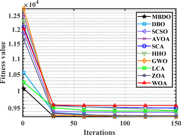 Figure 10
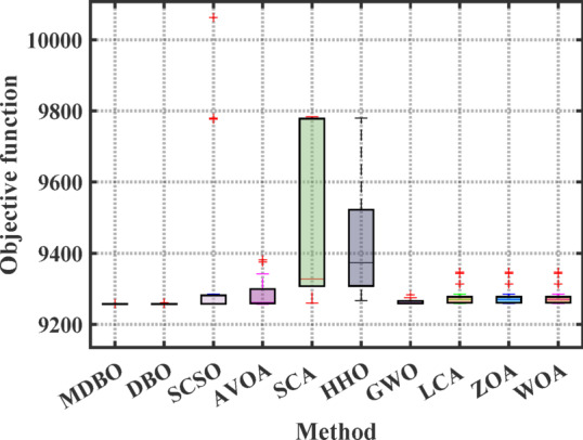 Figure 11
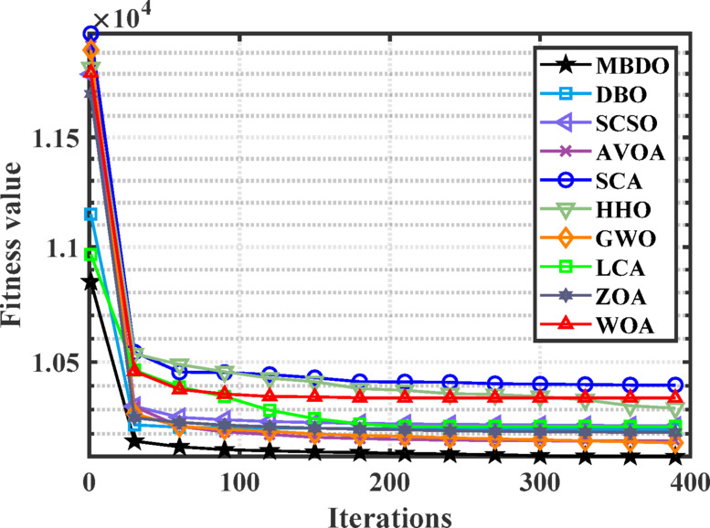 Figure 12
 Figure 13
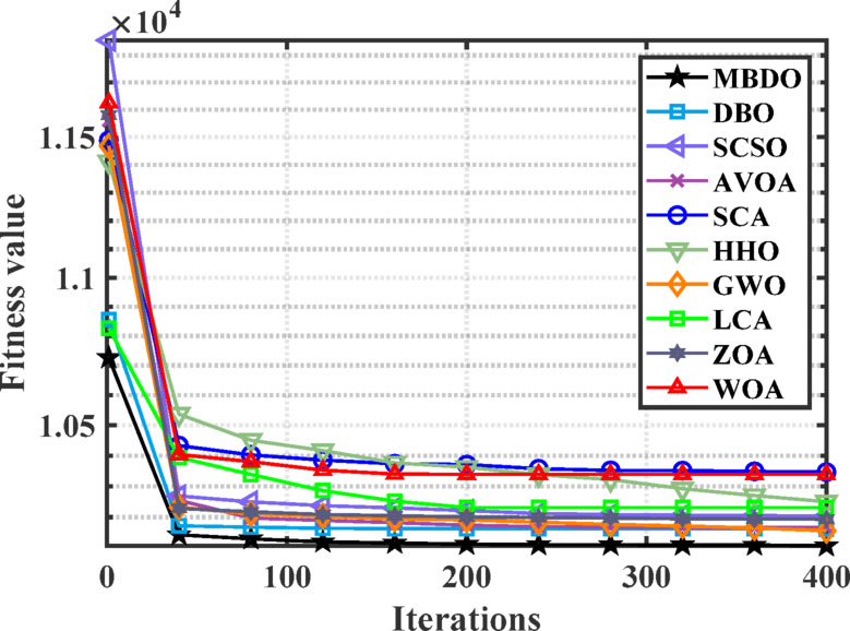 Figure 14
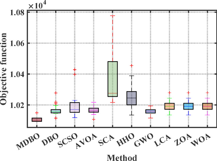 Figure 15
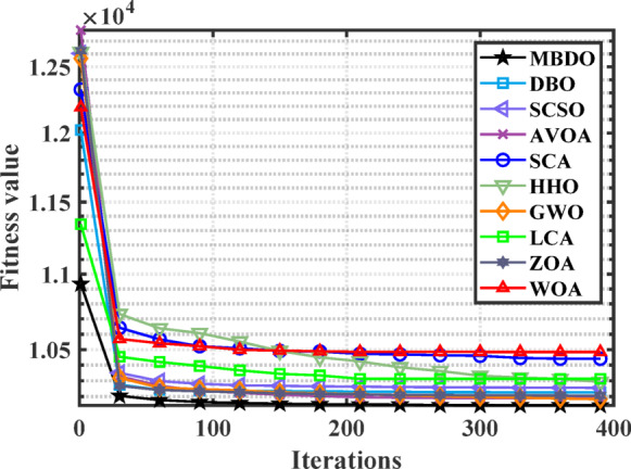 Figure 16
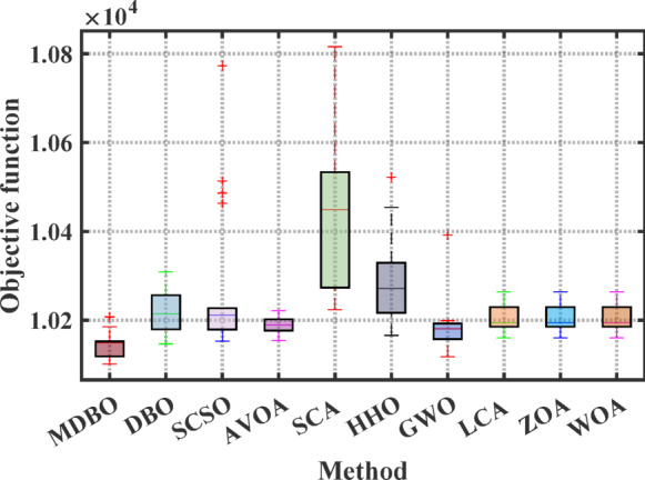 Figure 17
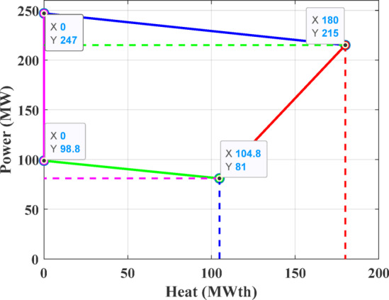 Figure 18
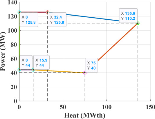 Figure 19
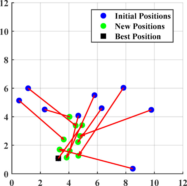 Figure 1
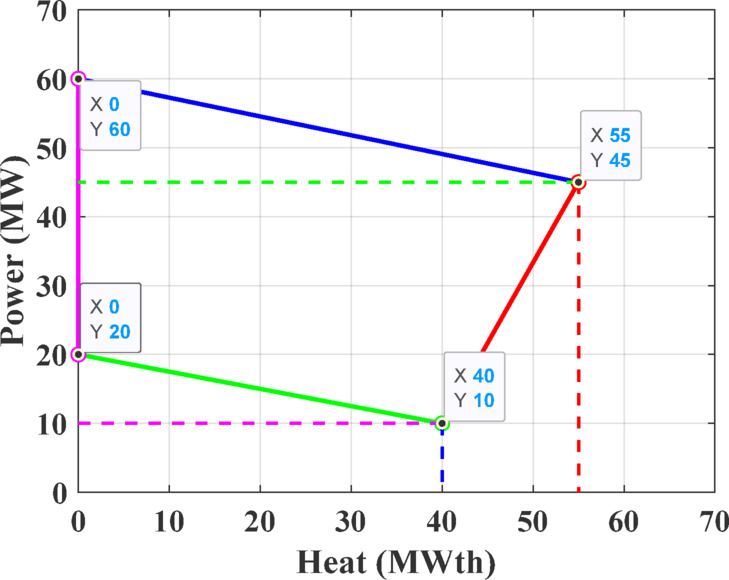 Figure 20
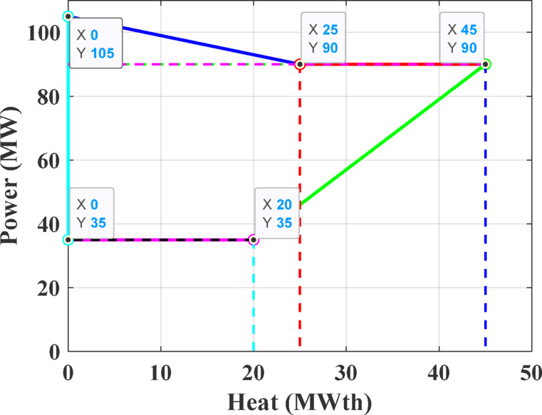 Figure 21
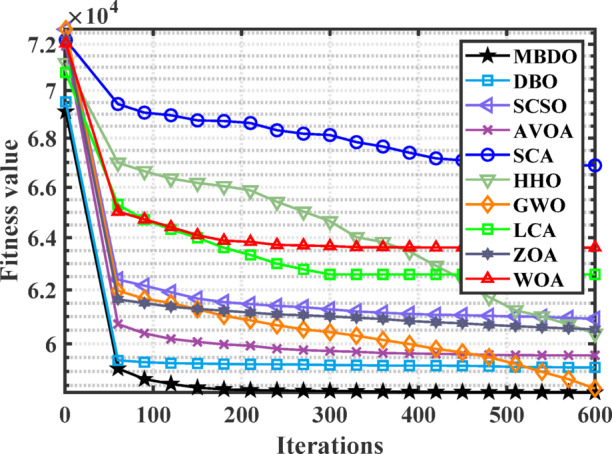 Figure 22
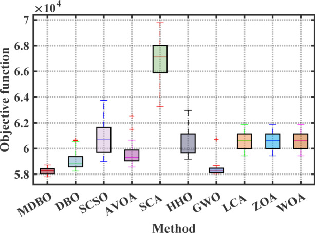 Figure 23
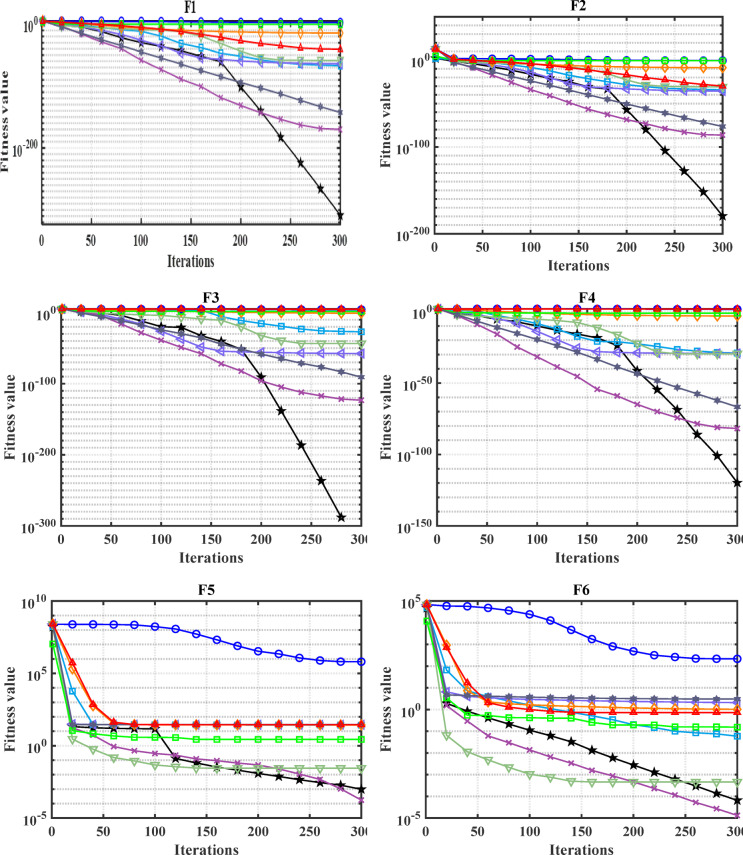 Figure 2
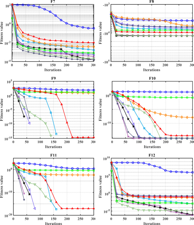 Figure 2
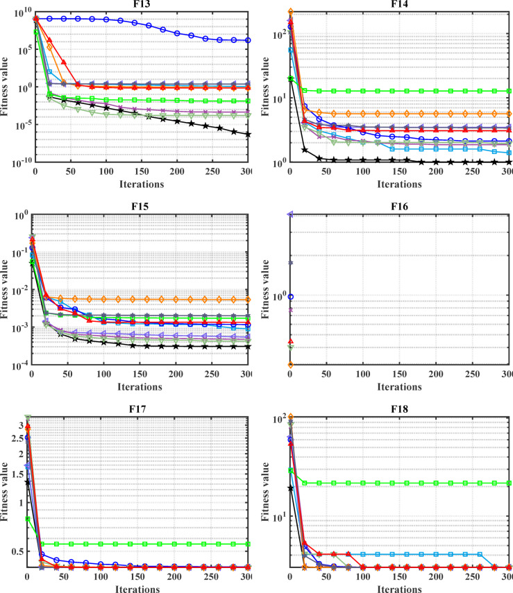 Figure 2
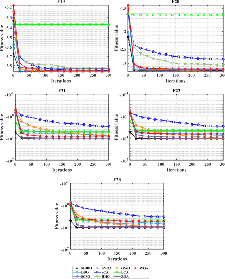 Figure 2
 Figure 3
 Figure 3
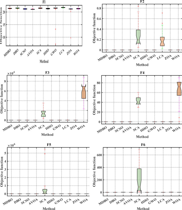 Figure 4
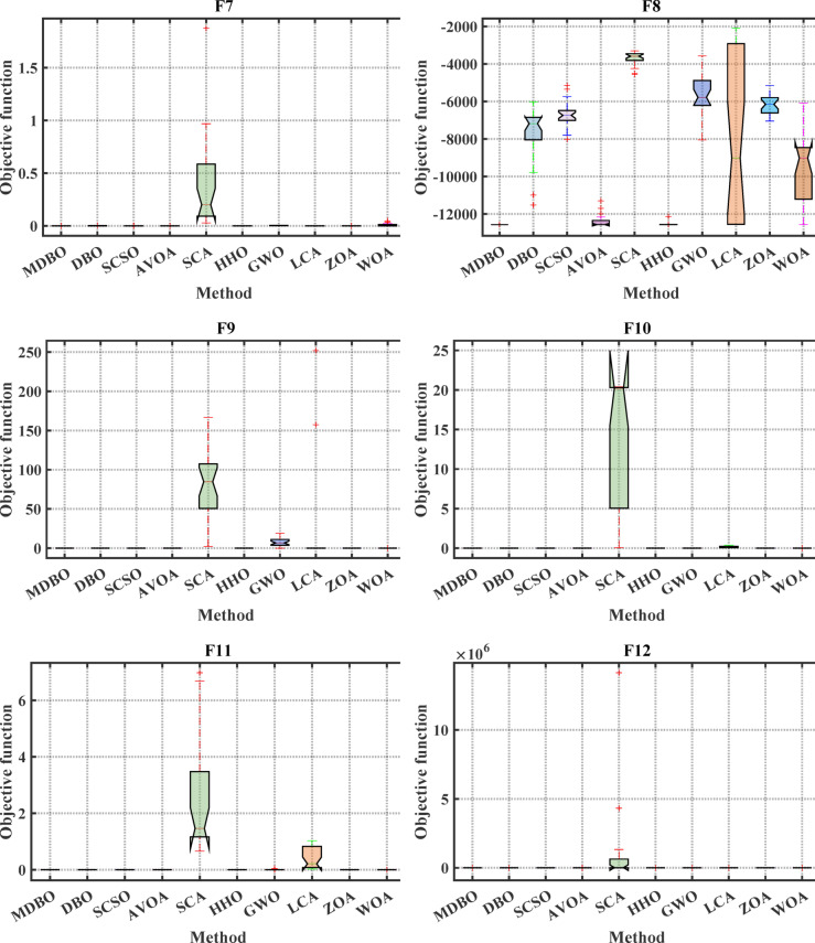 Figure 4
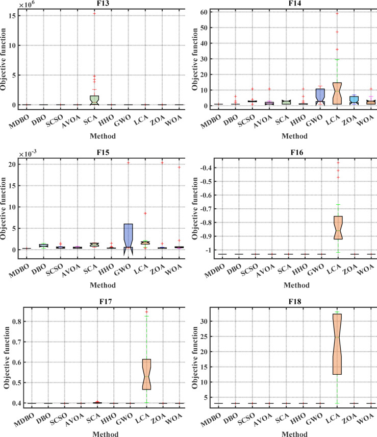 Figure 4
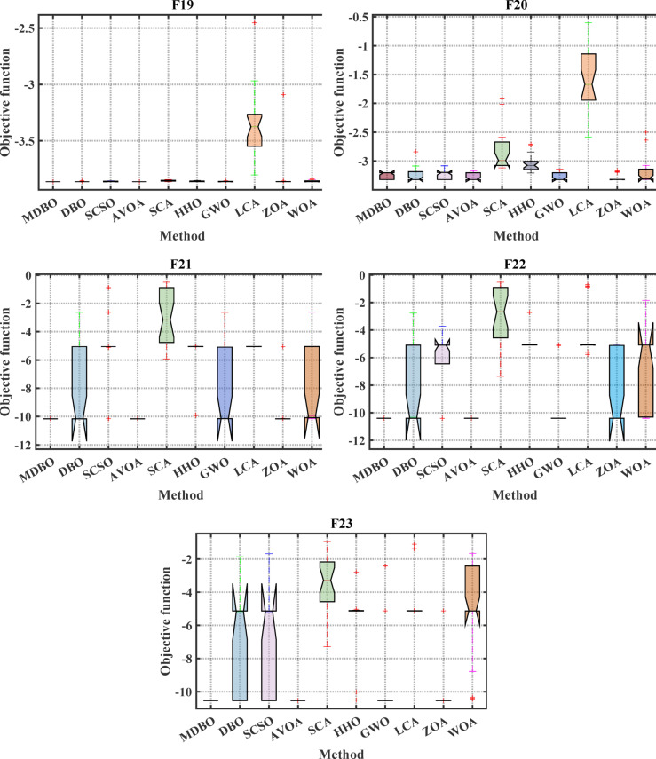 Figure 4
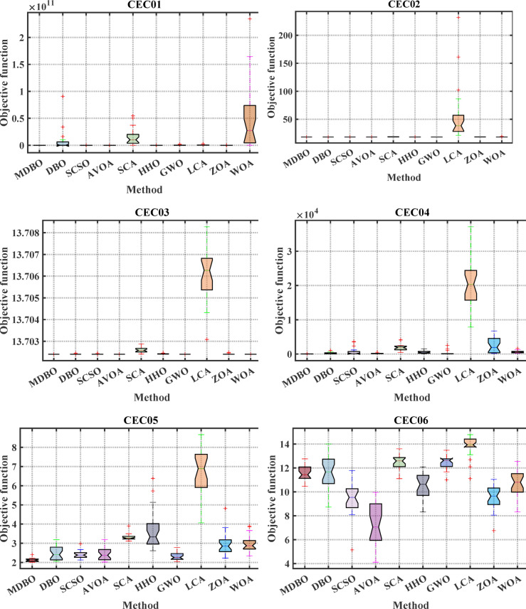 Figure 5
 Figure 5
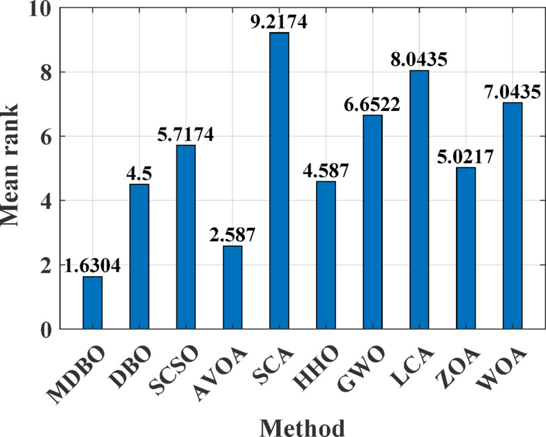 Figure 6
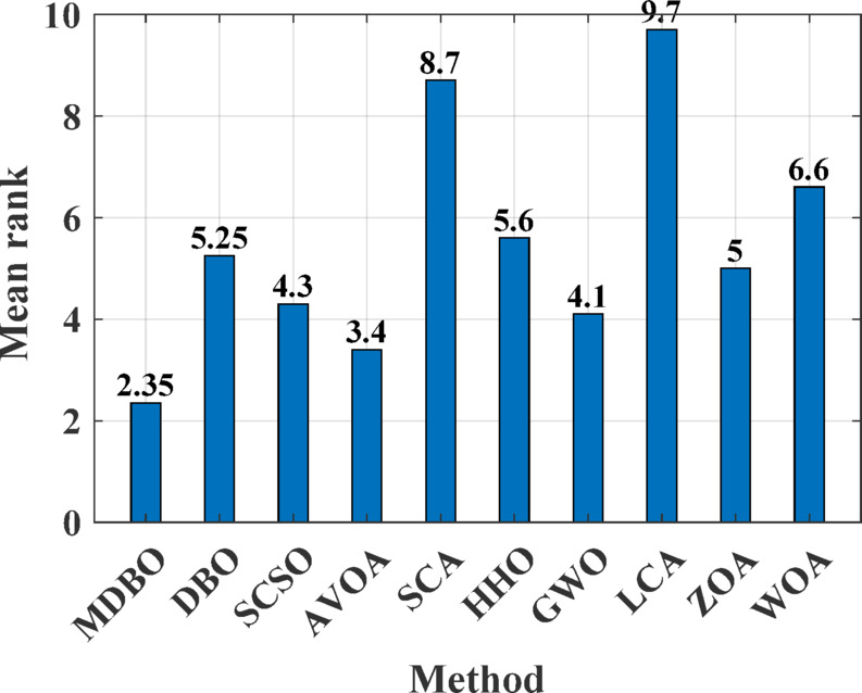 Figure 7
 Figure 8
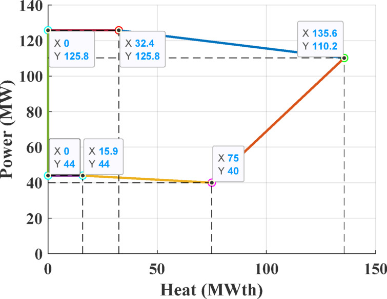 Figure 9
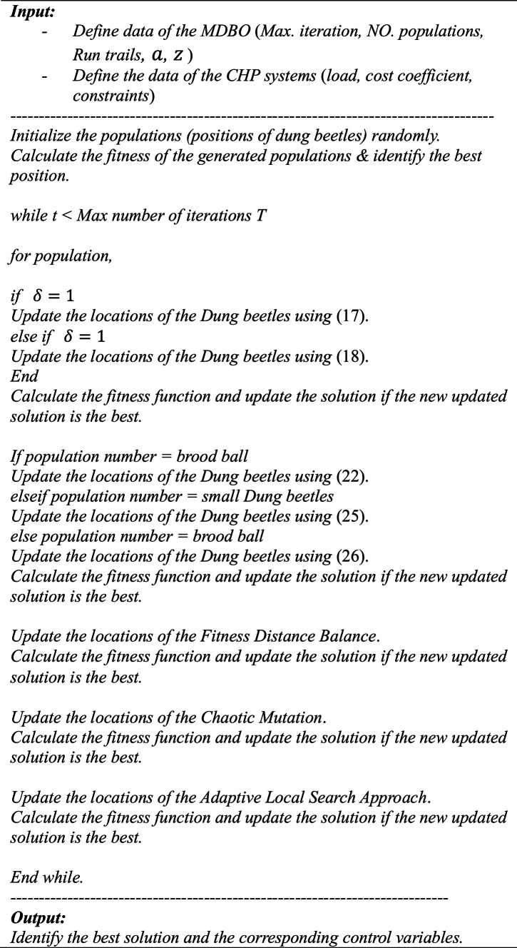 Figure 32
- —Suez Canal University
Peer Reviews
No public reviews on file for this paper yet. If you reviewed it on a platform where reviews are public (OpenReview, ICLR, NeurIPS, ICML), you can paste yours below so the community can read it here.
Videos
No videos yet. Explain this paper in a talk, walkthrough, or lecture? Add one.
Taxonomy
TopicsElectric Power System Optimization · Integrated Energy Systems Optimization · Optimal Power Flow Distribution
Introduction
Background and problem context
Combined Heat and Power (CHP) systems, also known as cogeneration systems, represent a highly efficient and sustainable energy solution applicable across diverse sectors. By producing electrical and thermal energy, CHP systems significantly enhance overall energy utilization and offer substantial environmental advantages. In the context of the global shift toward cleaner and more efficient energy technologies, CHP systems play a pivotal role in reducing greenhouse gas emissions, enhancing energy reliability, and delivering long-term economic benefits. Depending on the technology and its specific application, CHP systems can achieve efficiency levels ranging from 60% to over 80%.
CHP units are consistent with a wide diversity of fuel sources, involving natural gas, biogas, coal, oil, and renewable energy sources such as biomass and solar thermal energy. Unlike conventional power plants that lose a large part of input energy as heat during electricity generation, CHP systems recover and employ this thermal energy to meet heating demands, thereby pushing total system efficiency to nearly 90% ^1,2^. Moreover, CHP systems have the prospect to decrease total fuel costs by 10–40% and lower pollutant emissions by 13–18% ^3^. To completely harness the advantages of CHP systems, it is crucial to address the Combined Heat and Power Economic Dispatch (CHPED) issue, which involves determining the optimum cost-effective schedule for both power and heat generation under various operational constraints ^4^.
Research gap and motivation
Traditional optimization approaches for solving CHPED include the normal boundary intersection method ^5^, branch and bound ^6^, lagrangian approach ^7,8^, sequential quadratic programming ^9^, and benders method ^10,11^. However, these methods often depend heavily on initial conditions, require numerous iterations, and may not consistently converge to the global optimum. Additionally, they can be mathematically complex and computationally intensive.
As a result, heuristic and metaheuristic algorithms have emerged as powerful alternatives for solving CHPED problems. A comprehensive survey of heuristic methods for CHPED is presented in ^12^. Genetic Algorithm (GA)-based approaches have been widely applied to minimize total generation costs while taking into consideration valve-point-loading effects (VPLEs) and transmission power losses (PLs) ^13^. Enhanced GA variants featuring improved crossover and mutation strategies ^14^, as well as the Non-dominated Sorting Genetic Algorithm II (NSGA-II) ^15^, have demonstrated effectiveness in handling mixed-variable scheduling tasks and integrating energy storage systems. Particle Swarm Optimizer (PSO) has been extensively employed for CHPED ^16^, with modifications such as time-varying acceleration coefficients to improve convergence behavior and prevent premature stagnation. VPLEs are often modeled using sinusoidal components added to the cost function. To address uncertainties in demand and renewable energy availability, PSO has been integrated with Monte Carlo simulations ^17^. Additionally, PSO has been utilized to assess dispatch strategies for reducing fuel consumption in coal-fired CHP plants ^18^.
Hybrid algorithms have been proposed to solve the CHPED problem. A hybrid PSO–NSGA-II approach simultaneously optimized both cost and emissions while incorporating transmission PLs ^19^. However, many of these methods have been validated only on small-scale systems (e.g., those comprising 5 to 7 units), limiting their generalizability. The Manta Ray Foraging Optimization (MRFO) has also been implemented to address generation scheduling in systems integrating wind power and VPLEs, achieving cost reductions of up to 8% across both small-scale (5-unit) and large-scale (96-unit) configurations under varying load conditions ^20^. The Cuckoo Search Optimizer (CSO) has emerged as a viable approach for addressing the CHPED issue ^20–23^. Its primary objective is to reduce overall fuel costs while meeting electricity and heat demands, considering constraints such as VPLEs and transmission PLs. In ^21^, CSO was tested on systems of various sizes, including small (5-unit), medium (24-unit), and large (48-unit) configurations. The 5-unit system was evaluated under three distinct heat and power demand scenarios. Similarly, the study in ^22^ demonstrated CSO’s effectiveness across six different test networks with 4, 5, 7, 11, 24, and 48 units. The methodology proposed in ^23^ was applied to five case studies, three involving quadratic cost functions without PLs, and two with non-convex cost functions. Several other metaheuristic approaches have also been employed to solve the CHPED problem, including the grey wolf optimizer (GWO) ^24^, heap-based optimization ^2^, group search optimization ^25^, gravitational search algorithm ^26^, marine predators algorithm ^27^, kho-kho optimization ^28^, a hybrid of weighted vertices-based approach and PSO ^29^. A mixed integer model was proposed to solve the CHPED for 4 units, 5-units, 24-unit, 48-unit, and 96 unit systems ^30^. An improved version of artificial rabbits optimization based on fitness distance balance was presented for solving the CHPED of 4-unit, 5-unit, 7-unit, 24-unit, 48-unit, 96-unit, and 192-unit systems ^31^. The artificial hummingbird algorithm based integrates a linear controlling strategy was developed to solve CHPED for different systems ^32^. An improved version of AVOA based orthogonal oppositional methodology was proposed to solve the CHPED for 48-unit system^33^. A hybrid optimizer based on Harris hawk’s optimizer (HHO), and imperialist competitive algorithm (ICA) was employed to solve the CHPED of 48-unit, 84-unit, and 96-unit systems ^34^.
It is worth mentioning here that metaheuristic optimization algorithms can solve several optimization problems where in a hybrid particle swarm optimizer was presented for optimal coordination of overcurrent relay ^35^ and it can be also applied for optimal placement of electric vehicle stations in distbution grids ^36^. A hybrid simulated annealing (SA) with particle swarm optimization (PSO) was utilized to control variable frequency drives^37^. Artificial intelligence (AI) was proposed for improving the accuracy of objective and physical pressure ratings ^38^. A fast sparse Bayesian learning algorithm was developed for superresolution and the coherent processing of multi-band radar data ^38^. In ^39^, a deep genetic algorithm was suggested for optimizing the channel for signal integrity. In ^40^, a Bayesian posterior loss function technique and a heuristic frequentist approach technique was proposed for to enhance the human decision making.
DBO a robust optimization algorithm that has been applied to solve different optimization problems ^41^. However, several modified versions of DBO were proposed to overcome the stagnation of the traditional DBO to local optima, premature convergence and its low performance where in ^42^, a modified DBO was presented based on Mean Differential Variation and Latin hypercube sampling. A multi-strategy was integrated to DBO based on Levy distribution, two separate cross operators, and Beta distribution to solve path planning problem ^43^. A t-distribution variation approach was applied to enhance the searching ability of the DBO to solve different optimization problems ^44^. Three improvement strategies were integrated to DBO to improve its performance including T-distribution mutation, differential evolutionary variation, cooperative search mechanism and cubic chaotic mapping ^45^. The fractional order calculus methodology was applied with DBO to boost its searching performance in image segmentation ^46^. At the end of this context, the performance of the DBO should be improved for solving large scale problems. Thus, in this paper, three improvement strategies were integrated into DBO to solve the CHPED problem including the fitness distance balance (FDB), Chaotic mutation (CM), and adaptive local search approach (ALSA).
The key contributions
From the previous review, the main associated gap of the applied methods for solving the CHPED is that some papers solved CHPED without considering VPLEs while some papers solved the CHPED with considering PLs only, and some papers solved the CHPED with considering the POZs only. The aim of the papers is to fill the research gap by solving the CHPED of small, medium and large-scale systems considering VPLEs, PLs, and POZs. In addition to that, a modified optimizer is presented to overcome the shortage of traditional DBO via integration of three improvements including ALSA, CM and FDB. Therefore, the contributions to this study can be depicted as follows:
- New Modified Dung Beetle Optimizer (MDBO) is proposed to solve the CHPED based on boosting the exploitation and exploration of the conventional DBO using three strategies including ALSA, CM and FDB.
- MDBO performance has been rigorously assessed using standard benchmark test and CEC-2019 suites to verify its efficiency and robust performance.
- Solving the CHPED problem, considering PLs, VPLE, and POZs for 4 different test systems and the results obtained were compared with other optimization algorithms including SCSA, AVOA, SCA, HHO, GWO, LCA, ZOA, and WOA.
This article is structured as follows: Section "Problem Formulation" outlines the features of CHP units and formulates the economic dispatch problem using DBO and MDBO, considering VPLEs, PLs, and POZs. Section "Methodology" describes the test systems used for validation, followed by optimization outcomes presented in Section "Numerical Results". A comprehensive evaluation of the suggested approach is provided in Section "Conclusions", and the conclusions are summarized in Sect. 6.
Problem formulation
The objective of the CHPED problem is to achieve the lowest possible overall operational cost by optimally coordinating three categories of generation units: those producing only electricity, those generating solely heat, and CHP units. To evaluate different solutions, a fitness function is constructed, taking into account the amount of heat and power generated by each unit. The aggregate operational cost is then determined by summing the individual expenses associated with each type of generation unit, as outlined below:
\documentclass[12pt]{minimal} \usepackage{amsmath} \usepackage{wasysym} \usepackage{amsfonts} \usepackage{amssymb} \usepackage{amsbsy} \usepackage{mathrsfs} \usepackage{upgreek} \setlength{\oddsidemargin}{-69pt} \begin{document}$$Cost_{CHP} = \mathop \sum \limits_{i = 1}^{{N_{p} }} Cost\user2{ }_{i}^{P} \left( {P_{i}^{p} } \right) + \mathop \sum \limits_{j = 1}^{{N_{u} }} Cost\user2{ }_{j}^{H} \left( {H_{j}^{u} } \right) + \mathop \sum \limits_{k = 1}^{{N_{f} }} Cost\user2{ }_{k}^{CHP} \left( {P_{k}^{f} ,H_{k}^{f} } \right)$$\end{document}where, \documentclass[12pt]{minimal} \usepackage{amsmath} \usepackage{wasysym} \usepackage{amsfonts} \usepackage{amssymb} \usepackage{amsbsy} \usepackage{mathrsfs} \usepackage{upgreek} \setlength{\oddsidemargin}{-69pt} \begin{document}$${N}_{p}$$\end{document} refers to the units dedicated solely to electricity generation, \documentclass[12pt]{minimal} \usepackage{amsmath} \usepackage{wasysym} \usepackage{amsfonts} \usepackage{amssymb} \usepackage{amsbsy} \usepackage{mathrsfs} \usepackage{upgreek} \setlength{\oddsidemargin}{-69pt} \begin{document}$${N}_{u}$$\end{document} signifies those units that produce only heat, and \documentclass[12pt]{minimal} \usepackage{amsmath} \usepackage{wasysym} \usepackage{amsfonts} \usepackage{amssymb} \usepackage{amsbsy} \usepackage{mathrsfs} \usepackage{upgreek} \setlength{\oddsidemargin}{-69pt} \begin{document}$${N}_{f}$$\end{document} indicates the CHP units. The cost terms \documentclass[12pt]{minimal} \usepackage{amsmath} \usepackage{wasysym} \usepackage{amsfonts} \usepackage{amssymb} \usepackage{amsbsy} \usepackage{mathrsfs} \usepackage{upgreek} \setlength{\oddsidemargin}{-69pt} \begin{document}$${\text{cost }}_{i}^{P}$$\end{document} , \documentclass[12pt]{minimal} \usepackage{amsmath} \usepackage{wasysym} \usepackage{amsfonts} \usepackage{amssymb} \usepackage{amsbsy} \usepackage{mathrsfs} \usepackage{upgreek} \setlength{\oddsidemargin}{-69pt} \begin{document}$${\text{cost }}_{j}^{H}$$\end{document} , and \documentclass[12pt]{minimal} \usepackage{amsmath} \usepackage{wasysym} \usepackage{amsfonts} \usepackage{amssymb} \usepackage{amsbsy} \usepackage{mathrsfs} \usepackage{upgreek} \setlength{\oddsidemargin}{-69pt} \begin{document}$${\text{cost }}_{k}^{CHP}$$\end{document} represent the cost of generation cost of \documentclass[12pt]{minimal} \usepackage{amsmath} \usepackage{wasysym} \usepackage{amsfonts} \usepackage{amssymb} \usepackage{amsbsy} \usepackage{mathrsfs} \usepackage{upgreek} \setlength{\oddsidemargin}{-69pt} \begin{document}$${i}^{th}$$\end{document} power-only units, the \documentclass[12pt]{minimal} \usepackage{amsmath} \usepackage{wasysym} \usepackage{amsfonts} \usepackage{amssymb} \usepackage{amsbsy} \usepackage{mathrsfs} \usepackage{upgreek} \setlength{\oddsidemargin}{-69pt} \begin{document}$${j}^{th}$$\end{document} heat-only unit, and the \documentclass[12pt]{minimal} \usepackage{amsmath} \usepackage{wasysym} \usepackage{amsfonts} \usepackage{amssymb} \usepackage{amsbsy} \usepackage{mathrsfs} \usepackage{upgreek} \setlength{\oddsidemargin}{-69pt} \begin{document}$${k}^{th}$$\end{document} CHP unit. The cost functions for these units are expressed as follows:
\documentclass[12pt]{minimal} \usepackage{amsmath} \usepackage{wasysym} \usepackage{amsfonts} \usepackage{amssymb} \usepackage{amsbsy} \usepackage{mathrsfs} \usepackage{upgreek} \setlength{\oddsidemargin}{-69pt} \begin{document}$${Cost }_{i}^{P}\left({P}_{i}^{p}\right)={A}_{i}{\left({P}_{i}^{p}\right)}^{2}+{B}_{i}{P}_{i}^{p}+{Q}_{i}+\left|{T}_{i}\mathrm{sin}\left({G}_{i}\left({P}_{i}^{p,Min}-{P}_{i}^{p}\right)\right)\right|$$\end{document} \documentclass[12pt]{minimal} \usepackage{amsmath} \usepackage{wasysym} \usepackage{amsfonts} \usepackage{amssymb} \usepackage{amsbsy} \usepackage{mathrsfs} \usepackage{upgreek} \setlength{\oddsidemargin}{-69pt} \begin{document}$${Cost }_{j}^{H}\left({H}_{j}^{u}\right)={A}_{j}{\left({H}_{j}^{u}\right)}^{2}+{B}_{j}{H}_{j}^{u}+{Q}_{j}$$\end{document} \documentclass[12pt]{minimal} \usepackage{amsmath} \usepackage{wasysym} \usepackage{amsfonts} \usepackage{amssymb} \usepackage{amsbsy} \usepackage{mathrsfs} \usepackage{upgreek} \setlength{\oddsidemargin}{-69pt} \begin{document}$${Cost }_{k}^{CHP}\left({P}_{k}^{f},{H}_{k}^{f}\right)={A}_{k}{\left({P}_{k}^{f}\right)}^{2}+{B}_{k}{P}_{k}^{f}+{Q}_{k}+{T}_{k}{\left({H}_{k}^{f}\right)}^{2}+{G}_{k}{H}_{k}^{f}+{V}_{k}{P}_{k}^{f}{H}_{k}^{f}$$\end{document}- For power-only units, cost was modeled using coefficients \documentclass[12pt]{minimal} \usepackage{amsmath} \usepackage{wasysym} \usepackage{amsfonts} \usepackage{amssymb} \usepackage{amsbsy} \usepackage{mathrsfs} \usepackage{upgreek} \setlength{\oddsidemargin}{-69pt} \begin{document}$${A}_{i}, {B}_{i}$$\end{document} , \documentclass[12pt]{minimal} \usepackage{amsmath} \usepackage{wasysym} \usepackage{amsfonts} \usepackage{amssymb} \usepackage{amsbsy} \usepackage{mathrsfs} \usepackage{upgreek} \setlength{\oddsidemargin}{-69pt} \begin{document}$${Q}_{i}, {T}_{i},$$\end{document} and \documentclass[12pt]{minimal} \usepackage{amsmath} \usepackage{wasysym} \usepackage{amsfonts} \usepackage{amssymb} \usepackage{amsbsy} \usepackage{mathrsfs} \usepackage{upgreek} \setlength{\oddsidemargin}{-69pt} \begin{document}$${G}_{i}$$\end{document} , representing the cost parameters for \documentclass[12pt]{minimal} \usepackage{amsmath} \usepackage{wasysym} \usepackage{amsfonts} \usepackage{amssymb} \usepackage{amsbsy} \usepackage{mathrsfs} \usepackage{upgreek} \setlength{\oddsidemargin}{-69pt} \begin{document}$${i}^{th}$$\end{document} electricity production units.
- For heat-only units, cost was modeled using coefficients \documentclass[12pt]{minimal} \usepackage{amsmath} \usepackage{wasysym} \usepackage{amsfonts} \usepackage{amssymb} \usepackage{amsbsy} \usepackage{mathrsfs} \usepackage{upgreek} \setlength{\oddsidemargin}{-69pt} \begin{document}$${A}_{j}, {B}_{j}$$\end{document} , and \documentclass[12pt]{minimal} \usepackage{amsmath} \usepackage{wasysym} \usepackage{amsfonts} \usepackage{amssymb} \usepackage{amsbsy} \usepackage{mathrsfs} \usepackage{upgreek} \setlength{\oddsidemargin}{-69pt} \begin{document}$${Q}_{j}$$\end{document} , which account for the heat generation expenses.
- For CHP units, cost was represented using coefficients \documentclass[12pt]{minimal} \usepackage{amsmath} \usepackage{wasysym} \usepackage{amsfonts} \usepackage{amssymb} \usepackage{amsbsy} \usepackage{mathrsfs} \usepackage{upgreek} \setlength{\oddsidemargin}{-69pt} \begin{document}$${A}_{k}, {B}_{k}{, Q}_{k}, {T}_{k}, {G}_{k}$$\end{document} , and \documentclass[12pt]{minimal} \usepackage{amsmath} \usepackage{wasysym} \usepackage{amsfonts} \usepackage{amssymb} \usepackage{amsbsy} \usepackage{mathrsfs} \usepackage{upgreek} \setlength{\oddsidemargin}{-69pt} \begin{document}$${V}_{k}$$\end{document} , which captures the combined cost of electricity and heat production for the \documentclass[12pt]{minimal} \usepackage{amsmath} \usepackage{wasysym} \usepackage{amsfonts} \usepackage{amssymb} \usepackage{amsbsy} \usepackage{mathrsfs} \usepackage{upgreek} \setlength{\oddsidemargin}{-69pt} \begin{document}$${k}^{th}$$\end{document} units ^47^.
Constraints in the CHPED problem
The CHPED problem formulation includes both equality and inequality constraints to ensure energy balance and adherence to operational limits:
Equality constraints
The equality constraints include the power balanced with and without power losses asdescribed in Eqs. (5) and (6), as well as the heat balanced of hsystem as decribed in (7). In addation to that the equality constraints include the capacities of only-power units, heat-only units and the CHP units as depicted in (8), (9), and (10), respectivly. Furthermore, the prohibted zones of the generation units are described in (11).
\documentclass[12pt]{minimal} \usepackage{amsmath} \usepackage{wasysym} \usepackage{amsfonts} \usepackage{amssymb} \usepackage{amsbsy} \usepackage{mathrsfs} \usepackage{upgreek} \setlength{\oddsidemargin}{-69pt} \begin{document}$$\mathop \sum \limits_{i = 1}^{{N_{p} }} P_{i}^{p} + \mathop \sum \limits_{k = 1}^{{N_{f} }} P_{k}^{f} - P_{{\text{demand }}} = 0$$\end{document} \documentclass[12pt]{minimal} \usepackage{amsmath} \usepackage{wasysym} \usepackage{amsfonts} \usepackage{amssymb} \usepackage{amsbsy} \usepackage{mathrsfs} \usepackage{upgreek} \setlength{\oddsidemargin}{-69pt} \begin{document}$$\mathop \sum \limits_{i = 1}^{{N_{p} }} P_{i}^{p} + \mathop \sum \limits_{k = 1}^{{N_{f} }} P_{k}^{N} - P_{{\text{demand }}} - P_{{\text{losses }}} = 0$$\end{document}where; Plosses is power losses, while Pdemand is the power demand.
\documentclass[12pt]{minimal} \usepackage{amsmath} \usepackage{wasysym} \usepackage{amsfonts} \usepackage{amssymb} \usepackage{amsbsy} \usepackage{mathrsfs} \usepackage{upgreek} \setlength{\oddsidemargin}{-69pt} \begin{document}$$\mathop \sum \limits_{k = 1}^{{N_{f} }} H_{k}^{f} + \mathop \sum \limits_{j = 1}^{{N_{u} }} H_{j}^{u} - H_{{\text{demand }}} = 0$$\end{document} \documentclass[12pt]{minimal} \usepackage{amsmath} \usepackage{wasysym} \usepackage{amsfonts} \usepackage{amssymb} \usepackage{amsbsy} \usepackage{mathrsfs} \usepackage{upgreek} \setlength{\oddsidemargin}{-69pt} \begin{document}$$P_{power\_only} = \mathop \sum \limits_{i = 1}^{{N_{p} }} \left[ {Max\left( {P_{i}^{p} - P_{i}^{pMax} ,0} \right) + Max\left( {P_{i}^{pMin} - P_{i}^{p} ,0} \right)} \right]$$\end{document} \documentclass[12pt]{minimal} \usepackage{amsmath} \usepackage{wasysym} \usepackage{amsfonts} \usepackage{amssymb} \usepackage{amsbsy} \usepackage{mathrsfs} \usepackage{upgreek} \setlength{\oddsidemargin}{-69pt} \begin{document}$$P_{heat\_only} = \mathop \sum \limits_{j = 1}^{{N_{u} }} \left[ {Max\left( {H_{j}^{u} - H_{j}^{u, Max } ,0} \right) + Max\left( {H_{j}^{u,Min} - H_{j}^{u} ,0} \right)} \right]$$\end{document} \documentclass[12pt]{minimal} \usepackage{amsmath} \usepackage{wasysym} \usepackage{amsfonts} \usepackage{amssymb} \usepackage{amsbsy} \usepackage{mathrsfs} \usepackage{upgreek} \setlength{\oddsidemargin}{-69pt} \begin{document}$$P_{CHP} = \mathop \sum \limits_{k - 1}^{{N_{f} }} \left[ {\begin{array}{*{20}c} {Max\left( {P_{k}^{f} - P_{k}^{f,Max} \left( {H_{k}^{f} } \right),0} \right) + Max\left( {P_{k}^{f,Min} \left( {H_{k}^{f} } \right) - P_{k}^{f} ,0} \right) + } \\ {Max\left( {H_{k}^{f} - H_{k}^{f,Max} \left( {P_{k}^{f} } \right),0} \right) + Max\left( {H_{k}^{fMin} \left( {P_{k}^{f} } \right) - H_{k}^{f} ,0} \right)} \\ \end{array} } \right]$$\end{document} \documentclass[12pt]{minimal} \usepackage{amsmath} \usepackage{wasysym} \usepackage{amsfonts} \usepackage{amssymb} \usepackage{amsbsy} \usepackage{mathrsfs} \usepackage{upgreek} \setlength{\oddsidemargin}{-69pt} \begin{document}$$P_{{POz_{s} }} = \mathop \sum \limits_{i = 1}^{{N_{p} }} \left[ {\xi_{i} \mathop \sum \limits_{V = 1}^{{Z_{i} }} Min\left( {Max\left( {P_{i}^{p} - P_{i,V}^{L} ,0} \right),Max\left( {P_{i,V}^{U} - P_{i}^{p} ,\;0} \right)} \right)} \right]$$\end{document}The inequality constraints
Each power-only unit must operate within its designated generation limits. These constraints ensure that the power output from the \documentclass[12pt]{minimal} \usepackage{amsmath} \usepackage{wasysym} \usepackage{amsfonts} \usepackage{amssymb} \usepackage{amsbsy} \usepackage{mathrsfs} \usepackage{upgreek} \setlength{\oddsidemargin}{-69pt} \begin{document}$${i}^{th}$$\end{document} unit stays within the allowable lower and upper bounds.
\documentclass[12pt]{minimal} \usepackage{amsmath} \usepackage{wasysym} \usepackage{amsfonts} \usepackage{amssymb} \usepackage{amsbsy} \usepackage{mathrsfs} \usepackage{upgreek} \setlength{\oddsidemargin}{-69pt} \begin{document}$$P_{{i{\mathrm{,Min}}}}^{{power\_only_{ } }} \le P_{i}^{power\_only} \le P_{i,Max}^{{power\_only_{ } }} i = 1, \ldots ,N_{p}$$\end{document}The heat output from each heat-only unit is restricted by its minimum and maximum generation capabilities.
\documentclass[12pt]{minimal} \usepackage{amsmath} \usepackage{wasysym} \usepackage{amsfonts} \usepackage{amssymb} \usepackage{amsbsy} \usepackage{mathrsfs} \usepackage{upgreek} \setlength{\oddsidemargin}{-69pt} \begin{document}$$\left({H}_{j}^{f}\right)\le {H}_{j}^{f}\le \left({H}_{j}^{f}\right)j, {\forall }_{j}$$\end{document}where \documentclass[12pt]{minimal} \usepackage{amsmath} \usepackage{wasysym} \usepackage{amsfonts} \usepackage{amssymb} \usepackage{amsbsy} \usepackage{mathrsfs} \usepackage{upgreek} \setlength{\oddsidemargin}{-69pt} \begin{document}$${H}_{j}^{{f}_{Max}}$$\end{document} and \documentclass[12pt]{minimal} \usepackage{amsmath} \usepackage{wasysym} \usepackage{amsfonts} \usepackage{amssymb} \usepackage{amsbsy} \usepackage{mathrsfs} \usepackage{upgreek} \setlength{\oddsidemargin}{-69pt} \begin{document}$${H}_{j}^{{f}_{Min}}$$\end{document} represent the upper and lower restrictions of heat output from the \documentclass[12pt]{minimal} \usepackage{amsmath} \usepackage{wasysym} \usepackage{amsfonts} \usepackage{amssymb} \usepackage{amsbsy} \usepackage{mathrsfs} \usepackage{upgreek} \setlength{\oddsidemargin}{-69pt} \begin{document}$${j}^{th}$$\end{document} unit, correspondingly.
The CHP units concurrently generate both heat and power, are also subject to operational limits.
\documentclass[12pt]{minimal} \usepackage{amsmath} \usepackage{wasysym} \usepackage{amsfonts} \usepackage{amssymb} \usepackage{amsbsy} \usepackage{mathrsfs} \usepackage{upgreek} \setlength{\oddsidemargin}{-69pt} \begin{document}$${H}_{j}^{{f}_{Min}}\left({P}_{j}^{f}\right)\le {H}_{j}^{f}\le {H}_{j}^{{f}_{Max}}\left({P}_{j}^{f}\right)j=1,\dots ,{N}_{f}$$\end{document} \documentclass[12pt]{minimal} \usepackage{amsmath} \usepackage{wasysym} \usepackage{amsfonts} \usepackage{amssymb} \usepackage{amsbsy} \usepackage{mathrsfs} \usepackage{upgreek} \setlength{\oddsidemargin}{-69pt} \begin{document}$${H}_{k}^{{u}_{Min}}\le {H}_{k}^{u}\le {H}_{k}^{{u}_{Max}}k=1,\dots ,{N}_{u}$$\end{document}The electrical power generation from the \documentclass[12pt]{minimal} \usepackage{amsmath} \usepackage{wasysym} \usepackage{amsfonts} \usepackage{amssymb} \usepackage{amsbsy} \usepackage{mathrsfs} \usepackage{upgreek} \setlength{\oddsidemargin}{-69pt} \begin{document}$${k}^{th}$$\end{document} CHP unit must lie within the bounds \documentclass[12pt]{minimal} \usepackage{amsmath} \usepackage{wasysym} \usepackage{amsfonts} \usepackage{amssymb} \usepackage{amsbsy} \usepackage{mathrsfs} \usepackage{upgreek} \setlength{\oddsidemargin}{-69pt} \begin{document}$${P}_{j}^{{f}_{\text{Max }}}$$\end{document} and \documentclass[12pt]{minimal} \usepackage{amsmath} \usepackage{wasysym} \usepackage{amsfonts} \usepackage{amssymb} \usepackage{amsbsy} \usepackage{mathrsfs} \usepackage{upgreek} \setlength{\oddsidemargin}{-69pt} \begin{document}$${P}_{j}^{{f}_{\text{Min }}}{H}_{k}^{f}$$\end{document} , which denote the lower and upper bounds of the power output capacity for the respective unit, respectively. Likewise, the heat output from the same CHP unit must fall within the limits \documentclass[12pt]{minimal} \usepackage{amsmath} \usepackage{wasysym} \usepackage{amsfonts} \usepackage{amssymb} \usepackage{amsbsy} \usepackage{mathrsfs} \usepackage{upgreek} \setlength{\oddsidemargin}{-69pt} \begin{document}$${H}_{j}^{{f}_{Min}} {P}_{k}^{f}$$\end{document} \documentclass[12pt]{minimal} \usepackage{amsmath} \usepackage{wasysym} \usepackage{amsfonts} \usepackage{amssymb} \usepackage{amsbsy} \usepackage{mathrsfs} \usepackage{upgreek} \setlength{\oddsidemargin}{-69pt} \begin{document}$${H}_{j}^{{f}_{Max}} {P}_{k}^{c}$$\end{document} , which denote the minimum and maximum allowable heat generation from the \documentclass[12pt]{minimal} \usepackage{amsmath} \usepackage{wasysym} \usepackage{amsfonts} \usepackage{amssymb} \usepackage{amsbsy} \usepackage{mathrsfs} \usepackage{upgreek} \setlength{\oddsidemargin}{-69pt} \begin{document}$${k}^{th}$$\end{document} CHP unit, respectively.Also, Certain regions within the power generation range are deemed infeasible due to operational constraints or safety considerations; these segments are referred to as POZs. The feasible power output range for the \documentclass[12pt]{minimal} \usepackage{amsmath} \usepackage{wasysym} \usepackage{amsfonts} \usepackage{amssymb} \usepackage{amsbsy} \usepackage{mathrsfs} \usepackage{upgreek} \setlength{\oddsidemargin}{-69pt} \begin{document}$${i}^{th}$$\end{document} power-only unit is characterized in accordance with Eq. (16). Here, \documentclass[12pt]{minimal} \usepackage{amsmath} \usepackage{wasysym} \usepackage{amsfonts} \usepackage{amssymb} \usepackage{amsbsy} \usepackage{mathrsfs} \usepackage{upgreek} \setlength{\oddsidemargin}{-69pt} \begin{document}$${P}_{i}^{n,L}$$\end{document} and \documentclass[12pt]{minimal} \usepackage{amsmath} \usepackage{wasysym} \usepackage{amsfonts} \usepackage{amssymb} \usepackage{amsbsy} \usepackage{mathrsfs} \usepackage{upgreek} \setlength{\oddsidemargin}{-69pt} \begin{document}$${P}_{i}^{n,U}$$\end{document} represent the lower and upper limits of the \documentclass[12pt]{minimal} \usepackage{amsmath} \usepackage{wasysym} \usepackage{amsfonts} \usepackage{amssymb} \usepackage{amsbsy} \usepackage{mathrsfs} \usepackage{upgreek} \setlength{\oddsidemargin}{-69pt} \begin{document}$${n}^{th}$$\end{document} POZ for the \documentclass[12pt]{minimal} \usepackage{amsmath} \usepackage{wasysym} \usepackage{amsfonts} \usepackage{amssymb} \usepackage{amsbsy} \usepackage{mathrsfs} \usepackage{upgreek} \setlength{\oddsidemargin}{-69pt} \begin{document}$${i}^{th}$$\end{document} power-only unit, respectively, while \documentclass[12pt]{minimal} \usepackage{amsmath} \usepackage{wasysym} \usepackage{amsfonts} \usepackage{amssymb} \usepackage{amsbsy} \usepackage{mathrsfs} \usepackage{upgreek} \setlength{\oddsidemargin}{-69pt} \begin{document}$${Z}_{i}$$\end{document} denotes the total count of such POZs associated with the unit.
\documentclass[12pt]{minimal} \usepackage{amsmath} \usepackage{wasysym} \usepackage{amsfonts} \usepackage{amssymb} \usepackage{amsbsy} \usepackage{mathrsfs} \usepackage{upgreek} \setlength{\oddsidemargin}{-69pt} \begin{document}$$\left\{\begin{array}{c}{P}_{i}^{\text{ Min }}\le {P}_{i}^{power\_only}\le {P}_{i}^{Max}\\ {P}_{i}^{n,l}\le {P}_{i}^{powe{r}_{only}}\le {P}_{i}^{n,U}, {\forall }_{n} \in \left[\mathrm{1,2},\dots ,{Z}_{i}\right]\\ {P}_{i}^{{Z}_{1},U}\le {P}_{i}^{p}\le {P}_{i}^{p,Max}\end{array}\right.$$\end{document}Methodology
Dung beetle optimization (DBO)
The Dung Beetle Optimization (DBO) algorithm is a biologically inspired based metaheuristic that simulates the unique behaviors of the dung beetles. It incorporates four key activities: Rolling, Spawning, Foraging, and Stealing, which collectively guide the population of virtual dung beetles searching for optimal solutions.
Rollerball Dung Beetle (rolling)
Dung beetles roll dung balls in straight paths while navigating using sunlight. This behavior is modeled in DBO for updating the beetle’s position using Eq. (22) ^41^:
\documentclass[12pt]{minimal} \usepackage{amsmath} \usepackage{wasysym} \usepackage{amsfonts} \usepackage{amssymb} \usepackage{amsbsy} \usepackage{mathrsfs} \usepackage{upgreek} \setlength{\oddsidemargin}{-69pt} \begin{document}$$\begin{array}{c}{x}_{i}(tt+1)={x}_{i}(tt)+\alpha \cdot k\cdot {x}_{i}(tt-1)+b\cdot \Delta x\\ \Delta x=\left|{x}_{i}(tt)-{X}^{w}\right|\end{array}$$\end{document}where: \documentclass[12pt]{minimal} \usepackage{amsmath} \usepackage{wasysym} \usepackage{amsfonts} \usepackage{amssymb} \usepackage{amsbsy} \usepackage{mathrsfs} \usepackage{upgreek} \setlength{\oddsidemargin}{-69pt} \begin{document}$${x}_{i}(tt)$$\end{document} is the position of the i^th^ beetle at time \documentclass[12pt]{minimal} \usepackage{amsmath} \usepackage{wasysym} \usepackage{amsfonts} \usepackage{amssymb} \usepackage{amsbsy} \usepackage{mathrsfs} \usepackage{upgreek} \setlength{\oddsidemargin}{-69pt} \begin{document}$$(tt)$$\end{document} . \documentclass[12pt]{minimal} \usepackage{amsmath} \usepackage{wasysym} \usepackage{amsfonts} \usepackage{amssymb} \usepackage{amsbsy} \usepackage{mathrsfs} \usepackage{upgreek} \setlength{\oddsidemargin}{-69pt} \begin{document}$$\alpha$$\end{document} determines if the beetle deviates from its original path (random directional factor, randomly set to 1 or -1). \documentclass[12pt]{minimal} \usepackage{amsmath} \usepackage{wasysym} \usepackage{amsfonts} \usepackage{amssymb} \usepackage{amsbsy} \usepackage{mathrsfs} \usepackage{upgreek} \setlength{\oddsidemargin}{-69pt} \begin{document}$$k$$\end{document} is a deflection coefficient (between 0 and 0.2). \documentclass[12pt]{minimal} \usepackage{amsmath} \usepackage{wasysym} \usepackage{amsfonts} \usepackage{amssymb} \usepackage{amsbsy} \usepackage{mathrsfs} \usepackage{upgreek} \setlength{\oddsidemargin}{-69pt} \begin{document}$$b$$\end{document} is a constant in the range [0, 1]. \documentclass[12pt]{minimal} \usepackage{amsmath} \usepackage{wasysym} \usepackage{amsfonts} \usepackage{amssymb} \usepackage{amsbsy} \usepackage{mathrsfs} \usepackage{upgreek} \setlength{\oddsidemargin}{-69pt} \begin{document}$$\Delta x$$\end{document} simulates the beetle’s displacement toward the light source. If the beetle encounters an obstacle, it simulates directional change via a dancing behavior, modifying its position based on Eq. (23).
\documentclass[12pt]{minimal} \usepackage{amsmath} \usepackage{wasysym} \usepackage{amsfonts} \usepackage{amssymb} \usepackage{amsbsy} \usepackage{mathrsfs} \usepackage{upgreek} \setlength{\oddsidemargin}{-69pt} \begin{document}$${x}_{i}(tt+1)={x}_{i}(tt)+\mathrm{tan}(\theta )\left|{x}_{i}(tt)-{x}_{i}(tt-1)\right|$$\end{document}The angle *θ ⊆ [0, *π] determines direction adjustment, with no update occurring when θ = 0, π ∕ 2, and π.
Spawning behavior
Dung beetles choose safe zones for laying eggs. DBO models this through adaptive boundaries for local exploration:
\documentclass[12pt]{minimal} \usepackage{amsmath} \usepackage{wasysym} \usepackage{amsfonts} \usepackage{amssymb} \usepackage{amsbsy} \usepackage{mathrsfs} \usepackage{upgreek} \setlength{\oddsidemargin}{-69pt} \begin{document}$$L{b}^{*}=max\left({X}^{*}\times (1-R),Lb\right)$$\end{document} \documentclass[12pt]{minimal} \usepackage{amsmath} \usepackage{wasysym} \usepackage{amsfonts} \usepackage{amssymb} \usepackage{amsbsy} \usepackage{mathrsfs} \usepackage{upgreek} \setlength{\oddsidemargin}{-69pt} \begin{document}$$U{b}^{*}=min\left({X}^{*}\times (1+R),Ub\right)$$\end{document} \documentclass[12pt]{minimal} \usepackage{amsmath} \usepackage{wasysym} \usepackage{amsfonts} \usepackage{amssymb} \usepackage{amsbsy} \usepackage{mathrsfs} \usepackage{upgreek} \setlength{\oddsidemargin}{-69pt} \begin{document}$$R=1-\frac{t}{{T}_{max}}$$\end{document}where, \documentclass[12pt]{minimal} \usepackage{amsmath} \usepackage{wasysym} \usepackage{amsfonts} \usepackage{amssymb} \usepackage{amsbsy} \usepackage{mathrsfs} \usepackage{upgreek} \setlength{\oddsidemargin}{-69pt} \begin{document}$$L{b}^{*}$$\end{document} and \documentclass[12pt]{minimal} \usepackage{amsmath} \usepackage{wasysym} \usepackage{amsfonts} \usepackage{amssymb} \usepackage{amsbsy} \usepackage{mathrsfs} \usepackage{upgreek} \setlength{\oddsidemargin}{-69pt} \begin{document}$$U{b}^{*}$$\end{document} is the lower and upper constraints of the spawning region, \documentclass[12pt]{minimal} \usepackage{amsmath} \usepackage{wasysym} \usepackage{amsfonts} \usepackage{amssymb} \usepackage{amsbsy} \usepackage{mathrsfs} \usepackage{upgreek} \setlength{\oddsidemargin}{-69pt} \begin{document}$$Lb$$\end{document} and \documentclass[12pt]{minimal} \usepackage{amsmath} \usepackage{wasysym} \usepackage{amsfonts} \usepackage{amssymb} \usepackage{amsbsy} \usepackage{mathrsfs} \usepackage{upgreek} \setlength{\oddsidemargin}{-69pt} \begin{document}$$Ub$$\end{document} is the Original lower and upper constraints, \documentclass[12pt]{minimal} \usepackage{amsmath} \usepackage{wasysym} \usepackage{amsfonts} \usepackage{amssymb} \usepackage{amsbsy} \usepackage{mathrsfs} \usepackage{upgreek} \setlength{\oddsidemargin}{-69pt} \begin{document}$${X}^{*}$$\end{document} is the current best solution, \documentclass[12pt]{minimal} \usepackage{amsmath} \usepackage{wasysym} \usepackage{amsfonts} \usepackage{amssymb} \usepackage{amsbsy} \usepackage{mathrsfs} \usepackage{upgreek} \setlength{\oddsidemargin}{-69pt} \begin{document}$$R$$\end{document} is the decay factor over iterations, while \documentclass[12pt]{minimal} \usepackage{amsmath} \usepackage{wasysym} \usepackage{amsfonts} \usepackage{amssymb} \usepackage{amsbsy} \usepackage{mathrsfs} \usepackage{upgreek} \setlength{\oddsidemargin}{-69pt} \begin{document}$${T}_{max}$$\end{document} is the maximum number of iterations.
The position update in spawning is defined by Eq. (22), using random values \documentclass[12pt]{minimal} \usepackage{amsmath} \usepackage{wasysym} \usepackage{amsfonts} \usepackage{amssymb} \usepackage{amsbsy} \usepackage{mathrsfs} \usepackage{upgreek} \setlength{\oddsidemargin}{-69pt} \begin{document}$$b1$$\end{document} and \documentclass[12pt]{minimal} \usepackage{amsmath} \usepackage{wasysym} \usepackage{amsfonts} \usepackage{amssymb} \usepackage{amsbsy} \usepackage{mathrsfs} \usepackage{upgreek} \setlength{\oddsidemargin}{-69pt} \begin{document}$$b2$$\end{document} .
\documentclass[12pt]{minimal} \usepackage{amsmath} \usepackage{wasysym} \usepackage{amsfonts} \usepackage{amssymb} \usepackage{amsbsy} \usepackage{mathrsfs} \usepackage{upgreek} \setlength{\oddsidemargin}{-69pt} \begin{document}$$Xi(tt + 1) ={X}^{*} + b1 \times (Xi(tt) - L{b}^{*}) + b2 \times (Xi(tt) - U{b}^{*})$$\end{document}Foraging
Foraging simulates a global search for optimal solutions, influenced by the best global position, modeled as:
\documentclass[12pt]{minimal} \usepackage{amsmath} \usepackage{wasysym} \usepackage{amsfonts} \usepackage{amssymb} \usepackage{amsbsy} \usepackage{mathrsfs} \usepackage{upgreek} \setlength{\oddsidemargin}{-69pt} \begin{document}$$L{b}^{b}=max\left({X}^{b}\times (1-R),Lb\right)$$\end{document} \documentclass[12pt]{minimal} \usepackage{amsmath} \usepackage{wasysym} \usepackage{amsfonts} \usepackage{amssymb} \usepackage{amsbsy} \usepackage{mathrsfs} \usepackage{upgreek} \setlength{\oddsidemargin}{-69pt} \begin{document}$$U{b}^{b}=min\left({X}^{b}\times (1+R),Ub\right)$$\end{document}where \documentclass[12pt]{minimal} \usepackage{amsmath} \usepackage{wasysym} \usepackage{amsfonts} \usepackage{amssymb} \usepackage{amsbsy} \usepackage{mathrsfs} \usepackage{upgreek} \setlength{\oddsidemargin}{-69pt} \begin{document}$${X}^{b}$$\end{document} is the best global position. The position update for foraging by:
\documentclass[12pt]{minimal} \usepackage{amsmath} \usepackage{wasysym} \usepackage{amsfonts} \usepackage{amssymb} \usepackage{amsbsy} \usepackage{mathrsfs} \usepackage{upgreek} \setlength{\oddsidemargin}{-69pt} \begin{document}$${x}_{i}\left(tt+1\right)=Xi(tt)+{c}_{1}\times \left(x\left(tt\right)-L{b}^{b}\right)+{c}_{2}\times ({x}_{i}\left(tt\right)-U{b}^{b})$$\end{document}where, \documentclass[12pt]{minimal} \usepackage{amsmath} \usepackage{wasysym} \usepackage{amsfonts} \usepackage{amssymb} \usepackage{amsbsy} \usepackage{mathrsfs} \usepackage{upgreek} \setlength{\oddsidemargin}{-69pt} \begin{document}$${c}_{1}$$\end{document} is the normally distributed random number, and \documentclass[12pt]{minimal} \usepackage{amsmath} \usepackage{wasysym} \usepackage{amsfonts} \usepackage{amssymb} \usepackage{amsbsy} \usepackage{mathrsfs} \usepackage{upgreek} \setlength{\oddsidemargin}{-69pt} \begin{document}$${c}_{2}$$\end{document} : random vector within [0, 1].
Stealing behavior
Some beetles exhibit kleptoparasitic behavior by stealing dung balls from others. This behavior is analogous to the exploitation process in optimization, where certain individuals mimic others to enhance convergence toward promising regions in the search space. In the algorithm, this behavior is modeled using the global best location \documentclass[12pt]{minimal} \usepackage{amsmath} \usepackage{wasysym} \usepackage{amsfonts} \usepackage{amssymb} \usepackage{amsbsy} \usepackage{mathrsfs} \usepackage{upgreek} \setlength{\oddsidemargin}{-69pt} \begin{document}$${X}^{b}$$\end{document} . The location update for a stealing beetle is given by:
\documentclass[12pt]{minimal} \usepackage{amsmath} \usepackage{wasysym} \usepackage{amsfonts} \usepackage{amssymb} \usepackage{amsbsy} \usepackage{mathrsfs} \usepackage{upgreek} \setlength{\oddsidemargin}{-69pt} \begin{document}$${x}_{i}\left(tt+1\right)={X}^{b}+S\times g\times \left(|{x}_{i}\left(tt\right)-{X}^{*}|\right)+(|{X}_{i}\left(tt\right)-{X}^{b}|)$$\end{document}where \documentclass[12pt]{minimal} \usepackage{amsmath} \usepackage{wasysym} \usepackage{amsfonts} \usepackage{amssymb} \usepackage{amsbsy} \usepackage{mathrsfs} \usepackage{upgreek} \setlength{\oddsidemargin}{-69pt} \begin{document}$$S$$\end{document} is a constant (0.5), \documentclass[12pt]{minimal} \usepackage{amsmath} \usepackage{wasysym} \usepackage{amsfonts} \usepackage{amssymb} \usepackage{amsbsy} \usepackage{mathrsfs} \usepackage{upgreek} \setlength{\oddsidemargin}{-69pt} \begin{document}$$g$$\end{document} is a random variable and \documentclass[12pt]{minimal} \usepackage{amsmath} \usepackage{wasysym} \usepackage{amsfonts} \usepackage{amssymb} \usepackage{amsbsy} \usepackage{mathrsfs} \usepackage{upgreek} \setlength{\oddsidemargin}{-69pt} \begin{document}$${X}^{*}$$\end{document} is the best position globally.
Modified Dung Beetle optimizer (MDBO) algorithm
To enhance the standard DBO’s performance, the proposed MDBO incorporates the following three key improvements:
Fitness distance balance (FDB)
FDB is designed to improve global exploration ^48–56^. In this approach, the populations positions are updated based on a score vector derived from their objective function and the distance between each population and the best solution. The score vector can be determined based on the normalized distance \documentclass[12pt]{minimal} \usepackage{amsmath} \usepackage{wasysym} \usepackage{amsfonts} \usepackage{amssymb} \usepackage{amsbsy} \usepackage{mathrsfs} \usepackage{upgreek} \setlength{\oddsidemargin}{-69pt} \begin{document}$$\mathrm{norm}\left({DS}_{i}\right)$$\end{document} and fitness values \documentclass[12pt]{minimal} \usepackage{amsmath} \usepackage{wasysym} \usepackage{amsfonts} \usepackage{amssymb} \usepackage{amsbsy} \usepackage{mathrsfs} \usepackage{upgreek} \setlength{\oddsidemargin}{-69pt} \begin{document}$$\mathrm{norm}\left({F}_{i}\right)$$\end{document} as follows:
\documentclass[12pt]{minimal} \usepackage{amsmath} \usepackage{wasysym} \usepackage{amsfonts} \usepackage{amssymb} \usepackage{amsbsy} \usepackage{mathrsfs} \usepackage{upgreek} \setlength{\oddsidemargin}{-69pt} \begin{document}$${D}_{i}=\sqrt{{\left({X}_{i}^{1}-{X}_{1}^{b}\right)}^{2}+{\left({X}_{i}^{2}-{X}_{2}^{b}\right)}^{2}+\cdots +{\left({X}_{i}^{d}-{X}_{3}^{b}\right)}^{2}}$$\end{document} \documentclass[12pt]{minimal} \usepackage{amsmath} \usepackage{wasysym} \usepackage{amsfonts} \usepackage{amssymb} \usepackage{amsbsy} \usepackage{mathrsfs} \usepackage{upgreek} \setlength{\oddsidemargin}{-69pt} \begin{document}$$F=\left[{F}_{1},{F}_{2},\cdots ,{F}_{n}\right]$$\end{document} \documentclass[12pt]{minimal} \usepackage{amsmath} \usepackage{wasysym} \usepackage{amsfonts} \usepackage{amssymb} \usepackage{amsbsy} \usepackage{mathrsfs} \usepackage{upgreek} \setlength{\oddsidemargin}{-69pt} \begin{document}$$D=\left[{D}_{1},{D}_{2},\cdots ,{D}_{n}\right]$$\end{document}where \documentclass[12pt]{minimal} \usepackage{amsmath} \usepackage{wasysym} \usepackage{amsfonts} \usepackage{amssymb} \usepackage{amsbsy} \usepackage{mathrsfs} \usepackage{upgreek} \setlength{\oddsidemargin}{-69pt} \begin{document}$$\mathrm{D}$$\end{document} and \documentclass[12pt]{minimal} \usepackage{amsmath} \usepackage{wasysym} \usepackage{amsfonts} \usepackage{amssymb} \usepackage{amsbsy} \usepackage{mathrsfs} \usepackage{upgreek} \setlength{\oddsidemargin}{-69pt} \begin{document}$$\mathrm{F}$$\end{document} represent the distance and the fitness vectors.
\documentclass[12pt]{minimal} \usepackage{amsmath} \usepackage{wasysym} \usepackage{amsfonts} \usepackage{amssymb} \usepackage{amsbsy} \usepackage{mathrsfs} \usepackage{upgreek} \setlength{\oddsidemargin}{-69pt} \begin{document}$$norm\left({DS}_{i}\right)=\frac{{D}_{i}-{D}_{min}}{{DS}_{max}-{DS}_{min}}$$\end{document} \documentclass[12pt]{minimal} \usepackage{amsmath} \usepackage{wasysym} \usepackage{amsfonts} \usepackage{amssymb} \usepackage{amsbsy} \usepackage{mathrsfs} \usepackage{upgreek} \setlength{\oddsidemargin}{-69pt} \begin{document}$$\begin{array}{c}\\ norm\left({F}_{i}\right)=\frac{{F}_{i}-{F}_{min}}{{F}_{max}-{F}_{min}}\end{array}$$\end{document}\documentclass[12pt]{minimal} \usepackage{amsmath} \usepackage{wasysym} \usepackage{amsfonts} \usepackage{amssymb} \usepackage{amsbsy} \usepackage{mathrsfs} \usepackage{upgreek} \setlength{\oddsidemargin}{-69pt} \begin{document}$$min$$\end{document} and \documentclass[12pt]{minimal} \usepackage{amsmath} \usepackage{wasysym} \usepackage{amsfonts} \usepackage{amssymb} \usepackage{amsbsy} \usepackage{mathrsfs} \usepackage{upgreek} \setlength{\oddsidemargin}{-69pt} \begin{document}$$max$$\end{document} are subscript denote the lower and maximum values, respectively. The score of each population ( \documentclass[12pt]{minimal} \usepackage{amsmath} \usepackage{wasysym} \usepackage{amsfonts} \usepackage{amssymb} \usepackage{amsbsy} \usepackage{mathrsfs} \usepackage{upgreek} \setlength{\oddsidemargin}{-69pt} \begin{document}$${Sr}_{i})$$\end{document} can be obtained as follows:
\documentclass[12pt]{minimal} \usepackage{amsmath} \usepackage{wasysym} \usepackage{amsfonts} \usepackage{amssymb} \usepackage{amsbsy} \usepackage{mathrsfs} \usepackage{upgreek} \setlength{\oddsidemargin}{-69pt} \begin{document}$${Sr}_{i}=\varepsilon \times \left(1-norm\left({F}_{i}\right)\right)+(1-\varepsilon )\times norm\left({D}_{i}\right)$$\end{document} \documentclass[12pt]{minimal} \usepackage{amsmath} \usepackage{wasysym} \usepackage{amsfonts} \usepackage{amssymb} \usepackage{amsbsy} \usepackage{mathrsfs} \usepackage{upgreek} \setlength{\oddsidemargin}{-69pt} \begin{document}$$\varepsilon =0.5\times \left(1+\frac{t}{{t}_{max}}\right)$$\end{document}where, \documentclass[12pt]{minimal} \usepackage{amsmath} \usepackage{wasysym} \usepackage{amsfonts} \usepackage{amssymb} \usepackage{amsbsy} \usepackage{mathrsfs} \usepackage{upgreek} \setlength{\oddsidemargin}{-69pt} \begin{document}$${t}_{max}$$\end{document} represents the maximum number of iterations permitted, while t denotes the iteration count currently being executed.
Chaotic mutation (CM)
Introduces chaos-based variation to prevent premature convergence and helps escape local optima, specifically in later phases of the search. The chaotic mutation (CM) mechanism enhances the exploration capability of the proposed optimizer by assigning new solution positions based on principles from chaos theory ^57^. Specifically, the logistic chaotic map is employed for this mutation process, as defined in ^58,59^:
\documentclass[12pt]{minimal} \usepackage{amsmath} \usepackage{wasysym} \usepackage{amsfonts} \usepackage{amssymb} \usepackage{amsbsy} \usepackage{mathrsfs} \usepackage{upgreek} \setlength{\oddsidemargin}{-69pt} \begin{document}$${\tau }{\prime}=\mu \tau (1-\tau )$$\end{document} \documentclass[12pt]{minimal} \usepackage{amsmath} \usepackage{wasysym} \usepackage{amsfonts} \usepackage{amssymb} \usepackage{amsbsy} \usepackage{mathrsfs} \usepackage{upgreek} \setlength{\oddsidemargin}{-69pt} \begin{document}$${X}_{i}(t+1)={X}_{i}(tt)+{\tau }{\prime}\times \, \left({U}_{b}-{L}_{b}\right)$$\end{document}where \documentclass[12pt]{minimal} \usepackage{amsmath} \usepackage{wasysym} \usepackage{amsfonts} \usepackage{amssymb} \usepackage{amsbsy} \usepackage{mathrsfs} \usepackage{upgreek} \setlength{\oddsidemargin}{-69pt} \begin{document}$$\tau^{\prime }$$\end{document} refers to the logistic chaotic paramter in which \documentclass[12pt]{minimal} \usepackage{amsmath} \usepackage{wasysym} \usepackage{amsfonts} \usepackage{amssymb} \usepackage{amsbsy} \usepackage{mathrsfs} \usepackage{upgreek} \setlength{\oddsidemargin}{-69pt} \begin{document}$$\tau^{\prime } \ne \left\{ {0.0, 0.25, 0.75, 0.5, 1.0} \right\}$$\end{document} . \documentclass[12pt]{minimal} \usepackage{amsmath} \usepackage{wasysym} \usepackage{amsfonts} \usepackage{amssymb} \usepackage{amsbsy} \usepackage{mathrsfs} \usepackage{upgreek} \setlength{\oddsidemargin}{-69pt} \begin{document}$$\tau$$\end{document} represents random paramter between 0 and 1. \documentclass[12pt]{minimal} \usepackage{amsmath} \usepackage{wasysym} \usepackage{amsfonts} \usepackage{amssymb} \usepackage{amsbsy} \usepackage{mathrsfs} \usepackage{upgreek} \setlength{\oddsidemargin}{-69pt} \begin{document}$$\mu$$\end{document} equals to 4.
Adaptive local search approach (ALSA)
The Adaptive Local Search Algorithm (ALSA) is designed to improve the local exploitation capability by updating each agent’s position relative to the current best solution. During the iteration process, the population members are adjusted according to:
\documentclass[12pt]{minimal} \usepackage{amsmath} \usepackage{wasysym} \usepackage{amsfonts} \usepackage{amssymb} \usepackage{amsbsy} \usepackage{mathrsfs} \usepackage{upgreek} \setlength{\oddsidemargin}{-69pt} \begin{document}$${X}_{i}\left(tt+1\right)={X}^{b}\left(1-\frac{t}{{t}_{max}}\right)+\left(mean(X\left(tt\right))- {X}^{b}\right)\times rand$$\end{document}where \documentclass[12pt]{minimal} \usepackage{amsmath} \usepackage{wasysym} \usepackage{amsfonts} \usepackage{amssymb} \usepackage{amsbsy} \usepackage{mathrsfs} \usepackage{upgreek} \setlength{\oddsidemargin}{-69pt} \begin{document}$$rand$$\end{document} is a random value in the range of [0,1].
This adaptive mechanism ensures that agents remain locally focused on the best-known position while retaining randomness for exploration. Figure 1 illustrates the population update mechanism based on ALSA. A pseudo code the proposed MDBO is depicted in algorithm 1.Fig. 1. The updated populations based on (ALSA).
The pseudo code of the proposed MDO is presented in Algorithm1.Algorithm 1Pseudo code the proposed MDBO.
Numerical results
Validation and analysis of simulation
This section presents and evaluates the performance of the proposed MDBO in solving the CHPED problem for different test systems, including four, seven, twenty-four-unit, and forty-eight configurations. Initially, the MDBO is benchmarked against 23 standard test functions and the CEC-2019 test suite. The description of standard functions is given in ^60,61^ while the description of CEC-2019 functions is provided in ^62,63^. Its performance is compared with nine state-of-the-art optimization algorithms, namely: Whale Optimization Algorithm (WOA) ^64^, Sand Cat Swarm Optimization (SCSO) ^65^, Zebra Optimization Algorithm (ZOA)^66^, African Vultures Optimization Algorithm (AVOA) ^67^, Grey Wolf Optimizer (GWO) ^68^, Harris Hawks Optimization (HHO)^69^, Liver Cancer Algorithm (LCA) ^70^, and Dung Beetle Optimizer (DBO) ^41^. All simulations were executed using MATLAB 2021b on a Core i7 processor (2.5 GHz, 8 GB RAM). Table 1 summarizes the parameter settings of the comparative optimization algorithms.Table 1. The selected parameters of the optimization methods. \documentclass[12pt]{minimal} \usepackage{amsmath} \usepackage{wasysym} \usepackage{amsfonts} \usepackage{amssymb} \usepackage{amsbsy} \usepackage{mathrsfs} \usepackage{upgreek} \setlength{\oddsidemargin}{-69pt} \begin{document}$${\boldsymbol{A}}{\boldsymbol{l}}{\boldsymbol{g}}{\boldsymbol{o}}{\boldsymbol{r}}{\boldsymbol{t}}{\boldsymbol{i}}{\boldsymbol{h}}{\boldsymbol{m}}{\boldsymbol{s}}$$\end{document} ParametersSCSO \documentclass[12pt]{minimal} \usepackage{amsmath} \usepackage{wasysym} \usepackage{amsfonts} \usepackage{amssymb} \usepackage{amsbsy} \usepackage{mathrsfs} \usepackage{upgreek} \setlength{\oddsidemargin}{-69pt} \begin{document}$${T}_{max}=300, Search Agent=30, Runs=25, rg=\left[\mathrm{2,0}\right], R=\left[- 2rg, 2rg\right]$$\end{document} AVOA \documentclass[12pt]{minimal} \usepackage{amsmath} \usepackage{wasysym} \usepackage{amsfonts} \usepackage{amssymb} \usepackage{amsbsy} \usepackage{mathrsfs} \usepackage{upgreek} \setlength{\oddsidemargin}{-69pt} \begin{document}$${T}_{max}=300, Search Agent=30, Runs=25, probability parameters w=2.5,$$\end{document} \documentclass[12pt]{minimal} \usepackage{amsmath} \usepackage{wasysym} \usepackage{amsfonts} \usepackage{amssymb} \usepackage{amsbsy} \usepackage{mathrsfs} \usepackage{upgreek} \setlength{\oddsidemargin}{-69pt} \begin{document}$$L1 \& L2=0.8 \& 0.2; P1,P2 \& P3=0.6, 0.4 \& 0.6$$\end{document} SCA \documentclass[12pt]{minimal} \usepackage{amsmath} \usepackage{wasysym} \usepackage{amsfonts} \usepackage{amssymb} \usepackage{amsbsy} \usepackage{mathrsfs} \usepackage{upgreek} \setlength{\oddsidemargin}{-69pt} \begin{document}$${T}_{max}=300, Search Agent=30, Runs=25, constant a=2, t=2$$\end{document} HHO \documentclass[12pt]{minimal} \usepackage{amsmath} \usepackage{wasysym} \usepackage{amsfonts} \usepackage{amssymb} \usepackage{amsbsy} \usepackage{mathrsfs} \usepackage{upgreek} \setlength{\oddsidemargin}{-69pt} \begin{document}$${T}_{max}=300, Search Agent=30, Runs=25, {E}_{0}=[-\mathrm{1,1}], \beta =1.5$$\end{document} GWO \documentclass[12pt]{minimal} \usepackage{amsmath} \usepackage{wasysym} \usepackage{amsfonts} \usepackage{amssymb} \usepackage{amsbsy} \usepackage{mathrsfs} \usepackage{upgreek} \setlength{\oddsidemargin}{-69pt} \begin{document}$${T}_{max}=300, Search Agent=30, Runs=25, a=[\mathrm{2,0}]$$\end{document} LCA \documentclass[12pt]{minimal} \usepackage{amsmath} \usepackage{wasysym} \usepackage{amsfonts} \usepackage{amssymb} \usepackage{amsbsy} \usepackage{mathrsfs} \usepackage{upgreek} \setlength{\oddsidemargin}{-69pt} \begin{document}$${T}_{max}=300, Search Agent=30, Runs=25, p=0.03, \beta =3, w=0.8$$\end{document} ZOA \documentclass[12pt]{minimal} \usepackage{amsmath} \usepackage{wasysym} \usepackage{amsfonts} \usepackage{amssymb} \usepackage{amsbsy} \usepackage{mathrsfs} \usepackage{upgreek} \setlength{\oddsidemargin}{-69pt} \begin{document}$${T}_{max}=300, Search Agent=30, Runs=25, a R=0.01$$\end{document} WOA \documentclass[12pt]{minimal} \usepackage{amsmath} \usepackage{wasysym} \usepackage{amsfonts} \usepackage{amssymb} \usepackage{amsbsy} \usepackage{mathrsfs} \usepackage{upgreek} \setlength{\oddsidemargin}{-69pt} \begin{document}$${T}_{max}=300, Search Agent=30, Runs=25,$$\end{document} DBO \documentclass[12pt]{minimal} \usepackage{amsmath} \usepackage{wasysym} \usepackage{amsfonts} \usepackage{amssymb} \usepackage{amsbsy} \usepackage{mathrsfs} \usepackage{upgreek} \setlength{\oddsidemargin}{-69pt} \begin{document}$${T}_{max}=300, Search Agent=30, Runs=25,$$\end{document} MDBO \documentclass[12pt]{minimal} \usepackage{amsmath} \usepackage{wasysym} \usepackage{amsfonts} \usepackage{amssymb} \usepackage{amsbsy} \usepackage{mathrsfs} \usepackage{upgreek} \setlength{\oddsidemargin}{-69pt} \begin{document}$${T}_{max}=300, Search Agent=30, Runs=25, a=4, z=0.1$$\end{document}
Benchmark validation
To validate the effectiveness of MDBO compared to the statistical outcomes of other methods (provided in Table 1), extensive experiments were conducted using two widely accepted benchmark suites. The statistical evaluation includes convergence curves, box plots, and non-parametric significance tests, such as the Wilcoxon rank-sum test and Friedman’s mean rank test.
Statistical analysis
The statistical performance of MDBO and the comparative algorithms is presented in Table 2 for the 23 standard benchmark functions and Table 3 for the CEC-2019 suite. The metrics considered include average, best, and worst, standard deviation and simulation time of the obtained results. Across most test functions, MDBO demonstrated superior performance in terms of average and best values, indicating its effectiveness and robustness. However, the computational time of the proposed MDBO is the highest compared to the original DBO and the other optimization algorithms due to the three integrated modifications.Table 2. Statistical performance on 23 standard benchmark functions.FunctionOptimizerAverageBestWorstSDTimeF1MDBO004.3E-30802.60DBO9.72E-685.4E-1012.43E-664.85E-670.65SCSO1.14E-643.08E-772.85E-635.7E-647.71AVOA8.1E-1711.6E-2262E-16900.91SCA263.49550.0423982345.367531.63660.57HHO2.87E-591.1E-777.15E-581.43E-580.02GWO4.5E-155.54E-163.37E-146.67E-150.61LLCA0.3990490.0007235.7800151.1451760.02ZOA1.8E-1437E-1554.4E-1428.9E-1430.41WOA2.41E-411.17E-495.97E-401.19E-400.28F2MDBO2.9E-18004.7E-17902.66DBO6.84E-352.32E-499.63E-342.37E-340.68SCSO2.58E-361E-394.89E-359.73E-367.69AVOA4.72E-874E-1179.38E-861.91E-860.89SCA0.2809910.0455760.8371050.2143180.58HHO1.51E-312.58E-383.54E-307.07E-310.02GWO1.86E-094.69E-107.7E-091.55E-090.63LLCA0.2049080.022920.7081150.1691190.02ZOA3.51E-774.92E-827.61E-761.52E-760.47WOA1.41E-301.89E-341.08E-292.99E-300.30F3MDBO00006.00DBO8.38E-282.2E-1012.1E-264.19E-271.64SCSO2.31E-588.35E-674.11E-578.35E-588.58AVOA6E-1241.4E-1781.5E-1223E-1231.87SCA14,357.943211.65135,076.648015.7151.60HHO3.11E-448.95E-687.23E-431.45E-430.12GWO0.1218370.0002840.9081990.2368111.57LLCA44.053772.117984215.792759.508370.09ZOA1.33E-912.7E-1082.32E-904.84E-912.32WOA59,402.7323,058.2187,841.8815,627.121.22F4MDBO1.6E-12001.6E-1194.7E-1202.63DBO9.91E-302.77E-592.48E-284.95E-290.67SCSO5.64E-305.37E-341.26E-282.51E-297.69AVOA1.6E-824.2E-1103.99E-817.98E-820.88SCA43.1461829.6986560.215899.7711570.56HHO3.14E-304.71E-376.32E-291.28E-290.03GWO0.0009220.0001690.0049680.0009990.62LLCA0.0882430.0034760.3450740.0839440.02ZOA1.99E-671.1E-712.37E-666.3E-670.42WOA63.55150.55307990.5670925.588680.26F5MDBO0.0009763.02E-070.0103540.0021782.99DBO26.4794326.0444727.691890.3701860.78SCSO28.000226.1842528.856210.8817457.77AVOA0.0001756.49E-060.0005160.0001581.05SCA643,275.6218.50345,424,8671,389,6380.72HHO0.0279413.65E-050.1339450.034670.05GWO27.3127425.6947728.769240.8669120.73LLCA2.7306390.00620813.220043.4799550.03ZOA28.6093527.9951428.86740.2828540.67WOA28.3739327.7171928.777890.3019870.40F6MDBO6.55E-055.43E-080.0003830.0001012.59DBO0.0591130.0013170.5268920.1179140.62SCSO2.096691.235593.4775960.6645487.61AVOA1.32E-052.27E-066.76E-051.36E-050.88SCA217.05737.860881684.4872226.84010.56HHO0.0004592.59E-070.0041460.0008640.03GWO1.0270950.2515331.7615270.3843840.64LLCA0.1542030.0061610.8290260.2320540.02ZOA3.0436461.0900454.429430.7551350.43WOA0.7281010.2561941.3640560.2940.27F7MDBO0.0001521.22E-050.0006380.0001393.21DBO0.001647.44E-050.0051960.001321.32SCSO0.0005721.56E-060.0040740.000918.27AVOA0.0003493.41E-050.0017260.0004231.55SCA0.3599980.0291931.8735220.4158751.24HHO0.0002171.08E-050.0005740.0001680.09GWO0.0038960.0012560.0070790.0016281.34LLCA0.0007982.09E-050.0026050.0007320.07ZOA0.0001561.41E-050.0005310.0001171.73WOA0.010727.27E-050.0473340.0127540.95F8MDBO-12,569.5-12,569.5-12,569.57.18E-063.04DBO-7740.9-11,521.4-6014.421422.8550.87SCSO-6717.16-8012.83-5145.53684.46667.84AVOA-12,400.8-12,569.5-11,300.2320.49611.09SCA-3687.92-4538.72-3295.75341.70.74HHO-12,550.2-12,569.5-12,132.287.098760.05GWO-5723.73-8049.65-3562.571011.5490.77LLCA-8024.79-12,569.4-2095.384310.20.03ZOA-6164.05-7043.19-5159.07545.07730.70WOA-9609.52-12,569.5-6084.651860.5470.39F9MDBO00002.44DBO00000.70SCSO00007.67AVOA00000.90SCA81.181272.11015166.580342.717250.67HHO00000.04GWO7.5432393.64E-1219.081025.4101510.68LLCA16.443850.000843251.895758.26020.03ZOA00000.50WOA2.27E-1505.68E-141.14E-140.31F10MDBO4.44E-164.44E-164.44E-1602.68DBO4.44E-164.44E-164.44E-1600.72SCSO4.44E-164.44E-164.44E-1607.68AVOA4.44E-164.44E-164.44E-1600.90SCA14.789780.05201220.40388.1737890.72HHO4.44E-164.44E-164.44E-1600.04GWO1.26E-084.57E-092.59E-086.15E-090.68LLCA0.1489610.0114350.3729790.1116020.03ZOA4.44E-164.44E-164.44E-1600.47WOA4.28E-154.44E-167.55E-152.03E-150.32F11MDBO00002.84DBO00000.87SCSO00007.77AVOA00001.03SCA2.4925060.6590176.9736511.8772280.82HHO00000.05GWO0.0043782.78E-150.0408930.0109770.78LLCA0.392760.0254551.0228770.3719150.03ZOA00000.66WOA8.88E-1801.11E-163.07E-170.42F12MDBO9.1E-072.66E-084.78E-061.34E-068.89DBO0.0013463.5E-050.00970.0025252.53SCSO0.122070.0541020.22540.0530239.44AVOA6.33E-076.55E-084.21E-069.45E-072.75SCA958,453.71.82557514,146,5782,894,3102.42HHO1.55E-052.59E-086.3E-051.82E-050.20GWO0.0598730.0227890.2060040.043052.42LLCA0.0013772.34E-050.0073250.001780.16ZOA0.2120v 660.1038860.4061690.0750334.05WOA0.1006780.0127781.4937830.2908322.07F13MDBO4.98E-074.49E-103.14E-066.95E-078.88DBO1.1249840.2043332.3245220.5814292.53SCSO2.3801661.4928352.8882640.4065889.53AVOA0.0004421.24E-080.0110380.0022072.68SCA1,554,69544.7411215,354,9813,203,4042.43HHO0.0001626.9E-080.0009070.0002510.21GWO0.7482380.3140321.3613310.2514982.51LLCA0.0133380.0001830.0688330.0153440.16ZOA2.3394191.6161632.8804440.256033.92WOA0.6995580.2832191.3200560.2862632.06F14MDBO0.9980040.9980040.9980044.53E-1711.59DBO1.395890.9980045.9288451.1033983.35SCSO3.4790960.99800410.763182.8871333.48AVOA1.8649530.99800410.763182.0230763.28SCA2.1204020.9980052.9821050.9930443.16HHO1.9419640.99800410.763182.3059830.30GWO5.6603150.99800412.670514.1802292.94LLCA12.777050.99800458.9667615.254630.23ZOA3.3848440.9980046.9033362.297545.79WOA3.0859850.99800410.763182.7418963.03F15MDBO0.0003070.0003070.0003082.17E-082.11DBO0.0009020.0003070.0014890.0003860.58SCSO0.0005440.0003070.0015060.0003231.24AVOA0.0004720.0003080.0007670.000170.59SCA0.0011650.0005540.0015930.0003850.26HHO0.0004240.0003080.0015140.0002450.03GWO0.0053720.0003640.0203630.00860.26LLCA0.0017290.0003760.0085060.0014990.02ZOA0.0020120.0003080.0203630.0055280.36WOA0.0013450.0003150.019280.0037530.24F16MDBO-1.03163-1.03163-1.031636.25E-162.22DBO-1.03163-1.03163-1.031635.46E-160.58SCSO-1.03163-1.03163-1.031631.94E-090.76AVOA-1.03163-1.03163-1.031631.23E-140.61SCA-1.03153-1.03163-1.031110.0001270.27HHO-1.03163-1.03163-1.031632.66E-080.03GWO-1.03163-1.03163-1.031636.54E-080.26LLCA-0.81166-1.01816-0.363890.1723340.02ZOA-1.03163-1.03163-1.031633.04E-100.39WOA-1.03163-1.03163-1.031639.34E-090.24F17MDBO0.3978870.3978870.39788701.74DBO0.3978870.3978870.39788700.50SCSO0.3978870.3978870.3978889.3E-080.69AVOA0.3978870.3978870.3978873.56E-160.51SCA0.4004590.3978890.4064730.0022220.19HHO0.3978970.3978870.3979982.23E-050.02GWO0.397890.3978870.3978982.42E-060.21LLCA0.5543130.4014180.8466580.1268770.01ZOA0.3978870.3978870.3978888.37E-080.28WOA0.3979560.3978870.3987930.0001870.18F18MDBO3331.37E-151.87DBO3.00000633.0001553.11E-050.51SCSO3.00001833.0000531.38E-050.69AVOA3.00001233.0001843.89E-050.52SCA3.0001473.0000013.0006390.0001990.19HHO3.00000133.0000051.16E-060.02GWO3.0001173.0000023.0006240.0001280.19LLCA21.689113.00843433.041510.725110.02ZOA3.00000433.0000298.13E-060.29WOA3.00023133.0022870.0005180.19F19MDBO-3.86278-3.86278-3.862782.25E-152.27DBO-3.86137-3.86278-3.85490.0029780.65SCSO-3.86063-3.86278-3.85490.0033931.04AVOA-3.86278-3.86278-3.862785.25E-100.61SCA-3.85382-3.86195-3.844380.0048040.28HHO-3.85974-3.86278-3.852360.0030420.03GWO-3.86119-3.86278-3.85490.0026460.29LLCA-3.36827-3.80288-2.453450.2674660.02ZOA-3.83081-3.86278-3.089750.1543930.46WOA-3.85701-3.86278-3.832970.0082510.28F20MDBO-3.26017-3.322-3.20310.0606242.29DBO-3.23481-3.322-2.840420.1156040.61SCSO-3.22281-3.32199-3.083560.0775791.81AVOA-3.27714-3.322-3.171330.0613280.65SCA-2.83682-3.1189-1.907460.3716520.31HHO-3.05388-3.20815-2.706850.1342330.03GWO-3.28422-3.32199-3.141040.0628070.33LLCA-1.63323-2.58243-0.6020.5004150.02ZOA-3.29413-3.32199-3.16680.0560420.42WOA-3.19568-3.32176-2.498680.205420.27F21MDBO-10.1532-10.1532-10.15324.05E-152.37DBO-7.71547-10.1532-2.630472.868260.65SCSO-5.1039-10.153-0.881991.8381641.33AVOA-10.1532-10.1532-10.15326.46E-110.64SCA-2.8884-5.92159-0.496521.951820.31HHO-5.43515-9.92996-5.023991.3444360.03GWO-7.84121-10.1515-2.629843.228240.32LLCA-5.0508-5.05516-5.040410.0042320.02ZOA-9.94783-10.1532-5.05521.0193180.49WOA-8.11224-10.1503-2.618762.6013890.30F22MDBO-10.4029-10.4029-10.40293.46E-152.45DBO-7.49831-10.4029-2.76593.1654650.69SCSO-6.31039-10.4029-3.724292.3627531.36AVOA-10.4029-10.4029-10.40293.19E-110.74SCA-2.8777-7.35255-0.520941.837240.37HHO-4.98394-5.08762-2.719830.4717680.04GWO-9.76215-10.4016-5.087551.7570290.36LLCA-4.43919-5.76984-0.700811.6394220.02ZOA-8.91293-10.4029-5.087662.431830.54WOA-6.54641-10.4004-1.834132.7697310.33F23MDBO-10.5364-10.5364-10.53642.83E-152.68DBO-7.12344-10.5364-1.859483.2274220.76SCSO-7.17498-10.5364-1.676543.1709161.41AVOA-10.5364-10.5364-10.53641.45E-100.73SCA-3.36804-7.28756-0.943721.7347080.41HHO-5.43194-10.5013-2.787051.527990.04GWO-9.99176-10.5359-2.421551.9113910.43LLCA-4.66501-5.12847-1.108271.2709570.03ZOA-9.45462-10.5364-5.128112.2077260.66WOA-5.25408-10.464-1.651882.7837550.39Table 3Statistical performance on CEC-2019 benchmark suite.FunctionOptimizerAverageBestWorstSDCEC01MDBO39,016.1434,411.7543,169.872105.715DBO7.62E + 0940,395.899.06E + 101.88E + 10SCSO45,303.237,342.9552,101.243349.062AVOA48,128.4439,883.4566,869.176624.212SCA1.5E + 1017,816,4875.46E + 101.54E + 10HHO53,070.9342,814.5771,942.996415.007GWO3.25E + 08378,395.92.43E + 095.09E + 08LLCA4.76E + 082,901,9913.04E + 096.76E + 08ZOA53,922.1738,822.37303,936.952,160.12WOA4.68E + 10917,472.12.34E + 116.14E + 10CEC02MDBO18.3428618.3428618.342866.8E-15DBO18.3428618.3428618.342867.36E-15SCSO18.3835618.3429918.695790.111622AVOA18.3501418.3428618.525030.036434SCA18.5448218.4347918.734870.105685HHO18.3668418.3452818.393270.01001GWO18.3445918.3435718.345410.000448LLCA54.8624221.50352231.842648.38501ZOA18.4982618.3429918.711110.126184WOA18.4009518.3450219.255680.18299CEC03MDBO13.702413.702413.70241.17E-10DBO13.7024113.702413.702461.47E-05SCSO13.7024113.702413.702458.7E-06AVOA13.702413.702413.70241.25E-09SCA13.702613.7024113.702870.000138HHO13.7024213.702413.702461.38E-05GWO13.702413.702413.702412.07E-06LLCA13.7061513.7030913.708280.0012ZOA13.7024213.702413.702492.6E-05WOA13.7024113.702413.702411.6E-06CEC04MDBO29.854748.95966797.5102419.83701DBO220.720414.929571015.624244.1118SCSO613.767450.188663636.5791034.114AVOA149.204442.78872485.612488.69863SCA1851.652451.67144150.808905.1663HHO535.2613105.18791540.745387.6402GWO266.963138.012132500.612575.3096LLCA20,330.797853.937,155.177799.409ZOA2305.747163.74776739.5582150.801WOA645.6983191.53161604.924341.9346CEC05MDBO2.1247282.014782.4063920.086375DBO2.4929382.0639613.1865480.372018SCSO2.4057752.1303672.9700510.181064AVOA2.4405922.0214413.1975850.336844SCA3.3101393.1192413.9014020.148492HHO3.6323022.6104486.3837340.961818GWO2.3281222.050712.7754890.212661LLCA6.6963364.064658.6603471.268306ZOA2.934252.2304164.8132910.586996WOA2.9968382.3462673.9029530.418643CEC06MDBO11.5875910.4649812.759280.618497DBO11.640448.73586414.003641.408789SCSO9.3631115.14748811.782591.309391AVOA7.2848974.1217679.9596041.67785SCA12.4536811.1066313.596830.599712HHO10.459988.31939812.092091.110967GWO12.4871911.0066713.478290.546948LLCA13.8420611.1088714.782180.850922ZOA9.509846.75302311.040231.014711WOA10.748078.32478612.547841.094149CEC07MDBO321.2115-50.4945794.171254.9438DBO487.433427.312061080.865301.7011SCSO421.11119.93851045.866224.3932AVOA496.9816189.1112873.288202.3161SCA735.2225288.10461089.998184.2583HHO388.3867-0.78057855.9468215.9372GWO453.6227-4.895151168.588318.2756LLCA1571.23736.55392095.032322.3756ZOA137.5846-51.2802322.082295.49307WOA636.5847207.43831158.098231.9127CEC08MDBO5.2615813.7482516.4079440.766368DBO5.8739454.0005876.8707560.740729SCSO5.4156613.9396196.8188070.723617AVOA5.6503113.941726.4646380.652519SCA6.2533444.977366.7042910.381285HHO6.0414565.5270066.8759360.338751GWO5.3289573.0837857.0445921.179707LLCA7.4449956.7427938.0384850.300896ZOA4.9645513.6436495.6990740.53681WOA5.8841333.7931437.138070.72387CEC09MDBO3.4420453.3596923.7309530.078477DBO3.9250613.4810474.968010.447547SCSO31.335463.966517353.0686.53066AVOA4.7306273.4270586.8909690.797481SCA170.978616.29902500.482123.3493HHO4.989354.0258446.020360.596838GWO5.6110834.2514897.4128870.786178LLCA2991.131279.2954352.486858.8772ZOA76.12165.167582374.5694129.3391WOA7.4329193.81013715.368023.2525CEC10MDBO21.411621.2016521.584690.088458DBO21.5108421.2048521.683390.127139SCSO21.2213220.9852721.440410.131378AVOA21.0671220.9949921.29780.089158SCA21.5128121.3270221.69790.10893HHO21.3399521.1238321.568350.140039GWO20.62827.28440121.645253.244834LLCA21.7739721.4939721.930420.108356ZOA20.709219.71144321.334442.301684WOA21.3241121.1000821.559740.13122
Convergence analysis
The convergence carve of the comparative optimizers for the standard benchmark functions and CEC-2019 are displayed in Figs. 2 and 3, respectively. According to Fig. 2, the proposed MDBO has stable and fast convergence characteristics compared to the other optimization algorithms for most benchmark functions where there is notable difference especially for F1 to F6, F14, F15, F21, F22, and F23 while the convergence of F5, F6, and F12 the AVOA is the best and for F9, the WOA is the best. Likewise, the convergence of the MDBO is the best compared to other optimization techniques for CEC-2019 functions as depicted in Fig. 3, except the AVOA is the best for CEC06 and ZOA is the best for CEC08, and CEC09 while the GWO is the best for CEC10.Fig. 2. Convergence response of the proposed and other state-of-the-art techniques using standard 54 benchmark functions.Fig. 3. Convergence response of the proposed and other state-of-the-art techniques using CEC-2019 test-suit.
Boxplot analysis
Boxplot is a visual representation of obtained results by the comparative optimizers to test the performance and verify the effectiveness of the proposed optimizer. It is worth mentioning here that the narrowest boxplot means that there is no massive difference between the results obtained. Figure 4 and Fig. 5 shows the boxplot of the comparative optimizers for the classic and CEC-2019 functions, respectively. As depicted in Figs. 4 and 5, the MDBO has the narrowest boxplot for most functions.Fig. 4. Boxplot response of the proposed and other state-of-the-art techniques using standard benchmark functions.Fig. 5. Boxplot response of the proposed and other state-of-the-art techniques using CEC-2019 test-suit.
Wilcoxon rank-sum test
The Wilcoxon rank-sum test, also known as the Mann–Whitney U test, is applied to statistically verify significant differences in performance. This non-parametric test is suitable for small or non-normally distributed datasets, comparing medians instead of means. The p-values of Wilcoxon test results which obtained from testing both benchmark suites are summarized in Table 4 for standard benchmarks and Table 5 for CEC-2019 suite. Most comparisons show statistically significant improvements by MDBO, supporting its efficacy over existing methods.Table 4. Wilcoxon Rank Sum Test Results for Standard Benchmark Functions.FnDBOSCSOAVOASCAHHOGWOLCAZOAWOAF17.5E-107.5E-107.5E-107.5E-107.5E-107.5E-107.5E-107.5E-107.5E-10F21.4E-091.4E-091.4E-091.4E-091.4E-091.4E-091.4E-091.4E-091.4E-09F39.7E-119.7E-119.7E-119.7E-119.7E-119.7E-119.7E-119.7E-119.7E-11F41.4E-091.4E-091.4E-091.4E-091.4E-091.4E-091.4E-091.4E-091.4E-09F51.4E-091.4E-093.4E-011.4E-091.1E-061.4E-091.8E-091.4E-091.4E-09F61.4E-091.4E-095.5E-021.4E-091.9E-031.4E-091.4E-091.4E-091.4E-09F74.0E-081.4E-012.4E-021.4E-091.4E-011.4E-095.6E-066.1E-011.3E-08F81.4E-091.4E-091.4E-091.4E-091.4E-091.4E-091.4E-091.4E-091.4E-09F9NaNNaNNaN9.7E-11NaN9.7E-119.7E-11NaN3.4E-01F10NaNNaNNaN9.7E-11NaN9.7E-119.7E-11NaN1.8E-09F11NaNNaNNaN9.7E-11NaN9.7E-119.7E-11NaN1.6E-01F121.4E-091.4E-097.0E-011.4E-092.4E-061.4E-091.4E-091.4E-091.4E-09F131.4E-091.4E-094.5E-011.4E-093.6E-081.4E-091.4E-091.4E-091.4E-09F144.4E-071.4E-108.3E-101.4E-101.4E-101.4E-101.4E-101.6E-101.4E-10F151.6E-091.8E-091.6E-091.4E-091.4E-091.4E-091.4E-091.6E-091.4E-09F161.2E-025.4E-103.8E-075.4E-105.4E-105.4E-105.4E-101.1E-085.4E-10F17NaN9.7E-113.4E-019.7E-119.7E-119.7E-119.7E-114.0E-079.7E-11F181.6E-021.3E-091.3E-091.3E-091.3E-091.3E-091.3E-091.4E-051.3E-09F191.8E-041.4E-101.4E-101.4E-101.4E-101.4E-101.4E-101.4E-101.4E-10F201.9E-014.1E-054.0E-027.7E-103.8E-091.2E-017.7E-103.1E-012.1E-02F217.4E-063.8E-103.8E-103.8E-103.8E-103.8E-103.8E-103.8E-103.8E-10F229.2E-072.5E-102.5E-102.5E-102.5E-102.5E-102.5E-102.5E-102.5E-10F231.7E-077.7E-107.7E-107.7E-107.7E-107.7E-107.7E-107.7E-107.7E-10Table 5Wilcoxon Rank Sum Test Results for CEC-2019 Benchmark Suite.FnSCSOAVOASCAHHOGWOLCAZOAWOACEC015.85E-094.00E-081.04E-081.42E-091.60E-091.42E-091.42E-091.01E-06CEC020.001293.13E-103.13E-103.13E-103.13E-103.13E-103.13E-103.13E-10CEC030.7168766.42E-100.0002465.66E-105.66E-105.66E-105.66E-101.06E-09CEC043.02E-075.85E-096.57E-091.42E-091.42E-096.89E-081.42E-091.42E-09CEC050.0002113.58E-080.0002111.42E-091.42E-095.44E-051.42E-092.29E-09CEC060.4492231.64E-081.42E-092.78E-050.0002271.38E-052.57E-085.85E-09CEC070.0500320.1253190.0137331.81E-060.2772310.145611.60E-090.01613CEC080.0046140.5475150.0598261.49E-060.0003570.7123861.42E-090.091402CEC091.84E-081.42E-097.38E-091.42E-091.42E-091.42E-091.42E-091.42E-09CEC100.0013675.12E-062.57E-090.0020350.0807660.0009072.57E-092.87E-08
Friedman mean rank test
The Friedman mean rank test serves as a non-parametric statistical tool designed to assess the significance of differences among several optimization algorithms by evaluating their average rankings across a set of benchmark functions. Figures 6 and 7 illustrate the Friedman mean rank values obtained from two distinct benchmark suites. The results demonstrate that the proposed MDBO consistently secures the lowest mean rank, reflecting its superior performance relative to contemporary optimization methods. In contrast, the Sine Cosine Algorithm (SCA) exhibits the highest mean rank, indicating the least favorable performance within this comparative framework.Fig. 6. Friedman mean rank test results for 23 standard benchmark functions.Fig. 7. Friedman mean rank test results for CEC-2019 benchmark suite.
Application of MDBO for different CHPED test systems
This section focuses on applying the proposed MDBO to solve four CHPED test systems: 4-unit, 7-unit, 24-unit, and 48-unit configurations. Table A.1 in Appendix A presents the specifications of the studied systems. The simulation setup (including the number of agents, iterations, and runs) remains consistent across all test systems for a fair comparison, following the parameters listed in Table 1.
Test system-1 (4-unit system)
The first test system consists of four generating units, including a single power-only unit, two CHP units, and one heat-only unit. This configuration is required to satisfy an electrical demand of 200 MW and a thermal demand of 115 MWth. The parameters defining the cost functions are details are taken from ^71^, while the permissible operating regions for the CHP units are depicted in Figs. 8 and 9.Fig. 8. Feasible region for CHP Unit 2 in Test System-1.Fig. 9. Feasible region for CHP Unit 3 in Test System-1.
In this configuration, power losses (Ploss), VPLE, and POZs are not considered. The aim is to minimize the whole operational cost without losses. Simulations were conducted using MDBO and other optimization methods. Table 6 presents the statistical outcomes (best, average, worst) for the 4-unit system, where the best average and optimal response are attained by the MDBO to decrease the entire cost of the system. Indeed, Table 7 provides comparative performance results. Figures 10 and 11 show the convergence trends and boxplot comparisons, where the efficient and stable response was observed by the proposed MDBO.Table 6. Statistical performance results for 4-unit system (without considering power losses).Solution optimizerAverage cost ()Worst cost ()AlgorithmBest cost ($)RGA ^72^9263.28GA2^73^9452.2ARO ^31^9257.198GA1^73^9267.2ACSA ^74^9452.2Fig. 10Convergence behavior of various optimizers for the 4-unit system.Fig. 11. Boxplot analysis of optimization results for the 4-unit system.
According to Tables 6 and 7, the lowest operational cost achieved by the MDBO was $9,257.1, outperforming (lower than) other algorithms by varying ratios: SCSO (0.0011%), SCA (0.0248%), HHO (0.0992%), GWO (0.0054%), LCA (0.504%), ZOA (0.0151%), WOA (0.1919%), RGA (0.0667%), ARO (0.00106%), GA2 (2.064%), GA1 (0.1089%), ACSA (2.0641%). It is noted here that some results for this case, the values observed were identical because of the low population size and iteration, but overall, the response of the proposed optimizer is observed to be better than the other state-of-the-art techniques.
Table B.1 in Appendix B shows the optimal scheduling outcomes for this test case. The solutions obtained by MDBO adhered to all operational constraints, with no violations observed.
Test system-2 (7-unit system)
This system is composed of a total of seven generating units, comprising four power-only units, two CHP units, and one heat-only unit. It is tasked with fulfilling a power demand of 600 MW alongside a thermal demand of 150 MWth. This system is analyzed under three distinct operational scenarios:
- Case 1: CHPED with VPLE,
- Case 2: CHPED with VPLE and PLs,
- Case 3: CHPED with VPLE, PLs, and POZs.
The cost function parameters are taken from reference ^71^, and a comprehensive discussion of the findings from these three cases is provided in the upcoming subsections.
CASE-1: CHPED with VPLE
In this case, only the VPLE was incorporated into the CHPED formulation. Simulations were performed using the MDBO and several comparative optimization algorithms under the same parameter settings. The statistical performance results are reported in Table 8. MDBO achieves the most cost-effective and consistent outcomes.Table 8. Statistical results for the 7-unit system considering VPLE.Solution optimizerAverage cost ()Worst cost ($)MDBO10,106.3910,091.9210,148.78DBO10,216.4410,142.810,535.37SCSO10,231.6410,116.8710,478.09AVOA10,170.3510,117.210,220.35SCA10,403.2110,214.910,778.62HHO10,290.4210,182.610,550.16GWO10,160.8810,104.7310,187.47LLCA10,229.7810,112.0310,344.03ZOA10,205.6310,144.2410,354.07WOA10,348.8110,155.4110,804.92
Figures 12 and 13 illustrate the convergence curves and boxplot responses obtained by various optimizers for minimizing the cost function. These figures demonstrate that the MDBO exhibits faster convergence and lower variability, indicating a more reliable and stable solution trajectory compared to the competing methods.Fig. 12. Convergence behavior of different optimizers for 7-unit system with VPLE.Fig. 13. Boxplot analysis for cost values of different optimizers for 7-unit system with VPLE.
According to Tables 8 and 9, the MDBO achieved the lowest total generation cost of )AlgorithmBest cost ($)MDBO10,091.92LCA ^75^10,112.03DBO10,142.8MRFO^76^10,092.33ARO^31^10,095CFDBSDO^77^10,091.92760
Table C.1 in Appendix C presents the optimal CHPED scheduling for the studied 7-unit system, considering the VPLE. The optimal schedule further validates MDBO’s robustness in addressing the nonlinearities and constraints introduced by VPLE, highlighting its potential for practical deployment in complex CHPED problems.
CASE-2: CHPED with VPLE and PL
In the second case of Test System-2, the VPLE and transmission PLs were both considered. This scenario adds complexity by considering real power losses, making it more representative of practical CHPED applications. To ensure a consistent comparison, the same simulation parameters were applied across all algorithms. The statistical results of various optimization techniques, including the proposed MDBO, are presented in Table 10. Among the examined algorithms, MDBO consistently produced the best cost outcomes with faster convergence and a more reliable distribution of results.Table 10. Statistical results of the 7-unit system considering VPLE and PLs.Solution optimizerAverage cost ()Worst cost ($)MDBO10,108.410,094.2110,149.53DBO10,162.4810,114.6510,277.37SCSO10,203.9610,118.2510,428.81AVOA10,166.9510,106.7810,217.41SCA10,346.0510,216.5210,777.63HHO10,249.8710,135.0810,454.46GWO10,156.6110,115.6610,194.18LLCA10,231.1210,131.3910,320.16ZOA10,193.510,135.3210,279.03WOA10,338.6510,171.6410,811.91
Figures 14 and 15 illustrate the convergence behavior and boxplot distributions of the cost function achieved by various optimization algorithms considering VPLEs and PLs constraints. The proposed MDBO demonstrated both efficient and stable performance, achieving the lowest total system cost. As illustrated in these figures, the MDBO algorithm demonstrated a notably faster convergence rate relative to the other methods while simultaneously preserving a high degree of solution consistency, as evidenced by the diminished variability observed over multiple execution runs.Fig. 14. Convergence behavior of cost by different optimizers for the 7-unit system with VPLE and PLs.Fig. 15. Boxplot comparison for different optimizers for the 7-unit system with VPLE and PLs.
According to Tables 10 and 11, the minimum cost achieved by MDBO was )AlgorithmBest cost ($)MDBO10,094.21BCO^78^10,317DBO10,114.65AIS^79^10,355IGA-NCM^14^10,107.9071CPSO^16^10,325.3339EP^80^10,390EMA^81^10,111.0732PSO^80^10,613ARO^31^10,103.54
Table D1 in Appendix D shows the optimal CHPED scheduling for the studied 7-unit system, considering both VPLEs and PLs. The table compares results from various optimization algorithms, highlighting how the proposed MDBO performs in comparison to others. The results under this scenario highlight the robustness and adaptability of MDBO in handling the complex constraints of the CHPED model, effectively addressing both VPLE and PLs simultaneously.
CASE-3: CHPED with VPLE, PLs, and POZs
The third and most complex case incorporates all major nonlinearities, VPLEs, PLs, and POZs, into the CHPED model, resulting in a highly constrained and realistic optimization scenario. The transmission loss coefficients (B-matrix) used are the same as those in Case 2 of Test System 3, as defined in Eq. (21), while the parameters for the POZs are details taken from the reference ^71^.
The inclusion of POZs introduces non-convex constraints, which can lead traditional optimization algorithms to suffer from premature convergence or entrapment in local optima. This case, therefore, provides a comprehensive benchmark for evaluating the robustness and effectiveness of the MDBO in handling real-world operational complexities. The optimization performance of MDBO was benchmarked against several state-of-the-art algorithms, with statistical comparisons presented in Table 12. MDBO successfully achieved both the lowest average fuel cost and the best optimal solution, demonstrating its superior capability in addressing the challenges posed by this highly constrained CHPED problem.Table 12. Statistical results for the 7-unit system considering VPLEs, PLs, and POZs.Solution optimizerAverage cost ()Worst cost ($)MDBO10,144.5610,101.2810,207.4DBO10,220.7110,146.4810,308.7SCSO10,254.510,152.8210,772.88AVOA10,189.7810,154.3610,221.12SCA10,440.910,223.7410,815.75HHO10,284.410,165.710,521.88GWO10,181.4610,117.4610,391.26LLCA10,312.3710,219.2410,509.35ZOA10,205.9310,160.2810,263.52WOA10,484.3110,181.1210,811.92
Figures 16 and 17 illustrate the convergence behavior and boxplot distributions of the cost minimization results obtained by MDBO and other studied benchmark optimizers for the CHPED system incorporating VPLEs, PLs, and POZs. The proposed MDBO demonstrates both efficiency and stability, consistently achieving lower cost values in this highly constrained scenario. As shown in these figures, MDBO exhibits rapid convergence and strong reliability, even in the presence of complex non-linear and non-convex constraints, further validating its robustness and effectiveness in solving real-world CHPED problems.Fig. 16. Convergence trend for the 7-unit system with VPLEs, PLs, and POZs.Fig. 17. Boxplot of results of the 7-unit system with VPLEs, PLs, and POZs.
As shown in Tables 12 and 13, the cost obtained using MDBO was 10,101.28)AlgorithmBest cost ($)MDBO10,101.28NDE^82^10,104.5561DBO10,146.48ARO^31^10,115.37HTS^83^10,104.2707GSO^84^10,101.3483BLPSO^3^10,101.3079IGA-NCM^14^10,114.841
Table E1 in Appendix E presents the optimal CHPED scheduling for the studied 7-unit system, considering VPLEs, PLs, and POZs. The table compares the results obtained using several optimization algorithms, including the proposed MDBO, to clarify the performance differences among these algorithms. It is important to note that, across all three cases of Test System 2 (as detailed in Tables C.1, D.1, and E.1), no constraint violations were observed. All system requirements were fully satisfied, confirming the validity of the solutions obtained. This demonstrates the reliability of MDBO in effectively handling complex, multi-constrained CHPED problems, reinforcing its suitability for real-world applications.
Test system-3 (24-unit system)
The third test system consists of a CHPED system comprising 24 generating units, which include 13 power-only units, 6 CHP units, and 5 heat-only units. The system is required to meet 2,350 MW of electrical power and 1,250 MWth of thermal demand. The cost coefficients and operational limits for this system are details taken from reference ^71^, while the feasibility boundaries of CHP units are depicted in Figs. 18–21. The objective of this test case is to minimize the total operating cost, with cost functions that account for power transmission losses.Fig. 18. Feasibility limits for CHP units 14,16 in Test System-3.Fig. 19. Feasibility limits for CHP units 15,17, in Test System-3.Fig. 20. Feasibility region for CHP unit 18 in Test System-3.Fig. 21. Feasibility region for CHP unit 19, in Test System-3.
The simulations for this large-scale CHPED case were conducted using the input parameters specified in Table 1, applying various optimization algorithms, including the proposed MDBO. This complex test case includes PLs, making it a challenging benchmark for assessing the scalability and robustness of optimization techniques. The statistical results of each optimizer, comprising the average, best, and worst cost values, are summarized in Table 14. As shown, the proposed MDBO achieved the lowest average and optimal cost, demonstrating its superior performance.Table 14. Statistical results of the 24-unit system with considering PLs.Solution optimizerAverage cost ()Worst cost ($)MDBO58,244.7457,803.4758,725.33DBO59,140.2358,238.7860,671.92SCSO60,915.2758,986.8663,736.79AVOA59,578.0758,560.1062,499.07SCA66,885.6463,253.4069,785.73HHO60,373.1359,170.3062,965.82GWO58,388.1758,000.7260,715.86LLCA62,586.9460,972.9964,181.70ZOA60,530.1159,436.9861,854.82WOA63,620.0859,861.5768,465.08
Figures 22 and 23 illustrate the convergence trajectories and boxplot representations of the outcomes produced by the different optimization algorithms under study. The proposed MDBO algorithm exhibited not only accelerated convergence but also robust and stable performance, consistently attaining the optimal solution for the CHPED problem.Fig. 22. Convergence behavior of cost by different optimizers for the 24-unit system considering PLs.Fig. 23. Boxplot of results of the 24-unit system considering PLs.
The results presented in Table 14 underscore the superior performance of the proposed MDBO algorithm, which achieved the lowest and best and average cost values among all evaluated optimizers. This outcome highlights the effectiveness of MDBO in solving large-scale, multivariable CHPED problems with nonlinear constraints. According to Tables 14 and 15, MDBO achieved a total cost of )AlgorithmBest cost ($)MDBO57,803.47GSA^85^58,121.86DBO58,238.78EMA ^13^57,825.48TLBO ^16^58,007GSO^26^58,122.71OTLBO^16^57,856.27CPSO ^86^59,736.26RCGA-IMM^87^58,066.63TVAC-PSO ^86^58,122.75ARO ^31^57,863.78AFDB-ARO ^31^57,825.54MGSO ^26^57,822.83IGA-NCM ^88^57,826.09SGWO* ^89^57,827.71ACS-DEM ^90^57,897.61HBOA ^2^57,994.51IHT ^91^57,953.53SNS ^92^57,896.63NDE*^82^57,828.19OGSO ^93^57,829.24IGSO ^94^58,049.02(Pd = 2350 MW and Hd = 1250 MWth)
The optimal CHPED schedules, accounting for power losses, were obtained using the various studied optimization algorithms, including the proposed MDBO, and are presented in Table 16. During the solution process for this large-scale CHPED system, no constraint violations were observed, and all operational limits were strictly adhered to. These results confirm the feasibility, accuracy, and robustness of all optimization methods evaluated, particularly the MDBO, which demonstrated high reliability in producing constraint-compliant solutions under complex system conditions.Table 16. Optimal CHPED scheduling for the 24-unit system considering power losses.UnitMDBODBOSCSOAVOASCAHHOGWOLLCAZOAWOA \documentclass[12pt]{minimal} \usepackage{amsmath} \usepackage{wasysym} \usepackage{amsfonts} \usepackage{amssymb} \usepackage{amsbsy} \usepackage{mathrsfs} \usepackage{upgreek} \setlength{\oddsidemargin}{-69pt} \begin{document}$${P}_{1}$$\end{document} 448.83448.80448.80359.04640.85269.28628.89548.21448.95538.56 \documentclass[12pt]{minimal} \usepackage{amsmath} \usepackage{wasysym} \usepackage{amsfonts} \usepackage{amssymb} \usepackage{amsbsy} \usepackage{mathrsfs} \usepackage{upgreek} \setlength{\oddsidemargin}{-69pt} \begin{document}$${P}_{2}$$\end{document} 299.99300.00299.99299.20270.00299.23299.48276.27299.52299.90 \documentclass[12pt]{minimal} \usepackage{amsmath} \usepackage{wasysym} \usepackage{amsfonts} \usepackage{amssymb} \usepackage{amsbsy} \usepackage{mathrsfs} \usepackage{upgreek} \setlength{\oddsidemargin}{-69pt} \begin{document}$${P}_{3}$$\end{document} 299.20304.23227.68139.580.00224.3573.06226.63224.63295.13 \documentclass[12pt]{minimal} \usepackage{amsmath} \usepackage{wasysym} \usepackage{amsfonts} \usepackage{amssymb} \usepackage{amsbsy} \usepackage{mathrsfs} \usepackage{upgreek} \setlength{\oddsidemargin}{-69pt} \begin{document}$${P}_{4}$$\end{document} 109.8760.00109.87110.4060.00157.16160.99112.28110.0960.00 \documentclass[12pt]{minimal} \usepackage{amsmath} \usepackage{wasysym} \usepackage{amsfonts} \usepackage{amssymb} \usepackage{amsbsy} \usepackage{mathrsfs} \usepackage{upgreek} \setlength{\oddsidemargin}{-69pt} \begin{document}$${P}_{5}$$\end{document} 159.79180.0065.12173.5072.01173.64110.0195.5768.7160.00 \documentclass[12pt]{minimal} \usepackage{amsmath} \usepackage{wasysym} \usepackage{amsfonts} \usepackage{amssymb} \usepackage{amsbsy} \usepackage{mathrsfs} \usepackage{upgreek} \setlength{\oddsidemargin}{-69pt} \begin{document}$${P}_{6}$$\end{document} 60.0060.00110.84159.73133.26175.71110.96102.56159.92179.97 \documentclass[12pt]{minimal} \usepackage{amsmath} \usepackage{wasysym} \usepackage{amsfonts} \usepackage{amssymb} \usepackage{amsbsy} \usepackage{mathrsfs} \usepackage{upgreek} \setlength{\oddsidemargin}{-69pt} \begin{document}$${P}_{7}$$\end{document} 159.81159.7360.46159.8261.4676.17110.3783.92128.37179.97 \documentclass[12pt]{minimal} \usepackage{amsmath} \usepackage{wasysym} \usepackage{amsfonts} \usepackage{amssymb} \usepackage{amsbsy} \usepackage{mathrsfs} \usepackage{upgreek} \setlength{\oddsidemargin}{-69pt} \begin{document}$${P}_{8}$$\end{document} 159.9360.00161.06159.73180.00111.47110.96100.96109.9160.00 \documentclass[12pt]{minimal} \usepackage{amsmath} \usepackage{wasysym} \usepackage{amsfonts} \usepackage{amssymb} \usepackage{amsbsy} \usepackage{mathrsfs} \usepackage{upgreek} \setlength{\oddsidemargin}{-69pt} \begin{document}$${P}_{9}$$\end{document} 110.0060.00164.24107.87102.4264.60159.55109.34115.9460.00 \documentclass[12pt]{minimal} \usepackage{amsmath} \usepackage{wasysym} \usepackage{amsfonts} \usepackage{amssymb} \usepackage{amsbsy} \usepackage{mathrsfs} \usepackage{upgreek} \setlength{\oddsidemargin}{-69pt} \begin{document}$${P}_{10}$$\end{document} 40.00120.0049.2277.08102.0985.1877.3769.7081.9043.95 \documentclass[12pt]{minimal} \usepackage{amsmath} \usepackage{wasysym} \usepackage{amsfonts} \usepackage{amssymb} \usepackage{amsbsy} \usepackage{mathrsfs} \usepackage{upgreek} \setlength{\oddsidemargin}{-69pt} \begin{document}$${P}_{11}$$\end{document} 40.00120.00114.5647.7688.12114.1341.7468.9266.64119.98 \documentclass[12pt]{minimal} \usepackage{amsmath} \usepackage{wasysym} \usepackage{amsfonts} \usepackage{amssymb} \usepackage{amsbsy} \usepackage{mathrsfs} \usepackage{upgreek} \setlength{\oddsidemargin}{-69pt} \begin{document}$${P}_{12}$$\end{document} 92.4255.0064.3586.1983.30119.4555.7881.6787.3655.00 \documentclass[12pt]{minimal} \usepackage{amsmath} \usepackage{wasysym} \usepackage{amsfonts} \usepackage{amssymb} \usepackage{amsbsy} \usepackage{mathrsfs} \usepackage{upgreek} \setlength{\oddsidemargin}{-69pt} \begin{document}$${P}_{13}$$\end{document} 55.00120.0092.40119.9963.0293.4399.1872.3872.4163.07 \documentclass[12pt]{minimal} \usepackage{amsmath} \usepackage{wasysym} \usepackage{amsfonts} \usepackage{amssymb} \usepackage{amsbsy} \usepackage{mathrsfs} \usepackage{upgreek} \setlength{\oddsidemargin}{-69pt} \begin{document}$${P}_{14}$$\end{document} 98.9788.99107.7898.88180.5296.2782.68101.6388.6681.07 \documentclass[12pt]{minimal} \usepackage{amsmath} \usepackage{wasysym} \usepackage{amsfonts} \usepackage{amssymb} \usepackage{amsbsy} \usepackage{mathrsfs} \usepackage{upgreek} \setlength{\oddsidemargin}{-69pt} \begin{document}$${P}_{15}$$\end{document} 40.2140.0057.1271.3378.4768.7540.8770.6353.3840.00 \documentclass[12pt]{minimal} \usepackage{amsmath} \usepackage{wasysym} \usepackage{amsfonts} \usepackage{amssymb} \usepackage{amsbsy} \usepackage{mathrsfs} \usepackage{upgreek} \setlength{\oddsidemargin}{-69pt} \begin{document}$${P}_{16}$$\end{document} 90.9688.25109.8894.5384.47134.9294.78114.94105.72119.33 \documentclass[12pt]{minimal} \usepackage{amsmath} \usepackage{wasysym} \usepackage{amsfonts} \usepackage{amssymb} \usepackage{amsbsy} \usepackage{mathrsfs} \usepackage{upgreek} \setlength{\oddsidemargin}{-69pt} \begin{document}$${P}_{17}$$\end{document} 40.0040.0042.1340.3871.0640.0947.5556.3555.1540.00 \documentclass[12pt]{minimal} \usepackage{amsmath} \usepackage{wasysym} \usepackage{amsfonts} \usepackage{amssymb} \usepackage{amsbsy} \usepackage{mathrsfs} \usepackage{upgreek} \setlength{\oddsidemargin}{-69pt} \begin{document}$${P}_{18}$$\end{document} 10.0010.0018.3510.0024.5510.5310.0113.5931.1019.06 \documentclass[12pt]{minimal} \usepackage{amsmath} \usepackage{wasysym} \usepackage{amsfonts} \usepackage{amssymb} \usepackage{amsbsy} \usepackage{mathrsfs} \usepackage{upgreek} \setlength{\oddsidemargin}{-69pt} \begin{document}$${P}_{19}$$\end{document} 35.0035.0046.1435.0054.4135.6535.7644.4441.6435.00 \documentclass[12pt]{minimal} \usepackage{amsmath} \usepackage{wasysym} \usepackage{amsfonts} \usepackage{amssymb} \usepackage{amsbsy} \usepackage{mathrsfs} \usepackage{upgreek} \setlength{\oddsidemargin}{-69pt} \begin{document}$${h}_{14}$$\end{document} 114.88109.28119.76114.83128.87112.37105.66105.08109.09104.84 \documentclass[12pt]{minimal} \usepackage{amsmath} \usepackage{wasysym} \usepackage{amsfonts} \usepackage{amssymb} \usepackage{amsbsy} \usepackage{mathrsfs} \usepackage{upgreek} \setlength{\oddsidemargin}{-69pt} \begin{document}$${h}_{15}$$\end{document} 75.1875.0089.77102.0594.0799.7775.7497.2586.4774.51 \documentclass[12pt]{minimal} \usepackage{amsmath} \usepackage{wasysym} \usepackage{amsfonts} \usepackage{amssymb} \usepackage{amsbsy} \usepackage{mathrsfs} \usepackage{upgreek} \setlength{\oddsidemargin}{-69pt} \begin{document}$${h}_{16}$$\end{document} 110.35108.87120.97112.3998.86133.32112.26120.78118.6483.19 \documentclass[12pt]{minimal} \usepackage{amsmath} \usepackage{wasysym} \usepackage{amsfonts} \usepackage{amssymb} \usepackage{amsbsy} \usepackage{mathrsfs} \usepackage{upgreek} \setlength{\oddsidemargin}{-69pt} \begin{document}$${h}_{17}$$\end{document} 74.9675.0076.7975.3391.0275.0681.3277.3988.0574.12 \documentclass[12pt]{minimal} \usepackage{amsmath} \usepackage{wasysym} \usepackage{amsfonts} \usepackage{amssymb} \usepackage{amsbsy} \usepackage{mathrsfs} \usepackage{upgreek} \setlength{\oddsidemargin}{-69pt} \begin{document}$${h}_{18}$$\end{document} 41.0041.0041.0041.0041.0040.8141.0039.8240.9840.99 \documentclass[12pt]{minimal} \usepackage{amsmath} \usepackage{wasysym} \usepackage{amsfonts} \usepackage{amssymb} \usepackage{amsbsy} \usepackage{mathrsfs} \usepackage{upgreek} \setlength{\oddsidemargin}{-69pt} \begin{document}$${h}_{19}$$\end{document} 23.2023.2023.1523.2018.7723.1123.2022.6121.4319.35 \documentclass[12pt]{minimal} \usepackage{amsmath} \usepackage{wasysym} \usepackage{amsfonts} \usepackage{amssymb} \usepackage{amsbsy} \usepackage{mathrsfs} \usepackage{upgreek} \setlength{\oddsidemargin}{-69pt} \begin{document}$${h}_{20}$$\end{document} 450.45457.65422.37421.20439.61406.05451.01449.19425.46493.05 \documentclass[12pt]{minimal} \usepackage{amsmath} \usepackage{wasysym} \usepackage{amsfonts} \usepackage{amssymb} \usepackage{amsbsy} \usepackage{mathrsfs} \usepackage{upgreek} \setlength{\oddsidemargin}{-69pt} \begin{document}$${h}_{21}$$\end{document} 60.0060.0060.0060.0060.0060.0059.8155.0659.9859.99 \documentclass[12pt]{minimal} \usepackage{amsmath} \usepackage{wasysym} \usepackage{amsfonts} \usepackage{amssymb} \usepackage{amsbsy} \usepackage{mathrsfs} \usepackage{upgreek} \setlength{\oddsidemargin}{-69pt} \begin{document}$${h}_{22}$$\end{document} 59.9960.0056.2160.0049.0760.0060.0051.4559.9159.99 \documentclass[12pt]{minimal} \usepackage{amsmath} \usepackage{wasysym} \usepackage{amsfonts} \usepackage{amssymb} \usepackage{amsbsy} \usepackage{mathrsfs} \usepackage{upgreek} \setlength{\oddsidemargin}{-69pt} \begin{document}$${h}_{23}$$\end{document} 120.00120.00119.98120.00108.73120.00120.00116.71120.00119.98 \documentclass[12pt]{minimal} \usepackage{amsmath} \usepackage{wasysym} \usepackage{amsfonts} \usepackage{amssymb} \usepackage{amsbsy} \usepackage{mathrsfs} \usepackage{upgreek} \setlength{\oddsidemargin}{-69pt} \begin{document}$${h}_{24}$$\end{document} 120.00120.00120.00120.00120.00119.52120.00114.66119.99119.98T.P (MW)2350.002350.002350.002350.002350.002350.002350.002350.002350.002350.00T.H MWth)1250.001250.001250.001250.001250.001250.001250.001250.001250.001250.00T.Cost ($)57,803.4758,238.7858,986.8658,560.1063,253.4059,170.3058,000.7260,972.9959,436.9859,861.57
Test system-4 (48-unit system)
The fourth studied test system consists of 48 generating units, including 26 power-only units, 12 CHP units, and 10 heat-only units. This configuration is required to satisfy an electrical demand of 4700 MW and a thermal demand of 2500 MWth. The parameters defining the cost functions are details are taken from ^71^. The objective of this test case is to minimize the total operating cost, with cost functions that account for VPLE and POZs. The simulations for this large-scale CHPED case were conducted and listed in Table 17, applying various optimization algorithms, including the proposed MDBO. This complex test case includes VPLE and POZs, making it a challenging benchmark for assessing the scalability and robustness of optimization techniques.Table 17. Optimal CHPED scheduling for the 48-unit system considering VPLE and POZs.UnitMDBODBOSCSOAVOASCAHHOGWOLCAZOAWOAP1628.8677.0359.289.8106.5636.9630.3686.4628.3538.6P2300.1360.0291.7360.0360.0272.5360.0343.2299.3270.0P3299.40.0299.8299.3134.72.090.5240.976.9282.0P4159.9180.0109.488.069.5141.6160.1104.8159.8136.8P5113.5180.066.9153.7170.4107.763.870.181.378.8P660.060.0103.0158.8170.5143.371.9126.195.6121.6P761.060.0148.3161.674.6126.767.3121.8109.8136.5P8111.960.063.380.469.5157.5110.197.875.5136.7P960.2180.0114.3115.6107.7155.371.1156.0110.166.1P10115.940.0115.360.758.494.4115.558.664.0111.9P11118.3114.7113.440.4111.075.7116.075.8117.677.4P1293.055.099.0111.973.883.3114.082.0120.060.7P1392.2120.0108.160.9106.2102.7101.284.893.786.0P1490.10.0629.1260.0519.73.2629.0102.4179.623.7P15300.2360.0299.5300.2270.0283.7299.8284.5360.0270.0P16229.0360.01.9252.60.011.512.4174.6161.1211.8P17162.960.0159.789.2103.3161.771.1106.1110.195.8P18161.460.072.198.560.0173.562.785.563.799.0P1960.8159.8111.9102.2146.160.860.7101.698.2165.1P20111.1180.066.4160.183.2175.975.673.2114.1144.3P21160.060.068.2159.760.0165.4113.883.7148.760.0P2260.6110.3166.167.4145.7114.587.4115.5118.460.0P23115.1120.058.383.356.489.963.2108.1114.940.0P24119.7120.0102.7114.859.2103.080.3114.163.9104.4P2555.593.155.5101.894.162.6115.561.498.469.7P2694.655.090.899.296.6109.493.058.292.755.2P2785.7126.183.9134.5219.9173.7109.1103.8119.1164.9P2840.0105.363.445.385.651.542.3107.541.676.7P29112.4127.5141.4177.3247.0153.3178.7137.5126.3174.2P3040.740.040.540.370.181.044.159.069.889.0P3110.110.018.510.031.724.110.528.831.329.0P3273.372.741.135.492.575.475.362.680.135.0P33140.0133.998.3160.3209.5117.3111.5122.2140.7202.0P3450.051.741.386.6120.874.240.7103.753.840.0P3585.5122.9148.1180.8173.3174.3124.197.4147.4167.0P3640.140.047.674.447.074.140.065.066.389.8P3710.010.028.810.011.211.610.818.117.544.7P3877.135.073.175.084.274.876.877.050.485.4H27106.7130.1106.3134.80.0132.3120.012.1126.1143.7H2874.6131.195.179.574.357.176.8104.176.373.9H29122.4130.966.1158.90.0104.4159.3111.356.4142.9H3075.575.075.375.20.0108.678.086.6100.5117.1H3155.055.054.255.037.052.555.023.350.445.3H3217.017.045.045.018.417.117.817.720.042.2H33137.8134.35.2149.30.0123.9121.723.7138.2119.5H3483.585.12.8115.35.0102.81.556.986.941.9H35107.3128.3142.5160.8148.2152.7128.755.1127.7143.7H3674.475.081.5104.70.099.551.837.449.8101.1H3754.855.054.955.042.948.754.531.055.032.0H3819.045.017.218.217.017.518.926.844.036.3H39434.8359.3666.8324.81073.1285.6543.1834.3510.5439.7H4059.260.08.060.011.060.060.055.960.012.3H4160.060.011.260.00.054.79.137.652.150.6H42120.0120.0116.1118.3111.2118.1120.051.596.287.7H43120.0120.0119.4119.60.0112.3119.935.476.397.1H44418.5358.9657.1324.6961.9629.4564.3713.6530.3461.5H4559.560.044.760.00.050.319.738.230.833.1H4660.060.010.560.00.059.359.918.557.938.4H47120.0120.0120.0102.50.013.70.017.8119.9120.0H48120.0120.00.0118.50.099.6119.9111.434.8120.0Total Power4700.04700.04700.04700.04700.04700.04700.04700.04700.04700.0Total Heat2500.02500.02500.02500.02500.02500.02500.02500.02500.02500.0Total Cost117,952.4119,056.2136,977.4121,649.5192,611.6131,558.8129,846.2153,210.1128,399.7132,830.8
The optimal CHPED schedules, accounting for VPLE and POZs, were obtained using the various studied optimization algorithms, including the proposed MDBO, and are presented in Table 17. During the solution process for this large-scale CHPED system, no constraint violations were observed, and all operational limits were strictly adhered to. These results confirm the feasibility, accuracy, and robustness of all optimization methods evaluated, particularly the MDBO, which demonstrated high reliability in producing constraint-compliant solutions under complex system conditions. Also, the presented results underscore the superior performance of the proposed MDBO algorithm, which achieved the lowest total cost value among all evaluated optimizers. This outcome highlights the effectiveness of MDBO in solving large-scale, multivariable CHPED problems with nonlinear constraints.
- Finally, according to the results obtained of the standard of the CEC-2019 benchmark functions the MDBO has the best performance compared to SCSA, AVOA, SCA, HHO, GWO, LCA, ZOA, and WOA in terms of the statistical results of Tables 2 and 3. Furthermore, the MDBO has stable and speed convergence characteristics compared to the comparative algorithms as depicted in Figs. 2 and 3.
- The MDBO is superior optimizer to solve the CHPED in which the minimum operating costs were obtained compared to the other optimization algorithms for the small, the medium and the large test systems. The minimum operation cost by MDBO for the 4-unit system is 9257.1 , the minimum cost with VPLE and PLs is 10,094.21 . The minimum cost of 24-Unit System with 57,803.47 .
Conclusions
This study critically examined the capability of the Modified Dung Beetle Optimizer (MDBO) in addressing the Combined Heat and Power Economic Dispatch (CHPED) problem, incorporating practical operational constraints such as transmission power losses (PLs), valve-point loading effects (VPLEs), and prohibited operating zones (POZs). The MDBO was developed to surmount common shortcomings of traditional metaheuristic algorithms, notably premature convergence and stagnation in the search process. By effectively enhancing the balance between exploration and exploitation phases, the MDBO demonstrated superior optimization performance. Its effectiveness was rigorously tested on four benchmark systems of CHPED problem of varying complexity: a 4-unit, a 7-unit, a 24-unit, and a 48-unit configuration. Extensive comparative analyses were performed against a broad spectrum of contemporary optimization algorithms, including Whale Optimization Algorithm (WOA), Sand Cat Swarm Optimization (SCSO), Zebra Optimization Algorithm (ZOA), African Vultures Optimization Algorithm (AVOA), Grey Wolf Optimizer (GWO), Harris Hawks Optimization (HHO), Liver Cancer Algorithm (LCA), and the original Dung Beetle Optimizer (DBO). The findings revealed that MDBO consistently outperformed these approaches by achieving lower total operational costs, accelerated convergence rates, and entirely feasible solutions across all test cases. Further, the robustness and scalability of MDBO were substantiated through evaluations using benchmark functions from the CEC-2019 suite, affirming its efficacy as a potent and dependable optimization method suitable for both small- and large-scale CHPED applications. In future work, incorporating the demand of electric vehicles and energy storage systems can be included in solving the CHPED problem.
Supplementary Information
Below is the link to the electronic supplementary material.
Supplementary Material 1
The reference list from the paper itself. Each links out to its DOI / PubMed record.
- 1M. G. Chapa and J. V. Galaz, "An economic dispatch algorithm for cogeneration systems," in IEEE Power Engineering Society General Meeting, 2004., 2004, pp. 989–994: IEEE.
- 2Y. ali Shaabani, A. R. Seifi, and M. J. Kouhanjani, "Stochastic multi-objective optimization of combined heat and power economic/emission dispatch," Energy, vol. 141, pp. 1892–1904, 2017.
- 3R. Liu and W. Shen, "Data Acquisition of Exercise and Fitness Pressure Measurement Based on Artificial Intelligence Technology," SLAS Technology, p. 100328, 2025.10.1016/j.slast.2025.10032840619065 · doi ↗ · pubmed ↗
- 4K. Feng, H. Hong, K. Tang, and J. Wang, "Statistical tests for replacing human decision makers with algorithms," Management Science, 2025.
- 5J. Brest, M. S. Maučec, and B. Bošković, "The 100-digit challenge: Algorithm jde 100," in 2019 IEEE congress on evolutionary computation (CEC), 2019, pp. 19–26: IEEE.
- 6M. Ebeed et al., "An enhanced weighted mean of vectors optimizer: addressing combined heat and power economic dispatch with system losses and valve point loading effect," Neural Computing and Applications, pp. 1–33, 2025.
- 7M. Sudhakaran and S. M. R. Slochanal, "Integrating genetic algorithms and tabu search for combined heat and power economic dispatch," in TENCON 2003. Conference on Convergent Technologies for Asia-Pacific Region, 2003, vol. 1, pp. 67–71: IEEE.