Lorentz-regularized interpretable VAE for multi-scale single-cell transcriptomic and epigenomic embeddings
Zeyu Fu, Jiawei Fu, Chunlin Chen, Keyang Zhang, Song Wang

TL;DR
This paper introduces LiVAE, a new method for analyzing single-cell data that balances detailed local patterns with global structure using hyperbolic geometry.
Contribution
The novel use of hyperbolic geometry as soft regularization in a dual-pathway VAE resolves the local–global trade-off in single-cell data.
Findings
LiVAE achieves superior global topology preservation and latent geometry across 135 datasets.
The method shows enhanced robustness to noise and improved embedding quality in UMAP and t-SNE visualizations.
Biologically meaningful latent axes were revealed in a Dapp1 perturbation dataset.
Abstract
Single-cell multi-omics technologies capture cellular heterogeneity at unprecedented resolution, yet dimensionality reduction methods face a fundamental local–global trade-off: approaches optimized for local neighborhood preservation distort global topology, while those emphasizing global coherence obscure fine-grained cell states. We introduce the Lorentz-regularized variational autoencoder (LiVAE), a dual-pathway architecture that applies hyperbolic geometry as soft regularization over standard Euclidean latent spaces. A primary encoding pathway preserves local transcriptional details for high-fidelity reconstruction, while an information bottleneck (BN) pathway extracts global hierarchical structure by filtering technical noise. Lorentzian distance constraints enforce geometric consistency between pathways in hyperbolic space, enabling LiVAE to balance local fidelity with global…
Genes, proteins, chemicals, diseases, species, mutations and cell lines named across the full text — each resolved to its canonical identifier and authoritative record.
Click any figure to enlarge with its caption.
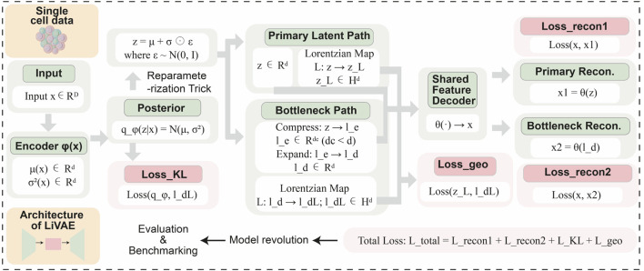 FIGURE 1
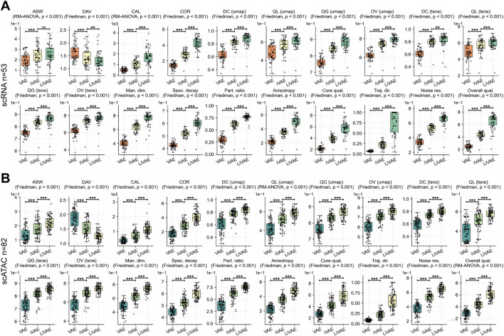 FIGURE 2
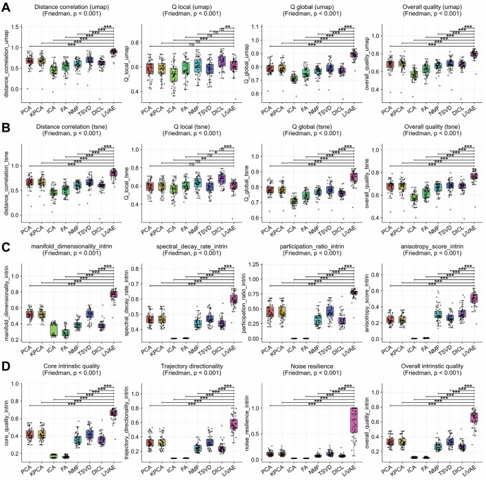 FIGURE 3
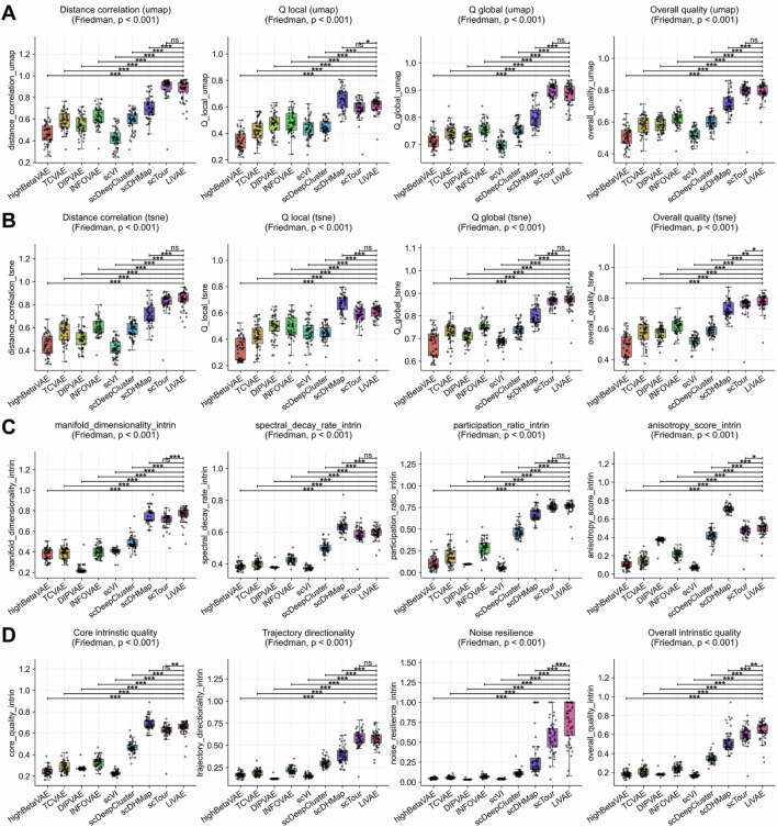 FIGURE 4
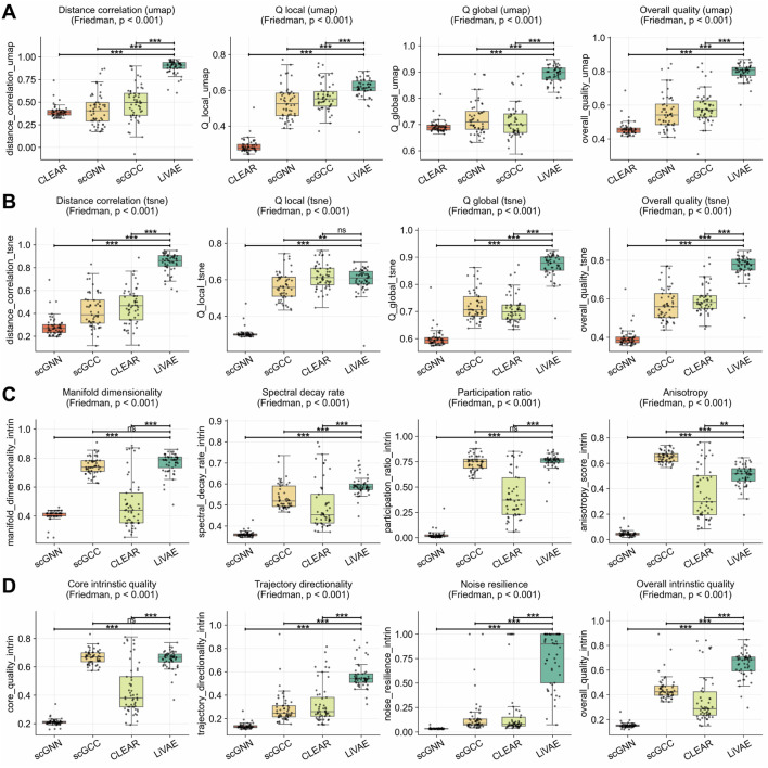 FIGURE 5
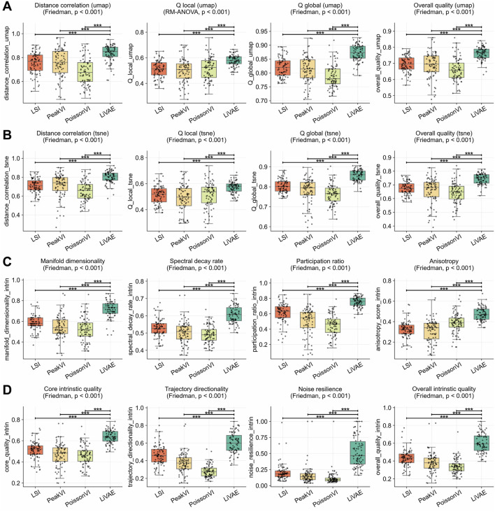 FIGURE 6
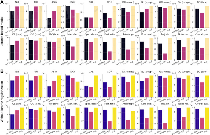 FIGURE 7
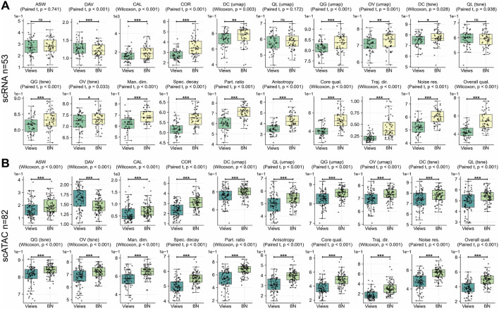 FIGURE 8
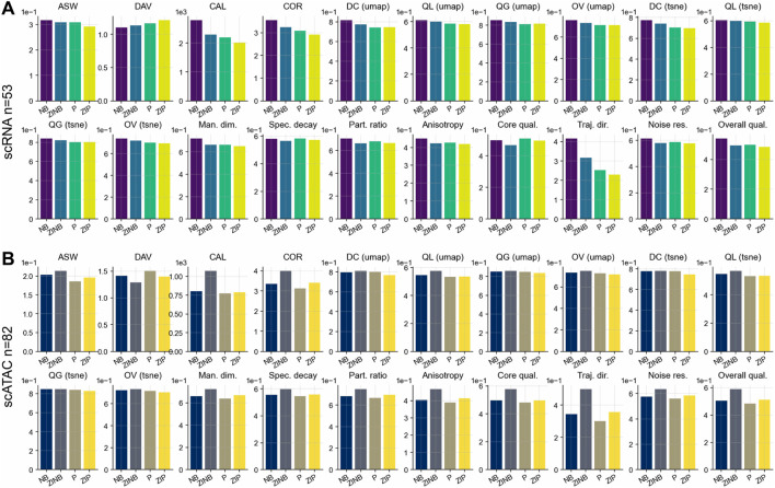 FIGURE 9
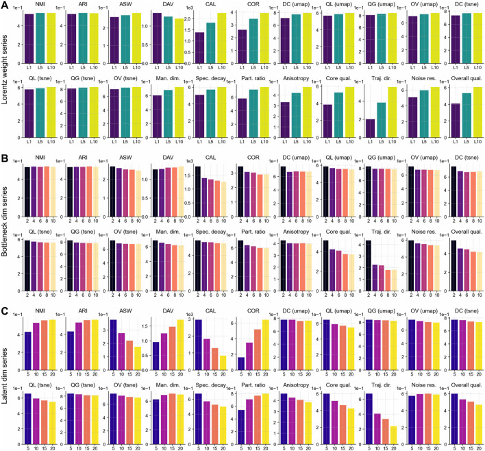 FIGURE 10
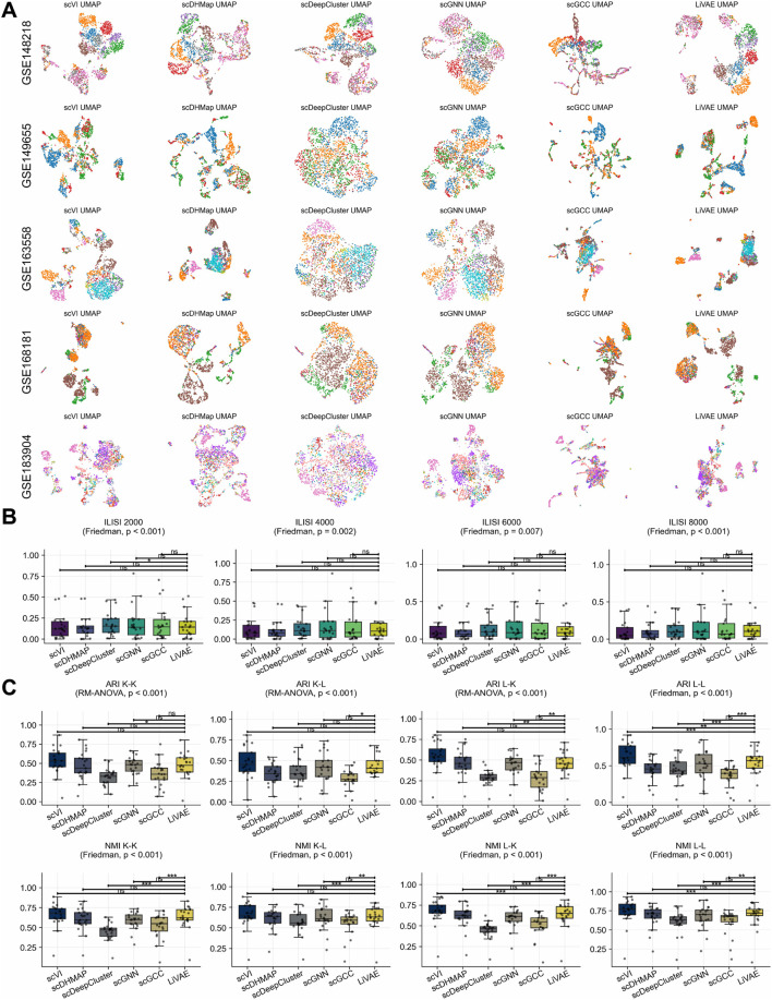 FIGURE 11
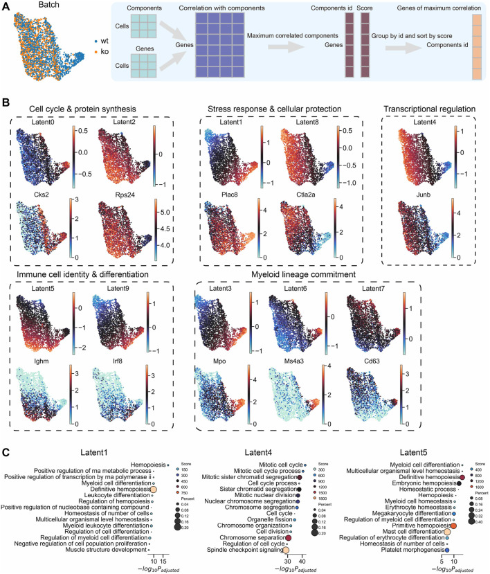 FIGURE 12
| Metric | scRNA-seq | scATAC-seq | ||
|---|---|---|---|---|
| vs. VAE | vs. iVAE | vs. VAE | vs. iVAE | |
|
| ||||
|
|
| 0.009 |
|
|
|
|
|
|
|
|
|
|
|
|
|
|
|
|
|
|
|
|
|
| ||||
|
|
|
|
|
|
|
|
|
|
|
|
|
|
|
|
|
|
|
|
|
|
|
|
|
| ||||
|
|
|
|
|
|
|
|
|
|
|
|
|
|
|
|
|
|
|
|
|
|
|
|
|
| ||||
|
|
|
|
|
|
|
|
|
|
|
|
|
|
|
|
|
|
|
|
|
|
|
|
|
| ||||
|
|
|
|
|
|
|
|
|
|
|
|
|
|
|
|
|
|
|
|
|
|
|
|
| Metric | PCA | KPCA | ICA | FA | NMF | TSVD | DICL |
|---|---|---|---|---|---|---|---|
|
| |||||||
|
|
|
|
|
|
|
|
|
|
| 0.025 | 0.025 |
| 0.029 | 0.002 | 0.027 |
|
|
|
|
|
|
|
|
|
|
|
|
|
|
|
|
|
|
|
|
| |||||||
|
|
|
|
|
|
|
|
|
|
|
| 0.000 |
|
|
| 0.001 |
|
|
|
|
|
|
|
|
|
|
|
|
|
|
|
|
|
|
|
|
| |||||||
|
|
|
|
|
|
|
|
|
|
|
|
|
|
|
|
|
|
|
|
|
|
|
|
|
|
|
|
|
|
|
|
|
|
|
|
|
| |||||||
|
|
|
|
|
|
|
|
|
|
|
|
|
|
|
|
|
|
|
|
|
|
|
|
|
|
|
|
|
|
|
|
|
|
|
|
| Metric |
|
| DIPVAE | InfoVAE | scVI | scDeepCluster | scDHMap | scTour |
|---|---|---|---|---|---|---|---|---|
|
| ||||||||
|
|
|
|
|
|
|
|
|
|
|
|
|
|
|
|
|
|
|
|
|
|
|
|
|
|
|
|
|
|
|
|
|
|
|
|
|
|
|
|
|
| ||||||||
|
|
|
|
|
|
|
|
| 0.024 |
|
|
|
|
|
|
|
|
| 0.022 |
|
|
|
|
|
|
|
|
| 0.008 |
|
|
|
|
|
|
|
|
|
|
|
| ||||||||
|
|
|
|
|
|
|
| 0.016 |
|
|
|
|
|
|
|
|
|
| 0.009 |
|
|
|
|
|
|
|
|
| 0.013 |
|
|
|
|
|
|
|
|
|
|
|
| ||||||||
|
|
|
|
|
|
|
|
|
|
|
|
|
|
|
|
|
|
|
|
|
|
|
|
|
|
|
|
|
|
|
|
|
|
|
|
|
|
|
|
| Metric | vs. CLEAR | vs. scGNN | vs. scGCC |
|---|---|---|---|
|
| |||
|
|
|
|
|
|
|
|
|
|
|
|
|
|
|
|
|
|
|
|
|
| |||
|
|
|
|
|
|
| 0.296 |
|
|
|
|
|
|
|
|
|
|
|
|
|
| |||
|
|
|
| 0.281 |
|
|
|
|
|
|
|
|
| 0.348 |
|
|
|
|
|
|
| |||
|
|
|
| 0.215 |
|
|
|
|
|
|
|
|
|
|
|
|
|
|
|
| Metric | vs. LSI | vs. PeakVI | vs. PoissonVI |
|---|---|---|---|
|
| |||
|
|
|
|
|
|
|
|
|
|
|
|
|
|
|
|
|
|
|
|
|
| |||
|
|
|
|
|
|
|
|
|
|
|
|
|
|
|
|
|
|
|
|
|
| |||
|
|
|
|
|
|
|
|
|
|
|
|
|
|
|
|
|
|
|
|
|
| |||
|
|
|
|
|
|
|
|
|
|
|
|
|
|
|
|
|
|
|
|
| Metric | BN architecture | Lorentz architecture | ||
|---|---|---|---|---|
| vs. w/o main | vs. w/o BN | vs. w/o main | vs. w/o BN | |
|
| ||||
|
| 0.122 | 0.009 | 0.121 | 0.015 |
|
| 0.123 | 0.009 | 0.121 | 0.015 |
|
| 0.142 | 0.062 | 0.129 | 0.062 |
|
|
|
|
|
|
|
| 724.352 | 729.417 | 635.618 | 712.973 |
|
| 0.873 | 1.434 | 0.786 | 1.339 |
|
| ||||
|
| 0.060 | 0.198 | 0.037 | 0.208 |
|
| 0.158 | 0.070 | 0.146 | 0.071 |
|
| 0.031 | 0.077 | 0.025 | 0.079 |
|
| 0.083 | 0.115 | 0.069 | 0.119 |
|
| ||||
|
| 0.088 | 0.223 | 0.052 | 0.227 |
|
| 0.189 | 0.068 | 0.181 | 0.070 |
|
| 0.069 | 0.088 | 0.053 | 0.089 |
|
| 0.115 | 0.126 | 0.095 | 0.129 |
|
| ||||
|
| 0.069 | 0.234 | 0.047 | 0.235 |
|
| 0.017 | 0.095 |
| 0.095 |
|
| 0.106 | 0.355 | 0.057 | 0.356 |
|
|
| 0.151 |
| 0.156 |
|
| ||||
|
| 0.037 | 0.209 | 0.010 | 0.210 |
|
| 0.063 | 0.178 | 0.032 | 0.177 |
|
| 0.050 | 0.141 | 0.020 | 0.132 |
|
| 0.047 | 0.186 | 0.018 | 0.185 |
| Metric | scRNA-seq | scATAC-seq |
|---|---|---|
|
| ||
|
| 0.002 |
|
|
|
|
|
|
|
|
|
|
|
|
|
|
| ||
|
|
|
|
|
| 0.007 |
|
|
|
|
|
|
|
|
|
|
| ||
|
|
|
|
|
|
|
|
|
|
|
|
|
|
|
|
|
| ||
|
|
|
|
|
|
|
|
|
|
|
|
|
|
|
|
|
| ||
|
|
|
|
|
|
|
|
|
|
|
|
|
|
|
|
| Metric | scRNA-seq (NB-based) | scATAC-seq (ZINB-based) | ||||
|---|---|---|---|---|---|---|
| vs. ZINB | vs. Poisson | vs. ZI-Poisson | vs. NB | vs. Poisson | vs. ZI-Poisson | |
|
| ||||||
|
| 0.007 | 0.008 | 0.024 | 0.010 | 0.028 | 0.017 |
|
|
|
|
|
|
|
|
|
| 488.822 | 597.291 | 768.543 | 268.195 | 300.059 | 285.634 |
|
| 0.305 | 0.454 | 0.624 | 0.632 | 0.861 | 0.588 |
|
| ||||||
|
| 0.043 | 0.074 | 0.071 | 0.012 | 0.011 | 0.040 |
|
| 0.011 | 0.025 | 0.029 | 0.029 | 0.042 | 0.040 |
|
| 0.019 | 0.038 | 0.037 | 0.005 | 0.008 | 0.020 |
|
| 0.024 | 0.046 | 0.046 | 0.015 | 0.020 | 0.033 |
|
| ||||||
|
| 0.034 | 0.071 | 0.076 | 0.003 | 0.003 | 0.034 |
|
| 0.004 | 0.011 | 0.018 | 0.021 | 0.037 | 0.035 |
|
| 0.017 | 0.035 | 0.036 | 0.001 | 0.008 | 0.018 |
|
| 0.018 | 0.039 | 0.044 | 0.008 | 0.016 | 0.029 |
|
| ||||||
|
| 0.055 | 0.057 | 0.068 | 0.064 | 0.084 | 0.053 |
|
| 0.014 |
| 0.006 | 0.042 | 0.051 | 0.038 |
|
| 0.043 | 0.023 | 0.039 | 0.063 | 0.082 | 0.052 |
|
| 0.027 | 0.024 | 0.030 | 0.063 | 0.076 | 0.052 |
|
| ||||||
|
| 0.035 | 0.025 | 0.036 | 0.058 | 0.073 | 0.049 |
|
| 0.032 |
| 0.004 | 0.079 | 0.096 | 0.080 |
|
| 0.100 | 0.162 | 0.186 | 0.154 | 0.196 | 0.140 |
|
| 0.047 | 0.042 | 0.056 | 0.084 | 0.105 | 0.076 |
| Metric | Lorentz weight | Bottleneck dim | Latent dim | ||||||
|---|---|---|---|---|---|---|---|---|---|
| vs. L1 | vs. L5 | vs. 4 | vs. 6 | vs. 8 | vs. 10 | vs. 5 | vs. 15 | vs. 20 | |
|
| |||||||||
|
| 0.007 |
|
|
|
|
| 0.101 |
|
|
|
| 0.007 |
|
|
|
|
| 0.100 |
|
|
|
| 0.023 | 0.013 | 0.009 | 0.018 | 0.018 | 0.023 |
| 0.056 | 0.101 |
|
|
|
|
|
|
|
| 0.299 |
|
|
|
| 871.749 | 436.057 | 423.691 | 472.544 | 524.646 | 559.683 |
| 533.832 | 969.863 |
|
| 1.311 | 0.459 | 0.383 | 0.428 | 0.570 | 0.555 | 1.863 |
|
|
|
| |||||||||
|
| 0.080 | 0.024 | 0.085 | 0.077 | 0.081 | 0.079 | 0.003 | 0.021 | 0.016 |
|
| 0.032 | 0.014 | 0.022 | 0.031 | 0.032 | 0.036 |
| 0.019 | 0.043 |
|
| 0.034 | 0.011 | 0.041 | 0.041 | 0.044 | 0.047 |
| 0.005 | 0.011 |
|
| 0.049 | 0.016 | 0.049 | 0.049 | 0.052 | 0.054 |
| 0.015 | 0.023 |
|
| |||||||||
|
| 0.039 | 0.006 | 0.076 | 0.087 | 0.084 | 0.078 |
| 0.021 | 0.030 |
|
| 0.027 | 0.014 | 0.014 | 0.021 | 0.025 | 0.025 |
| 0.025 | 0.042 |
|
| 0.025 | 0.008 | 0.035 | 0.043 | 0.044 | 0.044 |
| 0.013 | 0.016 |
|
| 0.030 | 0.009 | 0.042 | 0.050 | 0.051 | 0.049 |
| 0.020 | 0.029 |
|
| |||||||||
|
| 0.118 | 0.043 | 0.033 | 0.048 | 0.066 | 0.067 | 0.059 |
|
|
|
| 0.093 | 0.030 | 0.020 | 0.021 | 0.032 | 0.034 |
| 0.042 | 0.069 |
|
| 0.168 | 0.039 | 0.065 | 0.082 | 0.107 | 0.110 | 0.166 |
|
|
|
| 0.143 | 0.054 | 0.024 | 0.025 | 0.024 | 0.029 |
| 0.019 | 0.042 |
|
| |||||||||
|
| 0.131 | 0.042 | 0.035 | 0.044 | 0.057 | 0.060 | 0.022 |
| 0.004 |
|
| 0.205 | 0.063 | 0.090 | 0.104 | 0.139 | 0.143 |
| 0.050 | 0.089 |
|
| 0.353 | 0.171 | 0.211 | 0.216 | 0.256 | 0.255 |
| 0.070 | 0.167 |
|
| 0.197 | 0.074 | 0.087 | 0.096 | 0.122 | 0.124 |
| 0.027 | 0.062 |
| Metric | vs. scVI | vs. scDHMap | vs. scDeepCluster | vs. scGNN | vs. scGCC |
|---|---|---|---|---|---|
|
| |||||
|
|
| 0.009 |
| 0.011 | 0.117 |
|
|
| 0.090 | 0.054 | 0.011 |
|
|
|
|
|
| 0.016 |
|
|
|
|
|
| 0.026 |
|
|
| |||||
|
|
| 0.026 |
| 0.041 |
|
|
|
| 0.020 |
| 0.016 |
|
|
|
| 0.017 |
| 0.042 |
|
|
|
| 0.020 |
| 0.024 |
|
Peer Reviews
No public reviews on file for this paper yet. If you reviewed it on a platform where reviews are public (OpenReview, ICLR, NeurIPS, ICML), you can paste yours below so the community can read it here.
Videos
No videos yet. Explain this paper in a talk, walkthrough, or lecture? Add one.
Taxonomy
TopicsSingle-cell and spatial transcriptomics · Pluripotent Stem Cells Research · Genomics and Chromatin Dynamics
Introduction
1
Cellular development unfolds through hierarchical differentiation programs where stem cells progressively commit to specialized fates (Trapnell et al., 2014). Single-cell multi-omics technologies now capture these hierarchies at an unprecedented resolution (Stuart et al., 2019); however, representing tree-like developmental structures computationally remains an open challenge (Luecken et al., 2022). Datasets routinely contain – cells spanning dozens of cell types across tissues (Hao et al., 2021), demanding representations that preserve both fine-grained cell states and global developmental trajectories.
This challenge manifests as a fundamental local–global trade-off: representations must capture fine-grained local neighborhoods for rare cell-type detection (Heiser and Lau, 2020; Kiselev et al., 2019) while maintaining global topology for developmental trajectory inference (Cao et al., 2019; Saelens et al., 2019). Despite advances in deep learning (Hu et al., 2021; Yuan and Kelley, 2022) and foundation models (Cui et al., 2024), most methods excel at one scale at the expense of the other. The tension reflects a geometric limitation of Euclidean spaces: methods optimized for local structure, such as t-distributed stochastic neighbor embedding (t-SNE) (Kobak and Berens, 2019) and uniform manifold approximation and projection (UMAP) (McInnes et al., 2018), distort global topology, while those prioritizing global coherence, such as principal component analysis (PCA) and diffusion maps (Moon et al., 2018; Becht et al., 2019), may obscure fine-grained cell states. Graph-based approaches (Hetzel et al., 2021; Nguyen et al., 2022) and gene co-expression modeling (Deng et al., 2025; Li et al., 2025; Song T. et al., 2022) partially address this by explicitly encoding functional relationships, yet systematic benchmarking reveals that most methods still sacrifice one scale for the other (Tian et al., 2019).
These challenges intensify across modalities: single-cell ATAC sequencing (scATAC-seq) exhibits 90%–95% zero rates versus 60%–80% in single-cell RNA sequencing (scRNA-seq) (Chen et al., 2019; Fang et al., 2021), thus requiring flexible architectures that generalize without extensive re-engineering (Song Q. et al., 2022; Zhao et al., 2024). Hyperbolic geometry offers a principled solution as its exponential volume growth naturally accommodates tree-like hierarchies common in developmental biology (Nickel and Kiela, 2017; Chami et al., 2019; Sarkar, 2012; Bronstein et al., 2021). Existing hyperbolic deep learning methods have improved visualization and captured cellular relationships (Tian et al., 2023; Klimovskaia et al., 2020), but they constrain entire latent spaces to hyperbolic manifolds (Mathieu et al., 2019; Nagano et al., 2019), thus sacrificing compatibility with standard neural architectures and downstream analytical tools. This failure stems from representational constraints: embedding nodes in a balanced binary tree requires Euclidean dimensions to avoid distortion, whereas hyperbolic space requires only dimensions.
We introduce the Lorentz-regularized variational autoencoder (LiVAE), which applies hyperbolic geometry as regularization over standard Euclidean latent representations rather than constraining the latent space itself. LiVAE learns a primary embedding optimized for reconstruction, while a bottleneck (BN) pathway compresses to (where ) and reconstructs . A geometric loss enforces that Lorentzian distances—computed after projecting to the hyperboloid model (Ganea et al., 2018; Skopek et al., 2019)—between and remain small, preserving hierarchical structure while maintaining compatibility with downstream tools. This design resolves the local–global tension through complementary objectives: the information bottleneck (Tishby and Zaslavsky, 2015; Strouse and Schwab, 2017) discards technical noise while retaining biological structure, implicitly promoting cross-sample integration (Lopez et al., 2018; Lynch et al., 2023), while the dual reconstruction paths balance local fidelity (primary path from ) with global coherence (bottleneck path via ).
We validate LiVAE on 135 datasets spanning scRNA-seq and scATAC-seq against 21 baseline methods using 12 metrics assessing embedding fidelity, manifold geometry, and robustness. LiVAE consistently achieves superior global topology preservation and noise resilience while remaining competitive on local structure metrics. Component-wise interpretability analysis demonstrates that latent dimensions decompose into biologically meaningful axes corresponding to cell cycle, immune identity, and differentiation programs (Choi et al., 2023; Madrigal et al., 2024).
Our contributions are threefold: (1) architectural innovation: a hybrid design applying hyperbolic regularization to Euclidean representations via information bottlenecks, balancing local fidelity with global coherence; (2) cross-modality generalization: a unified framework handling scRNA-seq and scATAC-seq through modality-appropriate likelihoods without architectural changes; and (3) biological interpretability: latent dimensions aligned with known biological processes that enable mechanistic hypothesis generation beyond black-box embeddings. By resolving the local–global trade-off through geometric regularization, LiVAE provides a flexible foundation for single-cell multi-omics analysis that preserves biological hierarchy without sacrificing compatibility with existing computational workflows.
Materials and methods
2
Notation
2.1
Throughout this section, denotes a batch of cells with features, denotes a single cell, and denotes a scalar value (gene or peak in cell ). Latent representations include (batch) and (single cell). The dimensions are (latent dimension) and (bottleneck dimension, where ). Lorentzian projections are denoted as (hyperboloid manifold).
LiVAE architecture overview
2.2
LiVAE is a variational autoencoder that applies Lorentzian geometric regularization across a dual-pathway latent space architecture (Figure 1). The encoder maps the input to a diagonal Gaussian posterior . A latent vector is sampled via reparameterization and processed through two parallel pathways: (1) the primary path uses directly for reconstruction and geometric comparison; (2) the bottleneck path compresses to (where ) and expands it back to . A shared decoder reconstructs from both the representations, yielding and .
LiVAE architecture. Input x is encoded to latent z , which is processed via two pathways: (1) primary path: direct Lorentzian projection (zH) ; (2) bottleneck path: compression to le (dimension dc≪d ), expansion to ld , and Lorentzian projection to (ldH) . Shared decoder θ reconstructs from both z and ld . The total loss combines two reconstruction terms (Lrecon1,Lrecon2) , KL divergence (LKL) , and geometric loss (Lgeo) enforcing Lorentzian distance preservation.
The model is trained via total loss comprising two reconstruction losses , Kullback–Leibler (KL) divergence , and a geometric loss that enforces Lorentzian distance preservation between and after mapping to the hyperbolic space.
Model architecture
2.3
Encoder network
2.3.1
For each cell in batch , the encoder outputs the mean and log-variance (Equation 1). Latent vectors are sampled as follows:
and . The encoder consists of a single hidden layer with 128 units, ReLU activation, and layer normalization.
Dual latent pathways and decoder
2.3.2
The bottleneck path applies two linear transformations: compression (to dimension ) and expansion (back to dimension ), where and , producing compressed representation and expanded representation .
The decoder mirrors the encoder architecture, outputting distribution parameters via linear layers followed by softmax normalization. It generates two reconstructions:
- Primary reconstruction: .
- Bottleneck reconstruction: .
Loss function
2.4
The total loss function (Equation 2) is a weighted sum of four components:
where and are hyperparameters balancing the regularization terms.
Reconstruction losses
2.4.1
The reconstruction losses (Equation 3) measure how well each pathway captures the input:
The likelihood is modality-specific.
- scRNA-seq: negative binomial (NB) distribution with the mean (decoder output scaled by the cell library size) and gene-specific dispersion parameter to model count overdispersion.
- scATAC-seq: zero-inflated negative binomial (ZINB) with additional zero-inflation probability from a separate decoder head, accounting for excess zeros in chromatin accessibility (90%–95% sparsity vs. 60%–80% in scRNA-seq).
- Alternative: Poisson and zero-inflated Poisson (ZIP) likelihoods are also supported for datasets with minimal overdispersion.
For all likelihoods, the predicted means are obtained as , where the decoder output is normalized by the cell-wise library size.
Kullback–Leibler divergence
2.4.2
The KL divergence is the standard variational autoencoder (VAE) regularizer that encourages the posterior to approximate a unit Gaussian prior (Equation 4):
Geometric loss
2.4.3
The geometric loss enforces that the bottleneck transformation preserves the hyperbolic geometric structure. Euclidean vectors and are mapped to the hyperboloid (the Lorentzian model of hyperbolic space) via the exponential map at origin (Equation 5):
where is a tangent vector with the first coordinate zero.
The geometric loss is the mean squared Lorentzian distance between paired representations (Equation 6):
where and , and the Lorentzian distance is obtained as follows (Equation 7):
with the Lorentzian inner product . For numerical stability, we use when , with clamping .
Evaluation metrics
2.5
We assess LiVAE performance using 12 metrics organized into four categories, evaluating complementary aspects of representation quality.
Clustering quality metrics
2.5.1
We assess the biological population structure using five standard metrics and one novel metric:
Standard metrics: Normalized mutual information (NMI) and adjusted Rand index (ARI) measure agreement between the predicted clusters and ground-truth cell-type labels, with values near 1 indicating strong correspondence. Average silhouette width (ASW) and the Calinski–Harabasz index (CAL) quantify cluster cohesion and separation (higher is better), while the Davies–Bouldin index (DAV) measures the average cluster similarity (lower is better). These metrics are computed using standard implementations in scikit-learn.
Coupling degree (COR) (Equation 8): We introduce this metric to quantify preservation of interdependent biological programs:
where is the Pearson correlation between latent dimensions and and is the latent space dimensionality. Higher COR values indicate stronger coupling, reflecting coordinated gene expression programs that are essential for continuous differentiation trajectories.
Dimensionality reduction embedding quality metrics
2.5.2
We evaluate how effectively latent representations project to interpretable low-dimensional spaces (UMAP and t-SNE) while preserving biological relationships.
Distance correlation (Equation 9) quantifies the preservation of pairwise distance relationships:
where and are pairwise Euclidean distance matrices in latent and embedding spaces, respectively, vectorizes the upper triangle, and is the Spearman rank correlation coefficient. Higher values indicate better preservation of the global structure.
Local quality and global quality (Equation 10) measure preservation at different scales through co-ranking matrix analysis:
where is the normalized co-ranking quality measure at neighborhood size and is the optimal local neighborhood boundary. Higher values indicate better maintenance of local neighborhoods and large-scale topology, respectively.
Overall embedding quality (Equation 11) combines the three components:
Intrinsic manifold quality metrics
2.5.3
We characterize geometric properties of the latent manifold through spectral analysis of the covariance matrix , with eigenvalues .
Manifold dimensionality (Equation 12) measures representation compactness:
where represents the number of principal components explaining 95% variance. Higher values indicate more efficient encoding.
Spectral decay rate (Equation 13) quantifies hierarchical structure clarity:
where is the slope from log-linear regression on eigenvalues. Higher values indicate steeper spectrum decay, reflecting clear hierarchical organization.
Participation ratio (Equation 14) assesses the balance of variance distribution:
Higher values indicate more uniform utilization of latent dimensions, thereby preventing dimension collapse.
Anisotropy score (Equation 15) quantifies directional bias strength:
where . Higher values indicate stronger directional structure along the dominant axes, which is essential for trajectory representation.
Trajectory directionality (Equation 16) measures dominance of the primary variation axis:
Higher values indicate a single dominant trajectory, which is characteristic of linear differentiation processes.
Noise resilience (Equation 17) approximates the signal-to-noise ratio:
Higher values indicate robust separation between signal and noise subspaces.
Composite scores.
We define two summary metrics: core intrinsic quality (Equation 18) integrates the fundamental geometric properties,
while overall intrinsic quality (Equation 19) incorporates task-oriented components with weights :
Batch integration quality
2.5.4
The integration local inverse Simpson index (iLISI) (Equation 20) measures batch mixing quality. For each cell ,
where represents the number of batches and represents the proportion of cell ’s -nearest neighbors from batch , and it is computed using a Gaussian kernel with the bandwidth determined by perplexity. The overall score is . Higher values (approaching ) indicate better batch integration, while values near 1 indicate poor mixing.
Datasets and preprocessing
2.6
Dataset selection
2.6.1
We curated 135 single-cell datasets from public repositories (Gene Expression Omnibus, GEO): 53 scRNA-seq dataset and 82 scATAC-seq dataset samples. Raw single-cell count matrices underwent quality control and normalization prior to model training. Both modalities require raw integer counts as input as the model employs count-based likelihood functions.
scRNA-seq preprocessing
2.6.2
The top 5,000 highly variable genes (HVGs) were selected by modeling the mean–variance relationship in count data. For model input, normalized data were obtained by applying transformation, followed by -score standardization with outlier clipping at standard deviations.
scATAC-seq preprocessing
2.6.3
Term frequency–inverse document frequency (TF-IDF) normalization (Equation 21) was applied:
where the term frequency for cell and peak is , the inverse document frequency is , with being the total number of cells and being the number of cells where peak is accessible, and is a scaling factor. Highly variable peaks (HVPs) were identified using variance-based selection on TF-IDF normalized values, which were restricted to peaks with accessibility between 1% and 95% of cells. The top 10,000 HVPs were selected as input features.
Model hyperparameters
2.7
LiVAE was configured with the following default hyperparameters. The encoder and decoder networks each contained a single hidden layer of dimension 128. The latent space dimension was set to , and the information bottleneck dimension was set to . The loss function weights were the primary reconstruction weight , bottleneck reconstruction weight , KL divergence weight , and geometric loss weight . For reconstruction losses, we employed NB likelihood for scRNA-seq data and ZINB likelihood for scATAC-seq data. Training was performed using the Adam optimizer with a learning rate of and a batch size of 128. Gradient clipping with a threshold of 1.0 was applied. Layer normalization was employed in both the encoder and decoder networks.
Baseline methods
2.8
We compared LiVAE against 21 methods spanning four categories:
- Classical dimensionality reduction (seven methods): PCA, kernel PCA (KPCA), factor analysis (FA), non-negative matrix factorization (NMF), independent component analysis (ICA), truncated SVD (TSVD), and dictionary learning (DICL).
- Deep generative models (eight methods): standard VAE, -variational autoencoder ( -VAE), total correlation -VAE ( -TCVAE), disentangled inferred prior VAE (DIPVAE), information maximizing VAE (InfoVAE), single-cell variational inference (scVI), single-cell deep clustering (scDeepCluster), single-cell deep hyperbolic manifold learning (scDHMap), and single-cell trajectory optimization (scTour).
- Graph and contrastive learning (three methods): contrastive learning for scRNA-seq (CLEAR), single-cell graph neural network (scGNN), and single-cell graph contrastive clustering (scGCC).
- Modality-specific methods (three methods): latent semantic indexing (LSI), peak variational inference (PeakVI), and Poisson variational inference (PoissonVI) for scATAC-seq.
Statistical analysis
2.9
We used paired experimental designs (identical datasets for all methods). For each metric, normality was assessed using the Shapiro–Wilk test . Multi-method comparisons employed repeated measures analysis of variance (ANOVA) (normal data) or Friedman test (non-normal), followed by Tukey honest significant difference (HSD) or Bonferroni-corrected Wilcoxon signed-rank post hoc tests, respectively. The significance levels were * , ** , and *** .
Results
3
Architectural progression from foundational VAEs yields comprehensive performance gains
3.1
We benchmarked LiVAE against its foundational predecessors—standard VAE and information bottleneck VAE (iVAE)—using 135 datasets (53 scRNA-seq and 82 scATAC-seq). LiVAE’s complete architecture established a new performance baseline, delivering statistically significant improvements across nearly all metrics for both scRNA-seq (Figure 2A) and scATAC-seq datasets (Figure 2B; Table 1).
Progressive architectural enhancements yield consistent performance gains. Boxplots display performance differences ( Δ ; LiVAE − baseline) across five evaluation categories. Statistical significance was assessed using Tukey’s HSD post hoc test for ASW and CAL (scRNA-seq), Q local (UMAP), and overall intrinsic quality (scATAC-seq); Bonferroni-corrected Wilcoxon signed-rank tests were applied for all other metrics. Boxes indicate the median and IQR; whiskers extend to 1.5× IQR. Statistical methods are indicated in subplot titles. (A) scRNA-seq datasets (n=53) . (B) scATAC-seq datasets (n=82) .
**TABLE 1: Performance differences between LiVAE and baseline VAE models across scRNA-seq (n=53) and scATAC-seq (n=82) datasets. Values represent absolute differences ( Δ ; LiVAE − baseline). Significance levels: ***
p<0.001 , **
p<0.01 , and *
p<0.05 .**
The most striking advantage was a profound increase in model robustness. For scRNA-seq (Figure 2A), LiVAE boosted noise resilience by (vs. VAE) and (vs. iVAE), translating to superior overall intrinsic quality ( and , respectively; all ). Comparable patterns were obtained for scATAC-seq (Figure 2B), with noise resilience gains of and , and overall intrinsic quality improvements of and .
This enhanced robustness stemmed from LiVAE’s geometrically expressive latent space. For scRNA-seq, the participation ratio increased by (vs. VAE) and (vs. iVAE), while manifold dimensionality, spectral decay, and anisotropy improved by , , and , respectively. Similar gains were obtained for scATAC-seq (Table 1). These structural improvements enabled faithful visualizations, with UMAP distance correlation increasing by (scRNA-seq) and (scATAC-seq). Clustering performance improved dramatically; for scRNA-seq, cluster alignment (CAL) increased by (vs. VAE) and (vs. iVAE), while latent dimension coupling (COR) increased by and (all ), indicating stronger preservation of coordinated biological programs. Collectively, these results demonstrate that LiVAE’s components—bottleneck, dual-pathway loss, and Lorentz regularization—synergistically create a more stable, powerful, and biologically informative model.
Balanced profile of local fidelity and global structure against classical methods
3.2
We benchmarked LiVAE against seven classical algorithms on scRNA-seq datasets. While some classical methods showed competitive local neighborhood preservation, LiVAE provided superior global coherence, manifold complexity, and robustness (Table 2).
**TABLE 2: Performance differences between LiVAE and classical dimensionality reduction methods across n=53 scRNA-seq datasets. Values represent absolute differences ( Δ ; LiVAE − baseline). Significance levels: ***
p<0.001 , **
p<0.01 , and *
p<0.05 .**
LiVAE’s UMAP local quality (Figure 3A) was statistically equivalent to those of PCA, KPCA, FA, NMF, and TSVD but slightly lower than that of dictionary learning (DICL; , ) and ICA . However, LiVAE demonstrated massive advantages in global structure, with UMAP distance correlation surpassing all methods by (vs. TSVD) to (vs. ICA), yielding overall UMAP quality gains of to (all ). Parallel trends emerged for t-SNE (Figure 3B), with distance correlation improvements of to and overall quality gains of to .
Balanced local–global performance relative to classical dimensionality reduction. Boxplots summarize metric distributions for LiVAE and seven classical baselines across n=53 scRNA-seq datasets. Boxes indicate the median and IQR; whiskers extend to 1.5× IQR. Statistical significance was assessed using Bonferroni-corrected Wilcoxon tests (α=0.0018) . (A) UMAP embedding fidelity. (B) t-SNE embedding fidelity. (C) Latent manifold structure. (D) Intrinsic quality and robustness.
This superior organization reflected a sophisticated latent space (Figure 3C). All four manifold metrics improved substantially: dimensionality ( to ), spectral decay ( to ), participation ratio ( to ), and anisotropy ( to ). Critically, noise resilience exceeded that of all classical methods ( to ; Figure 3D), culminating in overall intrinsic quality gains of to (all ). Thus, LiVAE delivers a balanced, robust solution for single-cell exploratory analysis.
Competitive edge in stability and manifold quality against state-of-the-art generative models
3.3
We assessed LiVAE against eight state-of-the-art deep generative models on scRNA-seq datasets, confirming it as a top-tier general-purpose embedding method distinguished by exceptional stability and global latent-space integrity (Table 3).
**TABLE 3: Performance differences between LiVAE and advanced generative and scRNA-seq-specialized methods across n=53 scRNA-seq datasets. Values represent absolute differences ( Δ ; LiVAE − baseline). Significance levels: ***
p<0.001 , **
p<0.01 , and *
p<0.05 .**
While trajectory-focused models such as scTour achieved UMAP distance correlation (Figure 4A) statistically equivalent to LiVAE’s ( , n.s.), LiVAE consistently outperformed the majority across nearly all metrics. Its paramount advantage was robustness: noise resilience exceeded all eight competitors by (vs. scTour) to (vs. DIPVAE; Figure 4D), fostering overall intrinsic quality gains of to (all ).
Enhanced global fidelity and stability versus advanced deep generative models. Boxplots compare LiVAE with eight state-of-the-art baselines across n=53 scRNA-seq datasets. Boxes indicate the median and IQR; whiskers extend to 1.5× IQR. Statistical significance was assessed using Bonferroni-corrected Wilcoxon tests (α=0.0014) . (A) UMAP embedding fidelity. (B) t-SNE embedding fidelity. (C) Latent manifold structure. (D) Intrinsic quality and robustness.
These strengths translated into superior geometric organization. LiVAE delivered UMAP overall quality improvements of to (Figure 4A), with distance correlation gains of to (except scTour). The participation ratio consistently exceeded that of all methods ( to ; Figure 4C), indicating richer manifold complexity. While specialized models such as scDHMap yielded higher anisotropy , reflecting trajectory optimization, LiVAE provided a state-of-the-art balance of local fidelity (Figures 4A,B), global structure, and best-in-class robustness, making it ideal for broad single-cell data exploration.
Implicit geometric regularization is comparable to explicit graph-based architectures
3.4
We benchmarked LiVAE against three prominent graph-aware models (CLEAR, scGNN, and scGCC) on scRNA-seq datasets. LiVAE’s implicit geometric regularization matched or exceeded explicit graph-based methods, particularly in global fidelity and robustness (Table 4).
**TABLE 4: Performance differences between LiVAE and graph-based deep learning methods across n=53 scRNA-seq datasets. Values represent absolute differences ( Δ ; LiVAE − baseline). Significance levels: ***
p<0.001 , **
p<0.01 , and *
p<0.05 .**
Despite the graph-based models’ design for local structure, LiVAE proved highly competitive, significantly outperforming CLEAR , scGNN , and scGCC in UMAP local quality (all ; Figure 5A). LiVAE established commanding leads in global embedding fidelity, with UMAP distance correlation improvements of to , yielding overall UMAP quality gains of to . The t-SNE results (Figure 5B) paralleled these findings ( to for overall quality).
Strong embedding quality and robustness without explicit graph regularization. Boxplots compare LiVAE with three graph-based baselines across n=53 scRNA-seq datasets. Boxes indicate the median and IQR; whiskers extend to 1.5× IQR. Statistical significance was assessed using Bonferroni-corrected Wilcoxon tests (α=0.0083) . (A) UMAP embedding fidelity. (B) t-SNE embedding fidelity. (C) Latent manifold structure. (D) Intrinsic quality and robustness.
Model stability was exceptional, with noise resilience substantially higher than that of all comparators ( to , all ; Figure 5D). Manifold complexity (Figure 5C) surpassed CLEAR across all metrics; comparisons with scGCC for dimensionality and the participation ratio showed numerical advantages not reaching statistical significance. While scGNN produced higher anisotropy , LiVAE produced superior overall intrinsic quality ( to ; Figure 5D), demonstrating that Lorentz-regularized information bottlenecks provide a powerful alternative to graph-based regularization.
Versatile and robust performance on chromatin accessibility data
3.5
We evaluated LiVAE on scATAC-seq data against three specialized methods (LSI, PeakVI, and PoissonVI) across datasets, demonstrating its cross-modality versatility and unique strengths in capturing the global structure and trajectory information (Table 5).
**TABLE 5: Performance differences between LiVAE and scATAC-seq-specialized methods across n=82 scATAC-seq datasets. Values represent absolute differences ( Δ ; LiVAE − baseline). Significance levels: ***
p<0.001 , **
p<0.01 , and *
p<0.05 .**
Against LSI and PeakVI, LiVAE was unequivocally superior across all categories. Overall intrinsic quality (Figure 6D) improved by and , driven by noise resilience gains of and , confirming robustness to sparse chromatin data. Manifold structure (Figure 6C) exceeded both methods across all four metrics: dimensionality , spectral decay , participation ratio , and anisotropy ( , all ).
Comparison with scATAC-seq-specialized methods. Boxplots compare LiVAE with LSI, PeakVI, and PoissonVI across n=82 scATAC-seq datasets. Boxes indicate the median and IQR; whiskers extend to 1.5× IQR. Statistical significance was assessed using Bonferroni-corrected Wilcoxon tests (α=0.0083) . (A) UMAP embedding fidelity. (B) t-SNE embedding fidelity. (C) Latent manifold structure. (D) Intrinsic quality and robustness.
The comparison against PoissonVI revealed LiVAE’s complementary strengths. LiVAE achieved higher core intrinsic quality and dramatically superior trajectory directionality ( ; Figure 6D), suggesting better capture of continuous biological processes. Its geometric regularization provided superior global structure (UMAP distance correlation ; Figure 6A) and overall intrinsic quality , alongside exceptional noise resilience ( , all ). These results confirm LiVAE as a powerful tool for scATAC-seq analysis, offering compelling advantages for studies prioritizing global landscape understanding and developmental trajectory inference.
Dual loss pathways provide complementary representational benefits
3.6
We performed ablation studies on scRNA-seq datasets, systematically removing either the main reconstruction or the bottleneck pathway under both BN and Lorentz-regularized configurations. The two pathways perform highly specialized, non-redundant functions, with the full model decisively outperforming any simplified variant (Table 6).
TABLE 6: Performance differences for dual-pathway ablations under bottleneck-only (BN) and Lorentz-regularized (Lorentz) configurations across n=53 scRNA-seq datasets. Values represent absolute differences ( Δ ; full model − ablation). All differences are derived from paired comparisons; formal significance testing was not applied.
Removing the bottleneck pathway (“w/o BN”) caused catastrophic collapse in geometric integrity. Overall intrinsic quality increased by (BN; Figure 7A) and (Lorentz; Figure 7B), while the participation ratio decreased by . UMAP distance correlation declined by , with overall quality decreasing by . Remarkably, supervised clustering (NMI/ARI) declined minimally , demonstrating the bottleneck’s primary role in establishing geometric robustness rather than defining discrete clusters.
Ablation analysis of dual loss pathways. (A) Bottleneck-only configuration (BN): full model vs. w/o main and w/o BN, n=53 scRNA-seq datasets. (B) Lorentz-regularized configuration (Lorentz): full model vs. w/o main and w/o BN, n=53 scRNA-seq datasets.
Conversely, removing the main pathway (“w/o main”) produced an inverted deficiency profile. Supervised clustering accuracy collapsed (NMI/ARI ; CAL –724), while intrinsic quality and manifold structure worsened less severely. This indicates that the main pathway refines latent space for categorical label separation, operating upon the bottleneck’s stable geometric foundation. These complementary roles prove that both pathways are indispensable for state-of-the-art performance.
A deterministic anchor point fortifies geometric regularization
3.7
To establish the most effective method for applying Lorentz-distance regularization, we contrasted two strategies: anchoring the calculation to the deterministic information BN versus using two independently sampled posterior views (Views). Evaluation on scRNA-seq and scATAC-seq datasets revealed that the bottleneck-anchored strategy was superior across all metric categories (Figures 8A,B; Table 7).
Comparison of Lorentz-regularization strategies. (A) scRNA-seq (n=53) : bottleneck-anchored (BN) vs. two-view sampled (Views). (B) scATAC-seq (n=82) : BN vs. Views.
**TABLE 7: Performance differences between bottleneck-anchored (BN) and two-view sampled (Views) Lorentz regularization across scRNA-seq (n=53) and scATAC-seq (n=82) datasets. Values represent absolute differences ( Δ ; BN − Views). Significance levels: ***
p<0.001 , **
p<0.01 , and *
p<0.05 .**
The BN approach’s most profound impact was on model robustness and manifold quality. Noise resilience increased dramatically ( for scRNA-seq; for scATAC-seq), driving overall intrinsic quality gains of and , respectively. This stability was mirrored in latent geometry: participation ratio improved by and , respectively; manifold dimensionality improved by for both modalities; and trajectory directionality improved by and , respectively. These structural gains translated to better embedding fidelity (UMAP overall quality: and ; t-SNE: and ), improved cluster compactness (CAL: and ), and enhanced latent dimension coupling (COR: and ), indicating stronger preservation of coordinated biological programs. The average silhouette width showed minimal change for scRNA-seq but notable improvement for scATAC-seq .
These results indicate that anchoring Lorentz regularization to a fixed, deterministic reference point mitigates training instability inherent in stochastic sampling. The bottleneck provides a consistent geometric scaffold, enabling more coherent latent organization across all analysis modalities.
Optimizing data fidelity through modality-aware reconstruction
3.8
Selecting an appropriate reconstruction loss is crucial for modeling distinct single-cell assay properties. We benchmarked four likelihoods—NB, ZINB, Poisson, and ZI-Poisson—on scRNA-seq and scATAC-seq datasets (Figures 9A,B; Table 8).
Evaluation of reconstruction likelihood functions. (A) scRNA-seq (n=53) : LiVAE with NB, ZINB, Poisson, and ZI-Poisson. (B) scATAC-seq (n=82) : LiVAE with NB, ZINB, Poisson, and ZI-Poisson.
TABLE 8: Performance differences for reconstruction likelihood functions across scRNA-seq (n=53) and scATAC-seq (n=82) datasets. Values represent absolute differences ( Δ ; optimal loss − alternative). For scRNA-seq: NB vs. others; for scATAC-seq: ZINB vs. others. All differences are derived from paired comparisons; formal significance testing was not applied.
For scRNA-seq, NB provided the most robust performance (Figure 9A). Its primary advantage was enhanced noise resilience ( to vs. alternatives) and overall intrinsic quality ( to ), translating to superior cluster compactness (CAL: up to 768.543) and stronger latent dimension coupling (COR: up to 0.624), reflecting better preservation of interdependent biological programs. Embedding fidelity showed consistent but modest improvements (UMAP overall quality: to ). While Poisson achieved marginal advantages in trajectory directionality and spectral decay , NB’s robustness benefits outweighed these task-specific trade-offs. The NB distribution effectively models the overdispersion characteristic of gene expression without requiring explicit zero-inflation handling.
For scATAC-seq, ZINB was superior (Figure 9B), driven by better noise resilience ( up to 0.196) and manifold structure (participation ratio: vs. NB). ZINB achieved stronger latent dimension coupling (COR: vs. NB), indicating better preservation of coordinated regulatory programs and higher overall intrinsic quality ( vs. NB, vs. Poisson). This advantage reflects ZINB’s ability to explicitly model both overdispersion and the extreme zero-inflation inherent in sparse chromatin accessibility data, making it essential for accurate scATAC-seq representation.
Robustness and hyperparameter stability
3.9
We evaluated LiVAE’s sensitivity to key hyperparameters on scRNA-seq datasets: Lorentz-regularization weight , bottleneck dimensionality , and latent dimensionality , which are visualized in Figures 10A–C and quantified in Table 9.
Hyperparameter sensitivity analysis. (A) Lorentz-regularization weight (λ∈{1,5,10}) on n=53 scRNA-seq datasets. (B) Information bottleneck dimensionality (dBN∈{2,4,6,8,10}) on n=53 scRNA-seq datasets. (C) Latent dimensionality (dlatent∈{5,10,15,20}) on n=53 scRNA-seq datasets.
TABLE 9: Performance differences for hyperparameter ablations across n=53 scRNA-seq datasets. Values represent absolute differences ( Δ ; optimal setting − alternative). Lorentz weight: λ=10 vs. others; bottleneck dim.: dBN=2 vs. others; latent dim.: dlatent=10 vs. others. All differences are derived from paired comparisons; formal significance testing was not applied.
Increasing from 1 to 10 consistently improved performance (Figure 10A), particularly overall intrinsic quality , driven by gains in noise resilience , trajectory directionality , and the participation ratio . Clustering compactness (CAL: ) and embedding fidelity (UMAP overall quality: ) also improved. Moving from to showed diminishing but positive returns across most metrics, suggesting that stronger regularization is generally beneficial.
The bottleneck dimensionality analysis revealed that achieved optimal performance in unsupervised metrics (Figure 10B). Compared to , it improved clustering compactness (CAL: ), embedding quality (UMAP: ; t-SNE: ), and manifold structure (participation ratio: ), with minimal impact on supervised clustering (NMI: ). This tight bottleneck effectively isolates core biological signals while filtering technical noise.
Latent dimensionality presented a clear trade-off (Figure 10C). The setting balanced supervised clustering accuracy (NMI: vs. ; vs. ) with unsupervised compactness. Lower dimensions underfit the complex structure, while higher dimensions reduced cluster compactness (CAL: worse than ) and weakened latent dimension coupling (COR: ), suggesting diminished preservation of coordinated biological programs.
These findings support the default settings of , , and for typical analyses, with adjustable based on the dataset complexity.
Emergent batch correction and robust clustering performance
3.10
LiVAE’s information bottleneck and geometric regularization promote globally coherent embeddings that can disentangle biological signals from batch effects without explicit batch-correction terms. We benchmarked multi-batch scRNA-seq integration against scVI, scDHMap, scDeepCluster, scGNN, and scGCC on 21 multi-batch datasets.
UMAP visualizations of five representative datasets show well-mixed embeddings preserving biological structure (Figure 11A). Quantitative iLISI evaluation across the full set of 21 datasets with 2,000–8,000 cell subsamplings revealed that LiVAE achieves batch mixing comparable to that with specialized methods (Figure 11B).
Batch integration and supervised clustering across multi-batch scRNA-seq datasets. (A) Representative UMAP embeddings from LiVAE and five comparison methods across five multi-batch datasets, colored by batch. (B) iLISI evaluation across downsampled cell counts (2,000–8,000); LiVAE achieves comparable batch mixing to specialized methods across n=21 datasets. (C) Supervised clustering accuracy (ARI and NMI) using four combinations of pre- and post-clustering algorithms: K-means/K-means (K–K), K-means/Leiden (K–L), Leiden/K-means (L–K), and Leiden/Leiden (L–L).
Supervised clustering evaluation using four pipelines—combining K-means or Leiden for pre- and post-integration clustering (denoted as K–K, K–L, L–K, and L–L)—showed mixed results (Figure 11C; Table 10). LiVAE substantially outperformed scDeepCluster (ARI: to ) and scGCC ( to ) across most pipelines. However, scVI achieved superior accuracy in Leiden-based strategies (ARI: to ; NMI: to ).
**TABLE 10: Paired differences in supervised clustering across four clustering strategies evaluated on multi-batch single-cell datasets ( n=21 experimental conditions from five datasets). Values represent absolute differences ( Δ ; LiVAE − comparator). Significance levels: *
p<0.05 , **
p<0.01 , and ***
p<0.001 . Negative values with markers indicate significant superiority of the comparator; positive values with markers indicate significant superiority of LiVAE. Absence of markers indicates non-significant differences.**
These findings demonstrate that LiVAE provides competitive batch integration and stable clustering without specialized batch parameters. Although dedicated batch-correction methods may be preferred for datasets with extreme confounding, LiVAE offers a versatile, general-purpose solution for integrated single-cell analysis.
Biological interpretability of latent components on a Dapp1 perturbation dataset
3.11
To assess LiVAE’s biological interpretability, we analyzed hematopoietic stem and progenitor cell scRNA-seq with Dapp1 knockout perturbation (GSE277292). UMAP embedding showed consistent cellular structure with minimal batch effects between wild-type and knockout conditions (Figure 12A). We annotated components by identifying genes with the highest per-cell expression–activation correlation.
Interpretability of LiVAE latent components in a Dapp1 perturbation scRNA-seq dataset. (A) UMAP of cells from GSE277292, colored by condition (wt: wild-type; ko: knockout), and schematic of the gene-component association workflow based on the maximum expression correlation. (B) UMAPs of selected component activation scores (top of each pair) alongside expression of the most correlated marker genes (bottom). Functional groupings include cell cycle and protein synthesis (Latent0/Cks2 and Latent2/Rps24); stress response and cellular protection (Latent1/Plac8 and Latent8/Ctla2a); transcriptional regulation (Latent4/Junb); immune identity and differentiation (Latent5/Ighm and Latent9/Irf8); and myeloid lineage commitment (Latent3/Mpo, Latent6/Ms4a3, and Latent7/Cd63). (C) Gene Ontology biological process (GOBP) enrichment for the top correlated genes with Latent1, Latent4, and Latent5. Dot size indicates the gene count; color encodes adjusted p -value. Results support roles in hemopoiesis, mitotic cell-cycle processes, and myeloid differentiation.
Individual components captured distinct biological programs (Figure 12B). Cell-cycle and protein synthesis were tracked by Latent0 (Cks2) and Latent2 (Rps24). Stress-response programs aligned with Latent1 [Plac8 (Rogulski et al., 2005)] and Latent8 (Ctla2a). Transcriptional regulation was reflected in Latent4 [Junb (Santilli et al., 2021)]. Immune identity was found through Latent5 [Ighm (Dobre et al., 2021)] and Latent9 [Irf8 (Kurotaki and Tamura, 2019)], while myeloid commitment was found through Latent3 [Mpo (Lanza et al., 2001)], Latent6 [Ms4a3 (Donato et al., 2002)], and Latent7 [Cd63 (Pols and Klumperman, 2009)].
Gene Ontology biological process enrichment corroborated these assignments (Figure 12C): Latent4 enriched for “mitotic cell cycle,” Latent1 enriched for “hemopoiesis,” and Latent5 enriched for “myeloid differentiation.” These results demonstrate that LiVAE decomposes transcriptomes into disentangled, biologically meaningful axes, facilitating data-driven hypothesis generation.
Discussion
4
We introduced LiVAE, a geometrically regularized variational autoencoder that address the local–global trade-off in single-cell representation learning. Through systematic benchmarking across 135 datasets against 21 baseline methods spanning classical dimensionality reduction, deep generative models, graph-based architectures, and modality-specific approaches, we demonstrated that LiVAE achieves higher global topology preservation, richer latent manifold geometry, and enhanced robustness while maintaining competitive local structure fidelity. These technical advances translate to improved biological discovery: LiVAE embeddings better preserve developmental hierarchies, enable more accurate cell-type annotation, and provide interpretable latent dimensions aligned with known biological processes.
Unlike prior hyperbolic deep learning approaches that constrain entire latent spaces to hyperbolic manifolds (Park et al., 2021)—requiring manifold-aware operations, hyperbolic priors, and specialized reparameterization that increase computational cost and reduce flexibility (Cho et al., 2023)—LiVAE applies hyperbolic geometry only as regularization over a standard Euclidean latent space . This hybrid design offers three key advantages with direct biological utility: downstream compatibility ( works seamlessly with standard clustering, trajectory inference, and visualization tools), noise filtering (the dimensional bottleneck discards batch effects and technical noise while retaining hierarchical biological structure), and architectural decoupling (separate pathways optimize reconstruction fidelity and geometric structure, balancing local accuracy with global coherence). Our ablation studies empirically validate this design: the main pathway primarily controls the categorical structure (NMI and ARI), while the bottleneck pathway governs geometric quality (distance correlation and participation ratio) and robustness, with deterministic providing stable geometric regularization across training iterations.
We use the full latent vector rather than the compressed because these serve distinct roles: distills minimal global structure for geometric regularization, while retains the capacity for both global topology and local variation needed for clustering, marker identification, and trajectory inference (Ding et al., 2018). Our sensitivity analysis confirms that optimally balances performance and interpretability, enabling decomposition into biologically interpretable components that would be lost at lower dimensions. For scATAC-seq data, which exhibit substantially higher zero rates than scRNA-seq due to biological sparsity and technical dropout (Yan et al., 2020), we adopt ZINB reconstruction loss. Empirical evaluation confirms that ZINB consistently outperforms NB, Poisson, and ZIP on scATAC-seq datasets, yielding 47% relative improvement in latent dimension coupling (COR: vs. NB), indicating stronger preservation of coordinated regulatory programs, alongside gains in trajectory directionality and noise resilience , aligning with recent ZINB-based scATAC-seq frameworks (Lan et al., 2023; Rachid Zaim et al., 2024).
While not explicitly designed for batch correction, LiVAE achieves comparable iLISI scores to scVI across 21 multi-batch datasets through three mechanisms: the information bottleneck attenuates batch-specific artifacts orthogonal to biological signal (Voloshynovskiy et al., 2019), geometric loss enforces global coherence that implicitly aligns cross-batch representations, and shared decoders incentivize batch-invariant features. For datasets with severe batch confounding (e.g., cell types appearing in only one batch), scVI’s explicit batch modeling may be superior, but LiVAE’s simpler architecture—requiring no batch labels and avoiding adversarial training instabilities—offers practical advantages for routine integration.
Based on our systematic benchmarking, we recommend using LiVAE when the dataset structure is unknown and exploratory analysis is needed, global topology preservation is critical (e.g., identifying rare populations and inferring developmental hierarchies), or cross-dataset integration is required without batch labels. Alternative methods should be used when the trajectory structure is well-defined and pseudotime accuracy is paramount (prefer scDHMap and scTour), extreme sparsity ( zeros) dominates scATAC-seq (consider PoissonVI), or supervised batch correction with known batch identities is available (scVI offers marginal advantages in highly confounded scenarios).
Several limitations motivate future development. First, while our component-wise interpretability analysis demonstrates that latent dimensions capture biologically meaningful variation, LiVAE does not enforce strict disentanglement—the components may exhibit residual correlations, unlike -VAE or FactorVAE frameworks that explicitly penalize dependencies (Burgess et al., 2018; Kim et al., 2018). Extending to true causal disentanglement (Sikka et al., 2019; Abdelaleem et al., 2025) would enable more principled perturbation analysis. Second, LiVAE does not currently handle paired multi-omic measurements (e.g., 10x multiome scRNA + scATAC from the same cells); extending to true multi-modal integration would require modality-specific encoders, cross-modal alignment losses, and validation on datasets such as SHARE-seq or 10x multiome (Zuo and Chen, 2021). Third, experimental validation—such as comparing LiVAE-guided cell sorting with ground-truth lineage tracing—would strengthen claims of biological relevance but requires specialized datasets that are currently unavailable for most benchmarked tissues.
Beyond these immediate needs, our results establish geometric regularization—specifically Lorentzian distance constraints across information bottlenecks—as a powerful strategy for learning hierarchical representations that extend beyond transcriptomics to spatial transcriptomics (cells microenvironments tissue regions), protein interaction networks, and metabolic pathways with tree-like structure (Pogány et al., 2024; Li et al., 2023). Adaptive curvature learning (Skopek et al., 2020) would enable automatic tuning of geometric constraints to dataset-specific hierarchies. In conclusion, LiVAE establishes geometric regularization as a practical alternative to graph-based and batch-correction-centric approaches in single-cell representation learning, achieving state-of-the-art global topology preservation, noise resilience, and interpretability without sacrificing local fidelity. Our open-source implementation and comprehensive benchmarking framework enable community evaluation and extension, accelerating the integration of geometric deep learning into mainstream single-cell genomics workflows.
The reference list from the paper itself. Each links out to its DOI / PubMed record.
- 1Abdelaleem E. Abid A. Kording K. (2025). Deep variational multivariate information bottleneck. J. Mach. Learn Res. 26 (19), 1–39. 10.48550/ar Xiv.2310.03311 · doi ↗
- 2Becht E. Mc Innes L. Healy J. Dutertre C. A. Kwok I. W. H. Ng L. G. (2019). Dimensionality reduction for visualizing single-cell data using UMAP. Nat. Biotechnol. 37 (1), 38–44. 10.1038/nbt.4314 30531897 · doi ↗ · pubmed ↗
- 3Bronstein M. M. Bruna J. Cohen T. VeličkovićP. (2021). Geometric deep learning: grids, groups, graphs, geodesics, and gauges. ar Xiv Preprint ar Xiv:2104.13478. 10.48550/ar Xiv.2104.13478 · doi ↗
- 4Burgess C. P. Higgins I. Pal A. Matthey L. Watters N. Desjardins G. (2018). Understanding disentangling in β-VAE. ar Xiv Preprint ar Xiv:1804.03599. 10.48550/ar Xiv.1804.03599 · doi ↗
- 5Cao J. Spielmann M. Qiu X. Huang X. Ibrahim D. M. Hill A. J. (2019). The single-cell transcriptional landscape of Mammalian organogenesis. Nature 566 (7745), 496–502. 10.1038/s 41586-019-0969-x 30787437 PMC 6434952 · doi ↗ · pubmed ↗
- 6Chami I. Ying Z. RéC. Leskovec J. (2019). Hyperbolic graph convolutional neural networks. Adv. Neural Inf. Process Syst. 32, 4868–4879. 10.5555/3454287.3454725 32256024 PMC 7108814 · doi ↗ · pubmed ↗
- 7Chen S. Lake B. B. Zhang K. (2019). High-throughput sequencing of the transcriptome and chromatin accessibility in the same cell. Nat. Biotechnol. 37 (12), 1452–1457. 10.1038/s 41587-019-0290-0 31611697 PMC 6893138 · doi ↗ · pubmed ↗
- 8Cho S. Hong S. Jeon S. Lee Y. Sohn K. Shin J. (2023). Hyperbolic VAE via latent Gaussian distributions. Adv. Neural Inf. Process Syst. 36, 569–588. 10.48550/ar Xiv.2209.15217 · doi ↗