Metric analysis of the postcranial skeleton: a comprehensive approach for biological sex estimation in an Italian population
Paolo Morandini, Lucie Biehler-Gomez, Kyra Stull, Cristina Cattaneo

TL;DR
This study develops a precise method for estimating biological sex using post-cranial skeletal measurements in an Italian population.
Contribution
A tailored metric methodology for biological sex estimation in the Italian population using post-cranial skeletal measurements.
Findings
43 multivariable logistic regression models achieved over 90% accuracy in sex estimation.
The radius, scapula, and tibia showed the highest accuracies (95-97%).
The method demonstrated minimal class discrimination bias across skeletal regions.
Abstract
This paper presents a metric methodology for estimating biological sex specifically tailored to the Italian population. The method considers 121 standard metric measurements derived from 46 bones across various post-cranial regions. The sample consists of 400 individuals (M = 200; F = 200) from the 20th century CAL Milano Cemetery Skeletal Collection aged 20 to 104 years old. The sample was divided into a training subset (75%; n = 300) and a testing subset (25%, n = 100). Intra- and inter-observer analyses, as well as univariate sectioning points, and multivariable logistic regression analyses were performed. Intra- and inter-observer analysis showed excellent reproducibility of the measurements, with some exceptions generally related to the measurement of long bone diameters. Univariate sectioning points resulted in 18 measurements with accuracies exceeding 90%, and another 48…
Genes, proteins, chemicals, diseases, species, mutations and cell lines named across the full text — each resolved to its canonical identifier and authoritative record.
Click any figure to enlarge with its caption.
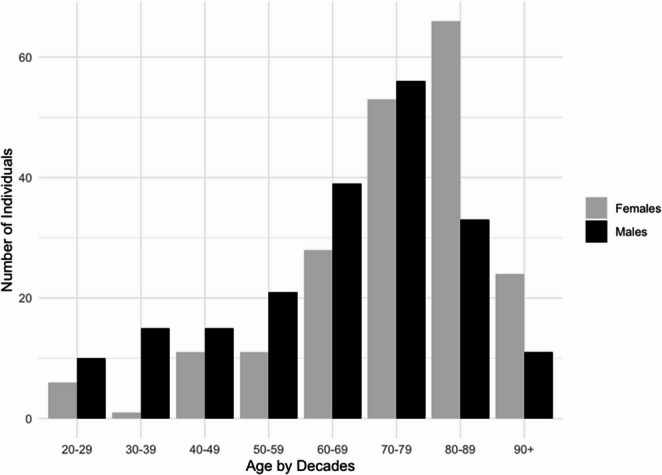 Figure 1
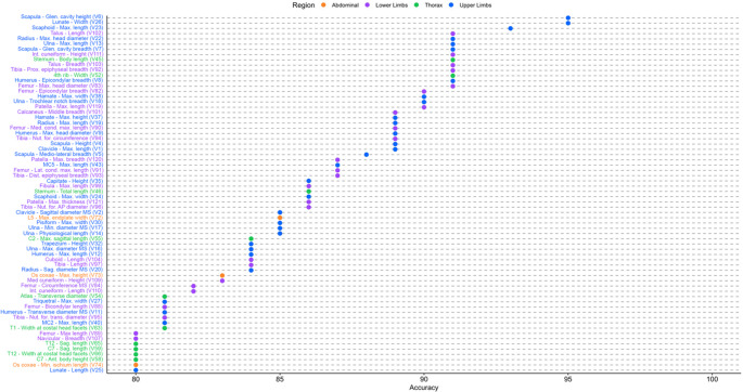 Figure 2
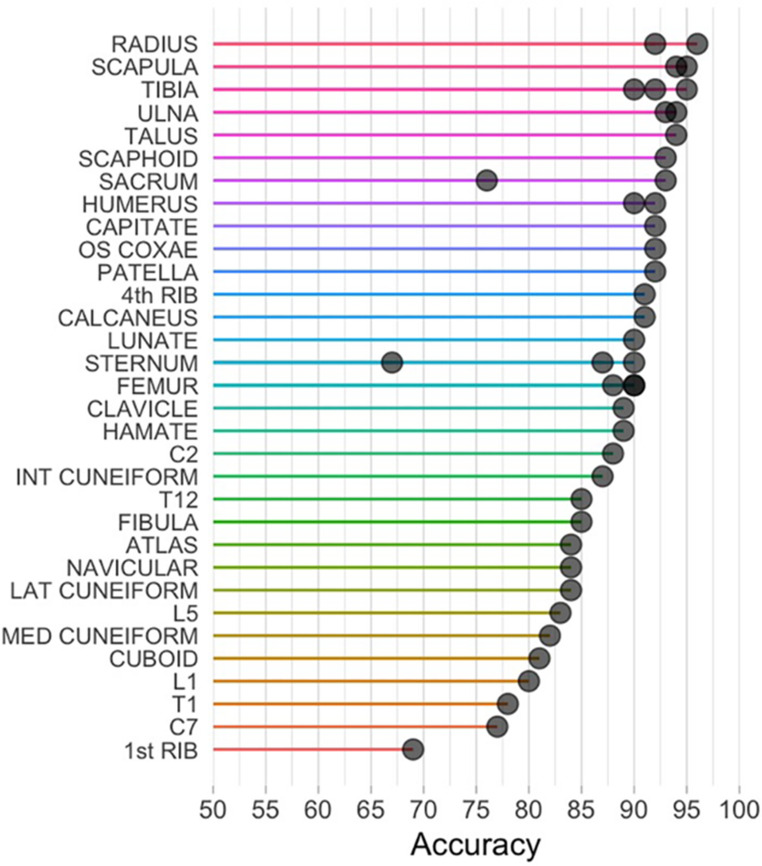 Figure 3
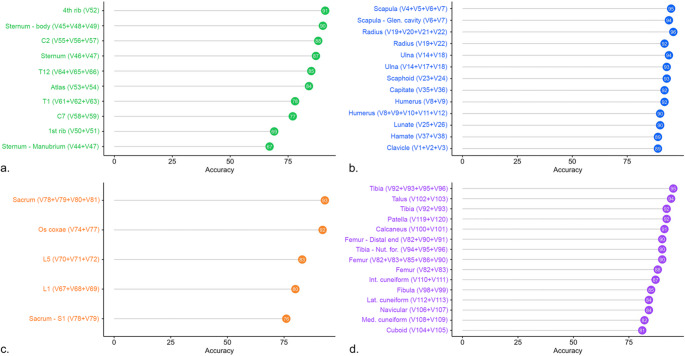 Figure 4
Peer Reviews
No public reviews on file for this paper yet. If you reviewed it on a platform where reviews are public (OpenReview, ICLR, NeurIPS, ICML), you can paste yours below so the community can read it here.
Videos
No videos yet. Explain this paper in a talk, walkthrough, or lecture? Add one.
Taxonomy
TopicsForensic Anthropology and Bioarchaeology Studies · Forensic and Genetic Research · Autopsy Techniques and Outcomes
Introduction
Estimating biological sex (understood here as estimated assigned sex at birth) is a fundamental step in anthropological studies, both in forensic and bioarchaeological contexts. The metric method stands out for its increased objectivity and higher intra- and inter-observer agreement [1, 2]. Male skeletal dimensions are on average 8–20% greater than those of females [3, 4], depending on the populations and characteristics considered, making metric traits valid for sex estimation. Particularly, from Pearson’s pioneering studies, postcranial measurements have captured the attention of anthropologists, proving to be more accurate than cranial metric and morphological methods [2]. Numerous studies have developed and refined metric methods for sex estimation based on various anatomical regions of the postcranium [2, 5, 6]. Most metric studies focus on the long bones of the upper and lower limbs, the shoulder girdle, and the pelvis—regions that frequently yield measurements with a high degree of sexual dimorphism [2, 5–12]. However, other studies have reported excellent potential for sex estimation from measurements of less commonly considered anatomical areas, such as the vertebral column [13–15], thorax [16–19], and carpal [20–22] and tarsal bones [23, 24].
A limitation of metric approaches is the interpopulation variability. Although common patterns exist in sexual dimorphism across different populations, genetic, environmental, and cultural differences can significantly influence skeletal dimensions [25, 26]. These factors result in varying dimensions and degrees of sexual dimorphism among populations necessitating the development of population-specific methods. Applying methods developed for one population to another can lead to a significant loss of accuracy [5]. Some attempts have been made to develop universally applicable methods, such as those proposed by Albanese, who argues that metric approaches can be effective across populations when certain criteria are met: the use of a strategically chosen reference sample representing diverse degrees of human variation, the application of a robust alternative statistical framework, and the identification of meaningful and reproducible combinations of sexually dimorphic measurements [27, 28]. However, it is well-established that the use of population-specific references significantly improves the accuracy of sex estimation [2, 5, 11]. Regarding the Italian population, only a few studies have provided adequate standards for certain body regions [11, 29–33], but their applicability is limited as they focus on a restricted number of skeletal elements and often rely on small sample sizes.
This paper proposes a metric approach based on the postcranial skeleton specific to the Italian population. This approach seeks to facilitate application in many different contexts by using many post-cranial regions, and mitigate the effects of preservation, which can compromise the integrity of morphologically diagnostic anatomical parts, applicable to both individual remains and contexts involving commingled remains. Univariate analyses with sectioning points as well as multivariable analyses using logistic regression and all bones are employed to enhance estimation accuracy and reveal the metric variables that lead to the highest accuracies.
Materials and methods
The sample consisted of 400 skeletons, with equal representation and distribution of the sexes (200 males and 200 females). Individuals’ ages at death ranged from 20 to 104 years, with a mean age-at-death of 66 years (standard deviation [SD] = 18; range 20–101) for males and 75 years (SD = 16; range 21–104) for females (Fig. 1). The sample originated from the Milano Cemetery Skeletal Collection, which is part of the Laboratory of Forensic Anthropology and Odontology (LABANOF) Anthropological Collection (CAL). This is a contemporary and documented osteological collection consisting of unclaimed skeletons from Milanese cemeteries [34]. The agreement between Milanese cemeteries and the LABANOF for the recovery of unclaimed skeletal remains for educational and scientific research purposes is regulated by Article 43 of the Mortuary Police Regulation (Decree of the President of the Republic No. 285 of 10/09/1990). Documentation for each individual was possible because of a collaboration with the Local Health Authority (ASL). Thus, the selected individuals have known biological sex, age-at-death, and have birth dates ranging from 1880 to 1972 and death dates from 1927 to 2001.Fig. 1. Sample distribution by biological sex and age group
In total, 121 measurements derived from 46 postcranial bones were investigated (Supplementary Material table A). Measurements were selected among the most representative and accurate according to existing literature, principally based on Langley et al. 2016 [35] and implemented to cover all post-cranial body regions. For bilateral measurements, the left side of the body was considered, with the right side measured in case the left was absent. The number of measurements taken for each skeleton was limited by its state of preservation. Consequently, if a bone was absent or if taphonomic alterations were present at the reference points, measurement was not possible. Additionally, measurements were not recorded in cases where pathological signs and bone calluses altered the original anatomical configuration. Measurements were taken using a digital caliper with a measurement precision of 0.1 mm or an osteometric board. Circumferential measurements were obtained using a flexible tape measure. All measurements were taken by the first author of the article (PM).
Statistical analyses
For the intra-observer analysis, 17 individuals were randomly selected, and measurements were collected by the author (PM) about six months after the initial data collection. For the inter-observer analysis, 15 skeletons were randomly selected, and measurements were performed by two of the authors (PM and LB-G). For these analyses, measurements were taken on both sides of the body. Intra- and inter-observer analyses involved calculating the technical error of measurement (TEM), relative TEM (rTEM) [36], and reliability coefficient (R). Acceptable values for rTEM are based on existing literature using the same measurements, with an intra-observer error set at < 1.5% and an inter-observer error at < 2.0% [37]. These thresholds were adopted to ensure stricter standards of measurement precision. However, some studies report that rTEM values up to < 5% can still be considered acceptable [e.g. 38, 39]. The reliability coefficient R measures the consistency of repeated measurements, both by the same observer (intra-observer error) and between different observers (inter-observer error). The range of R is from 0 (not reliable) to 1 (perfectly reliable). A reliability greater than 0.95 is considered acceptable in the literature [40].
Descriptive statistics were performed using Microsoft Excel^®^ and software JASP^®^ (version 0.18.3) and were calculated for each variable. Independent Student’s t-tests were used to assess differences in dimensions between male and female measurements when data were normally distributed, while Mann-Whitney U tests were applied for non-parametric data (significance at p < 0.05). Data normality was evaluated beforehand using the Shapiro-Wilk test.
The sample was randomly divided into a training subset, comprising 75% of the individuals (300 skeletons, 150 females/150 males), and a test subset, consisting of the remaining 25% of the individuals (100 skeletons, 50 females/50 males). The data partitioning was carried out using R^®^ statistical software and the caret package [41] (version 4.4.0). The training sample was used to develop the univariate sectioning points and multivariable logistic regression analyses, while the test sample was utilized to validate the derived models. The sectioning points were obtained by averaging the mean values for males and females. Measurements higher than the sectioning point are classified as male, those lower are classified as female, and values equal to the sectioning point are categorized as indeterminate. The training and testing sample were used to evaluate the performance of the sectioning points. The accuracy percentages for each measurement were calculated by dividing the correct number for each sex by the total number of individuals for that sex, and then averaging the sex-specific classification rates to generate overall classification rates. Additionally, class discrimination bias was calculated by subtracting the female correct classifications from the male correct classifications. Class discrimination bias values between − 5% and + 5% are generally recommended in forensic contexts [42].
Regarding multivariable analysis, logistic regression equations were developed bone by bone. Logistic regression models were generated on the training sample and required all individuals to have all measurements per bone, which means each bone has a different sample size dependent on measurement availability. Furthermore, for some bones, additional logistic regression models were included to also consider reliability and applicability of the selected variables. The general form of the logistic regression equation is expressed as:
p = 1/(1 + e^−Z^).
where 𝑝 represents the probability of the outcome (in this case, male or not male), ‘e’ is Euler’s constant (e ≈ 2.71828) and 𝑍 is the linear combination of the independent variables (calculated by multiplying each measurement by its corresponding coefficient and adding the intercept). The equation produces a value between 0 and 1. A result greater than 0.5 indicates a male classification, while a result below 0.5 suggests a female classification. This value also reflects the likelihood that the observed measurements correspond to a male, with the female probability being 1-𝑝. The testing set was used to validate the models generated with the training set. The accuracy rates achieved by the testing sets are used for all further interpretations and what practitioners should also report when using these methods.
Results
Intra- and inter- observer agreement
Results of the intra- and inter-observer analyses are summarized in Table 1 and include the TEM, rTEM, and the reliability coefficient (R). Regarding intra-observer error, seven measurements exhibit a rTEM > 1.5%, though the reliability coefficient indicated an almost perfect correlation for the seven measurements. In fact, all measurements were found to be acceptable according to the reliability of coefficient standards (> 0.95).Table 1. Technical error of measurement (TEM), relative technical error of measurement (rTEM) and coefficient of reliability (R) values for inter- and intra-observer error tests. N is the number of observations per test. rTEM exceeding standard thresholds are in boldBoneMeasurementIntra-observerInter-observernTEMrTEMR**nTEMrTEMRV1CLAVICLEMax. length230.5800.39%0.997160.6080.42%0.998V2CLAVICLESagittal diameter MS300.362**3.20%0.980280.4253.68%0.975V3CLAVICLEVertical diameter MS300.3183.10%0.975280.3953.89%0.945V4SCAPULAHeight240.7570.49%0.99760.2890.18%0.998V5SCAPULAMedio-lateral breadth290.3150.29%0.983140.5230.49%0.996V6SCAPULAGlen. cavity height330.3751.03%0.990190.4511.27%0.981V7SCAPULAGlen. cavity breadth320.2030.76%0.994200.4001.52%0.983V8HUMERUSEpicondylar breadth310.1360.23%1.000230.2150.36%0.998V9HUMERUSMax. head diameter270.1610.36%0.998250.2720.60%0.996V10HUMERUSSagittal diameter MS330.2731.32%0.992270.5152.49%0.972V11HUMERUSTransverse diameter MS330.3361.75%0.975270.4952.48%0.980V12HUMERUSMax. length310.2380.08%1.000240.7220.22%0.999V13ULNAMax. length230.3040.12%1.000140.6810.27%0.999V14ULNAPhysiological length260.2860.13%1.000150.4830.22%0.999V15ULNAMin. circumference260.3601.00%0.995171.4854.22%0.959V16ULNAMax. diameter MS310.1971.22%0.992190.4933.06%0.968V17ULNAMin. diameter MS310.1771.53%0.992190.4613.94%0.957V18ULNATrochlear notch breadth320.2411.21%0.992230.2801.38%0.983V19RADIUSMax. length270.3790.16%1.000160.6370.27%0.999V20RADIUSSag. diameter MS300.2061.79%0.981210.2992.61%0.963V21RADIUSTrans. diameter MS300.1601.06%0.993210.3132.09%0.980V22RADIUSMax. head diameter280.1420.65%0.996100.1320.58%0.988V23SCAPHOIDMax. length110.0830.30%0.99970.1580.61%0.998V24SCAPHOIDMax. width110.2421.47%0.98370.1771.09%0.994V25LUNATELength110.1690.96%0.99270.2751.59%0.989V26LUNATEWidth110.1760.97%0.99370.1891.10%0.995V27TRIQUETRALMax width70.2001.34%0.98920.1000.79%1.000V28TRIQUETRALMax height70.1801.12%0.99920.2241.41%1.000V29PISIFORMMax. length30.1631.05%0.99110.0000.00%-V30PISIFORMMax. width30.2242.21%1.00010.0000.00%-V31TRAPEZIUMMax. length100.0320.13%1.00050.0550.24%0.999V32TRAPEZIUMHeight100.1140.60%0.99750.1671.01%0.998V33TRAPEZOIDLength of palmar surf.100.0590.34%0.99950.1000.62%0.963V34TRAPEZOIDWidth of dorsal surf.100.1241.04%0.99650.1611.45%0.995V35CAPITATEHeight110.1930.80%0.989120.1100.47%0.999V36CAPITATEWidth of distal base110.2111.52%0.992100.2481.87%0.993V37HAMATEMax. height140.3051.28%0.98950.3191.37%0.970V38HAMATEMax. width150.1610.77%0.99760.1500.72%0.996V39MC1Max. length140.1000.21%1.000110.3500.78%0.997V40MC2Max. length170.1530.22%0.999130.3020.46%0.998V41MC3Max. length190.2180.31%0.998120.4560.71%0.992V42MC4Max. length160.1320.23%0.999130.2970.54%0.994V43MC5Max. length160.1920.35%0.999110.3340.64%0.989V44STERNUMManubrium length110.2860.57%0.99950.6151.21%0.953V45STERNUMBody length120.4230.45%0.99970.3080.32%1.000V46STERNUMTotal length80.3360.24%1.00030.9390.63%0.999V47STERNUMManubrium max. width81.3472.32%0.97540.6001.03%0.990V48STERNUMSup. body width130.1790.68%0.99970.1790.66%0.998V49STERNUMInf. Body width110.3550.98%0.99950.3631.13%0.996V501^ST^ RIBMax. chord201.0011.18%0.99181.1861.48%0.996V511^ST^ RIBMin. chord200.8951.66%0.991121.3492.54%0.985V524^TH^ RIBWidth110.1430.86%0.99930.2612.08%0.995V53ATLASSagittal diameter120.1680.36%0.99990.3550.77%0.987V54ATLASTransverse diameter110.4560.59%0.99340.1460.18%0.998V55C2Max. sagittal length90.3990.80%0.97660.5971.26%0.981V56C2Max. height100.3170.81%0.961100.4041.06%0.969V57C2Max. breadth sup. facets110.0600.13%1.000100.4601.01%0.994V58C7Ant. body height90.0820.61%0.997100.2211.62%0.991V59C7Sag. length80.1390.22%1.00080.2550.42%0.998V60C7Max width60.1160.17%1.00010.5660.76%-V61T1Ant. body height90.1551.04%0.995100.3061.96%0.991V62T1Sag. length60.2720.43%0.96650.6721.07%0.985V63T1Width at costal head facets90.2480.73%0.998100.3781.14%0.990V64T12Ant. body height150.1970.82%0.98560.1320.60%0.999V65T12Sag. length100.5460.76%0.99330.5510.72%0.999V66T12Width at costal head facets110.1020.24%1.00060.4841.12%0.989V67L1Ant. body height130.1820.71%0.99080.2511.01%0.989V68L1Sag. length80.3220.41%0.99820.4000.55%1.000V69L1Max. endplate width110.2070.45%0.99980.6051.37%0.986V70L5Ant. body height100.1920.67%0.99350.2100.74%0.996V71L5Sag. length60.1980.26%0.99950.7240.98%0.997V72L5Max. endplate width90.0710.14%1.00060.7651.56%0.977V73OS COXAEMax. heigth260.3980.19%0.999200.7910.38%0.999V74OS COXAEMin. ischium length260.4740.86%0.992170.5290.96%0.993V75OS COXAEIliac breadth180.6560.42%0.987131.2680.83%0.967V76OS COXAEMin. pubis length160.6190.86%0.991100.8301.19%0.968V77OS COXAEMax. I.P. ramus length180.8610.89%0.986141.0571.09%0.929V78SACRUMS1 trans. diameter150.5681.20%0.992110.4861.07%0.994V79SACRUMS1 sagittal diameter140.2100.67%0.996100.5181.74%0.978V80SACRUMAnterior height120.2940.28%0.99940.8980.88%0.992V81SACRUMAnterior breadth131.6151.47%0.953101.1941.11%0.979V82FEMUREpicondylar breadth290.2560.32%0.998230.3360.42%0.998V83FEMURMax. head diameter310.2090.46%0.998250.3400.74%0.994V84FEMURCircumference MS341.0071.18%0.991271.0181.17%0.986V85FEMURTrans. Diameter MS340.2691.03%0.992270.2140.82%0.992V86FEMURSagittal diameter MS340.4141.47%0.983270.3951.40%0.989V87FEMURTrans. subtroch. diameter340.4041.36%0.987270.5421.71%0.959V88FEMURBicondylar length320.5340.12%1.000260.8580.19%0.999V89FEMURMax. length320.5190.12%1.000260.8880.20%0.999V90FEMURMed. cond. max. length270.4100.66%0.996230.5090.82%0.992V91FEMURLat. cond. max. length260.2580.42%0.997250.5610.91%0.988V92TIBIAProx. epiphyseal breadth220.4110.56%0.999210.5040.69%0.995V93TIBIADist. epiphyseal breadth250.4470.99%0.991170.8751.90%0.983V94TIBIANut. for. circumference300.7750.86%0.995271.4211.55%0.984V95TIBIANut. for. trans. diameter300.3731.51%0.988270.4952.00%0.981V96TIBIANut. for. AP diameter300.4831.51%0.981270.5581.77%0.981V97TIBIALength290.4200.12%1.000250.7210.21%0.999V98FIBULAMax. diameter MS320.1631.05%0.995250.3162.13%**0.968V99FIBULAMax. length200.2370.07%1.000160.5300.15%1.000V100CALCANEUSMax. length180.3240.40%0.997170.5140.64%0.991V101CALCANEUSMiddle breadth200.3520.85%0.993200.7371.81%0.966V102TALUSLength210.1860.32%0.999230.4690.80%0.994V103TALUSBreadth210.3700.92%0.994210.3190.76%0.993V104CUBOIDLength170.1400.37%0.998180.3150.83%0.992V105CUBOIDBreadth160.2170.77%0.997140.3421.23%0.976V106NAVICULARLength190.2671.28%0.970180.4332.02%0.971V107NAVICULARBreadth190.2660.66%0.993180.3270.81%0.983V108MED CUNEIFORMLength190.1620.61%0.992170.4591.71%0.970V109MED CUNEIFORMHeight190.3260.98%0.988170.3080.94%0.988V110INT CUNEIFORMLength160.2621.39%0.972160.3411.81%0.980V111INT CUNEIFORMHeight160.1980.90%0.994130.1970.93%0.989V112LAT CUNEIFORMLength150.1080.45%0.995180.3761.50%0.964V113LAT CUNEIFORMHeight150.2110.92%0.992140.2120.93%0.976V114MT1Max. length170.3620.58%0.993100.2090.33%0.998V115MT2Max. length190.1430.19%0.999150.2890.40%0.998V116MT3Max. length170.1930.27%0.999140.2350.35%0.998V117MT4Max. length160.2030.29%0.999140.2680.40%0.999V118MT5Max. length180.2920.42%0.996110.4910.71%0.963V119PATELLAMax. length80.2770.63%0.993100.3660.90%0.988V120PATELLAMax. breadth70.1250.28%0.999100.2850.67%0.995V121PATELLAMax. thickness80.2241.08%0.983140.2441.21%0.985
Concerning inter-observer analysis, a rTEM > 2.0% was found for 13 measurements, yet like the intra-observer analyses, all measurements met the reliability coefficient standards (R > 0.95), indicating a strong association between the measurements taken by the two observers. The measurements that showed a higher-than-acceptable intra-observer error also exhibited an inter-observer error beyond the acceptable standards, with the notable exception of the maximum width of the manubrium, which only displayed an intra-observer error.
No measurement was excluded from the evaluation based on intra- and interobserver error. Moreover, although we adopted stricter thresholds regarding the rTEM (< 1.5% and < 2.0%), it is important to note that all measurements also fall within the broader limits (< 5%) considered acceptable in the literature. Nonetheless, it is recommended to exercise caution when measuring those variables that may be subject to lower reliability.
Differences between sexes
The average male measurements were found to be greater than those of females, except for three measurements: minimum pubic length, maximum ischiopubic ramus length, and anterior width of the sacrum (Table 2). Most measurements showed a significant p-value, less than 0.001, indicating a strong difference between the measurements in the two sexes. Three measurements were not statistically significant: minimum pubic length (p = 0.286), maximum ischiopubic ramus length (p = 0.101) and anterior width of the sacrum (p = 0.832). Consequently, these measurements were excluded from single variable analyses.Table 2. Results of the single variable analysis. Sectioning points (sec point), in millimeters, along with their respective accuracy and class discrimination bias (CD bias), are provided. M, F, and T indicate the number of observations for males, females, and total, respectively. NS results are non-significantBoneMeasurementTraining sampleTest sampleMFTmean Mmean Fsec pointaccuracyCD biasMFTaccuracyCD biasV1CLAVICLEMax. length11994213154.0139.0146.582.6%−6.3%32326489.1%−9.4%V2CLAVICLESagittal diameter MS13913127012.210.111.281.9%−2.6%45479285.9%−2.8%V3CLAVICLEVertical diameter MS13913026910.98.89.984.0%−1.2%45489376.3%2.8%V4SCAPULAHeight8050130159.8138.0148.984.6%−2.3%28184689.1%−8.7%V5SCAPULAMedio-lateral breadth10373176110.798.3104.588.1%−6.3%35286388.9%−7.1%V6SCAPULAGlen. cavity height14011625638.433.235.890.2%1.1%43448795.4%−4.7%V7SCAPULAGlen. cavity breadth13411625028.824.626.785.2%1.3%41438491.7%2.0%V8HUMERUSEpicondylar breadth13611725362.553.958.289.7%−3.2%42499191.2%−1.4%V9HUMERUSMax. head diameter13310824147.741.844.789.6%−2.0%45398489.3%−10.4%V10HUMERUSSagittal diameter MS14314128421.518.520.082.0%2.4%47519871.4%5.8%V11HUMERUSTransverse diameter MS14314128420.517.318.981.7%−1.2%47519881.6%2.6%V12HUMERUSMax. length133118251324.5295.8310.279.7%1.6%44458984.3%−0.4%V13ULNAMax. length10478182258.2228.3243.285.7%4.2%35256091.7%−7.4%V14ULNAPhysiological length11395208227.4202.5214.983.2%3.9%40367685.5%4.2%V15ULNAMin. circumference11210922137.832.034.980.1%2.4%36387474.3%−14.9%V16ULNAMax. diameter MS13412525916.914.015.584.2%−5.9%45459084.4%−4.4%V17ULNAMin. diameter MS13512726212.39.811.190.5%2.9%45459085.6%−15.6%V18ULNATrochlear notch breadth14012126121.117.719.484.7%−2.4%46479390.3%−6.7%V19RADIUSMax. length12098218239.7212.5226.185.8%−1.7%40367689.5%−4.2%V20RADIUSSag. diameter MS13512225712.09.911.088.7%−4.3%46489484.0%−7.1%V21RADIUSTrans. diameter MS13412626015.613.514.678.1%−2.5%45479270.7%5.2%V22RADIUSMax. head diameter1159521023.319.821.590.0%−2.9%37367391.8%−5.3%V23SCAPHOIDMax. length43418428.124.526.378.6%−8.5%10192993.1%−4.7%V24SCAPHOIDMax. width44408416.714.615.777.4%−5.0%10192986.2%−24.7%V25LUNATELength38306618.515.717.181.8%−6.8%8122080.0%−29.2%V26LUNATEWidth38306618.616.017.387.9%−8.6%8122095.0%−12.5%V27TRIQUETRALMax width20214115.513.914.782.9%−5.7%471181.8%−50.0%V28TRIQUETRALMax height19214016.914.615.885.0%−11.5%4711100.0%0.0%V29PISIFORMMax. length1081814.813.114.072.2%17.5%25771.4%40.0%V30PISIFORMMax. width981710.09.19.670.6%15.3%25785.7%20.0%V31TRAPEZIUMMax. length31255624.721.423.085.7%3.1%681478.6%−20.8%V32TRAPEZIUMHeight32245618.316.617.471.4%1.0%581384.6%−7.5%V33TRAPEZOIDLength of palmar surf.34316517.515.316.476.9%11.4%5111675.0%−21.8%V34TRAPEZOIDWidth of dorsal surf.35316611.710.611.157.6%−0.9%5111662.5%25.5%V35CAPITATEHeight554510024.121.322.782.0%3.6%10203086.7%−25.0%V36CAPITATEWidth of distal base554510014.212.113.276.0%−3.2%10182875.0%7.8%V37HAMATEMax. height33366924.520.822.689.9%2.0%6131989.5%15.4%V38HAMATEMax. width35427721.818.720.388.3%−4.8%7142190.5%−28.6%V39MC1Max. length646112546.542.044.382.4%4.0%14203476.5%−8.6%V40MC2Max. length918517669.264.166.675.6%7.4%24295381.1%−3.6%V41MC3Max. length868316968.262.765.572.2%−0.2%21284977.6%6.0%V42MC4Max. length676813558.353.655.974.1%4.1%19254477.3%−15.6%V43MC5Max. length605811854.349.852.178.0%0.7%12203287.5%−6.7%V44STERNUMManubrium length736714050.546.848.667.9%−15.8%20264678.3%−5.8%V45STERNUMBody length6659125101.683.992.880.0%3.9%24234791.5%8.9%V46STERNUMTotal length454590150.5128.2139.482.2%0.0%13162986.2%−2.9%V47STERNUMManubrium max. width615811958.151.654.872.3%−7.0%14264065.0%9.9%V48STERNUMSup. body width876315027.124.225.662.0%−10.8%28275570.9%8.3%V49STERNUMInf. Body width735813134.629.332.074.0%2.9%24244862.5%−8.3%V501^ST^ RIBMax. chord787114986.180.983.564.4%−8.8%23214472.7%−15.7%V511^ST^ RIBMin. chord827315555.753.554.656.1%10.3%25224755.3%1.5%V524^TH^ RIBWidth37316817.213.415.394.1%−4.9%17173491.2%−5.9%V53ATLASSagittal diameter909318347.143.045.074.3%−4.1%37286576.9%3.4%V54ATLASTransverse diameter635111481.473.377.481.6%−1.4%25194481.8%−13.5%V55C2Max. sagittal length675011752.047.049.581.2%9.1%23163984.6%−15.5%V56C2Max. height958818340.336.638.577.0%3.9%30235375.5%−20.3%V57C2Max. breadth sup. facets1008718747.443.845.675.4%5.6%29275673.2%−1.7%V58C7Ant. body height807315314.112.513.374.5%−4.2%27245180.4%18.1%V59C7Sag. length714611761.954.258.083.8%−1.7%22143680.6%3.2%V60C7Max width20133374.366.370.378.8%−9.6%3710100.0%0.0%V61T1Ant. body height807415416.014.115.074.7%5.9%27295675.0%26.8%V62T1Sag. length654410963.756.660.284.4%−3.3%26164278.6%15.9%V63T1Width at costal head facets847716134.230.932.671.4%−10.0%33306381.0%1.8%V64T12Ant. body height997016924.022.523.365.7%−4.9%30306063.3%0.0%V65T12Sag. length53348776.068.072.079.3%9.5%20113180.6%−15.9%V66T12Width at costal head facets1047217645.541.043.272.7%0.9%29275680.4%−9.3%V67L1Ant. body height917616725.824.325.167.7%1.0%31275858.6%−15.1%V68L1Sag. length52439580.072.576.277.9%2.1%17122979.3%−6.9%V69L1Max. endplate width897716648.043.245.675.9%−3.8%31265777.2%−20.7%V70L5Ant. body height966616228.526.827.766.7%−2.6%28265463.0%10.2%V71L5Sag. length51429377.871.274.575.3%2.7%13132673.1%7.7%V72L5Max. endplate width926215452.947.350.179.2%−15.9%28285685.7%−7.1%V73OS COXAEMax. heigth11179190215.6198.6207.178.9%−10.0%29336283.9%4.4%V74OS COXAEMin. ischium length1158219757.151.154.179.2%−12.7%34316580.0%17.3%V75OS COXAEIliac breadth6955124158.8152.5155.665.3%−0.2%23254866.7%22.3%V76OS COXAEMin. pubis length634310670.972.571.7NS------V77OS COXAEMax. I.P. ramus length694711696.898.797.8NS------V78SACRUMS1 trans. diameter1008518548.943.246.179.5%−9.7%32346675.8%4.6%V79SACRUMS1 sagittal diameter867215832.629.230.975.9%6.8%27295675.0%−8.9%V80SACRUMAnterior height7237109108.7100.2104.568.8%10.1%20183865.8%40.6%V81SACRUMAnterior breadth8567152106.3106.4106.4NS------V82FEMUREpicondylar breadth11810722583.273.078.192.0%−2.8%39377690.8%−2.1%V83FEMURMax. head diameter13512425948.042.045.086.9%−2.0%43468991.0%3.9%V84FEMURCircumference MS14012826891.380.886.182.1%0.1%48459382.8%−3.2%V85FEMURTrans. Diameter MS14312827127.725.026.472.3%−0.6%48469468.1%9.9%V86FEMURSagittal diameter MS14312927229.626.027.879.8%−1.6%48489675.0%−8.3%V87FEMURTrans. subtroch. diameter14813428232.028.630.378.0%−0.7%47489572.6%7.8%V88FEMURBicondylar length142123265446.8408.6427.779.6%−6.2%43448781.6%−0.4%V89FEMURMax. length143127270449.3411.9430.680.0%−5.1%43468980.9%1.0%V90FEMURMed. cond. max. length13511024564.457.160.884.9%0.6%43428589.4%7.3%V91FEMURLat. cond. max. length1229922164.357.961.183.7%−2.1%38407887.2%−0.7%V92TIBIAProx. epiphyseal breadth10610220877.067.072.091.8%1.3%36336991.3%6.6%V93TIBIADist. epiphyseal breadth13011324348.943.146.086.8%1.9%34367087.1%−3.6%V94TIBIANut. for. circumference14214428697.283.490.385.0%−3.7%47469389.2%−4.1%V95TIBIANut. for. trans. diameter14314428726.222.624.481.9%−4.3%47489581.1%−8.8%V96TIBIANut. for. AP diameter14214428633.928.931.484.6%−1.6%47469386.0%6.8%V97TIBIALength134127261363.2330.2346.778.5%−3.4%46428884.1%−3.1%V98FIBULAMax. diameter MS13712926614.913.214.170.7%−4.3%45438859.1%−7.2%V99FIBULAMax. length9975174361.1332.9347.077.6%0.4%28235186.3%−1.2%V100CALCANEUSMax. length1149921382.474.878.679.3%−0.9%30336379.4%7.6%V101CALCANEUSMiddle breadth11511222743.038.440.782.8%−0.4%31376889.7%13.0%V102TALUSLength12112424560.453.657.085.3%−0.4%32417391.8%3.5%V103TALUSBreadth11911123042.937.840.383.9%−1.5%31397091.4%9.6%V104CUBOIDLength10111521638.134.036.175.0%−1.4%26376384.1%7.4%V105CUBOIDBreadth869518128.825.627.280.1%4.7%19294877.1%−5.6%V106NAVICULARLength10212222421.318.820.077.7%−0.4%30376777.6%10.4%V107NAVICULARBreadth9710820540.636.638.677.6%1.5%29285780.7%11.2%V108MED CUNEIFORMLength10311922226.924.425.780.2%0.8%27376476.6%−4.3%V109MED CUNEIFORMHeight10211221433.630.532.178.5%1.7%27346183.6%2.8%V110INT CUNEIFORMLength9111320419.317.618.576.0%−2.3%21365782.5%−2.4%V111INT CUNEIFORMHeight859417922.520.121.377.1%−1.2%18294791.5%4.8%V112LAT CUNEIFORMLength9011520525.323.024.176.1%7.0%23406376.2%10.1%V113LAT CUNEIFORMHeight789917724.021.422.775.1%−3.7%19315076.0%21.7%V114MT1Max. length789417264.659.562.078.5%−0.5%20274776.6%5.9%V115MT2Max. length11010321377.371.974.676.5%−4.1%27325978.0%−0.3%V116MT3Max. length10410621072.067.069.574.3%5.2%25315675.0%−5.4%V117MT4Max. length10010020070.765.668.275.0%−2.0%24295367.9%12.9%V118MT5Max. length948718171.566.268.973.5%−0.2%22305271.2%−13.0%V119PATELLAMax. length687514343.638.040.885.3%2.8%17244190.2%−13.5%V120PATELLAMax. breadth727514745.640.142.881.6%0.6%17244187.8%−19.4%V121PATELLAMax. thickness707814821.318.820.082.4%−1.9%17264386.0%−6.1%
Single variable sex estimation: sectioning points
Table 2 shows the sectioning points calculated for each measurement, along with their respective accuracy and class discrimination bias. In the validation test, correct classification percentages range from 55.3% (minimum chord of the first rib) to 95.4% (height of the glenoid cavity of the scapula). Two measurements were able to correctly classify all individuals (100%): maximum height of the triquetral and maximum width of C7. However, these two measurements were tested on only 11 and 10 individuals, respectively, a number too small for the result to be considered valid. Excluding measurements with an insufficient sample size, the variable that shows the highest accuracy is the height of the glenoid cavity of the scapula, with an accuracy of 95.4% and a class discrimination bias of −4.7% (Table 2; Fig. 2). In the training sample, the measurement with the highest classification rate was the width of the fourth rib (94.1%; class discrimination bias − 4.9%), although this result decreased slightly in the validation test (91.2%; class discrimination bias − 5.9%). In total, eighteen measurements resulted in correct classifications greater than 90% in the validation test, including measurements from the scapula, long bones of the upper limb, scaphoid, lunate, hamate, sternum, femur, tibia, patella, talus and intermediate cuneiform (Table 2; Fig. 2). Furthermore, a total of 66 measurements, across all post-cranial body regions, reported an accuracy greater than 80% (Fig. 2).Fig. 2. Visualization of sectioning point accuracies (showing only those with an accuracy greater than 80%), arranged from highest to lowest accuracy in the test sample. Measurements are color-coded by anatomical region, as indicated in the legend
Multivariable analysis
Multivariable logistic regression models were developed for each bone. In total, 43 logistic regression models were developed for 32 bones. The models and their corresponding coefficients are reported in Table 3. Table 4 summarizes the results of the models and validity tests. Correct classifications in the test set ranged from 67.6 to 96.8% (Table 4). The manubrium (67.6%; class discrimination bias − 17.7%) and first rib (69.3%; class discrimination bias 15.9%) performed the worst and the radius (96.8%; class discrimination bias 6.0%), scapula (95.3%; class discrimination bias 7.4%), and tibia (95.2%; class discrimination bias − 3.6%) performed the best (Fig. 3). Even with the lower accuracies reported for the manubrium and first rib, total accuracy rates exceeding or approaching 90% were achieved for all body regions (Fig. 4).Table 3. Coefficients for logistic models. To use these algorithms. Multiply each measurement (in millimeters) by its respective coefficient, sum the results, and add the intercept. Predicted probabilities greater than 0.5 are more likely to be males, while values below 0.5 are more likely to be females. Use table 4 for the performance metrics associated with each modelBoneMeasurementsIntercept1CLAVICLEMax length (0.186) + sagittal diameter MS (0.594) + vertical diameter MS (1.824)−51.4422SCAPULAHeight (0.076) + medio-lateral breadth (0.090) + Glen. cavity height (0.820) + Glen. cavity breadth (0.301)−57.4273SCAPULA (glenoid cavity)Glen. cavity height (0.968) + glen. cavity breadth (0.432)−45.9314HUMERUSEpicondylar breadth (0.314) + Max head diameter (0.718)−49.8895HUMERUSEpicondylar breadth (0.301) + max head diameter (0.678) + sag. diameter MS (−0.092) + trans. diameter MS (0.160) + max length (0.007)−50.5966ULNAPhys. length (0.098) + min diameter MS (0.858) + trochlear notch breadth (0.682)−43.6027ULNAPhys. length (0.118) + trochlear notch breadth (0.848)−41.3438RADIUSMax length (0.139) + sag. diameter MS (3.117) + trans. diameter MS (−0.711) + max head diameter (1.821)−93.3639RADIUSMax length (0.125) + max head diameter (1.941)−69.33410SCAPHOIDMax length (0.569) + max width (1.072)−31.47911LUNATELength (0.803) + Width (1.192)−33.98912CAPITATEHeight (1.226) + width of distal base (0.683)−36.52513HAMATEMax height (2.000) + max width (0.574)−56.82214STERNUMTotal length (0.151) + manubrium width (0.171)−30.25315STERNUM (manubrium)Manubrium length (0.055) + manubrium width (0.270)−17.37816STERNUM (body)Body length (0.146) + sup. body width (0.128) + inf. body length (0.066)−18.83417 1 st RIBMax chord (0.099)−8.189184th RIBWidth (1.588)−24.06719ATLASSag. diameter (0.347) + trans. diameter (0.344)−42.06620C2Max sag. length (0.512) + max height (0.050) max breadth sup. facets (0.215)−36.85321C7Ant. body height (0.366) + sag. length (0.418)−28.78622T1Ant. body height (0.601) + sag. length (0.308) + width at costal head facets (0.271)−35.98023T12Ant. body height (0.315) + sag. length (0.205) + width at costal head facets (0.274)−33.05424L1Ant. body height (0.128) + sag. length (0.134) + max endplate width (0.214)−23.02925L5Ant. body height (0.447) + sag. length (0.021) + max endplate width (0.547)−40.81826OS COXAEMin ischium length (1.636) + Max ramus I-P length (−0.640)−24.82627SACRUMS1 trans. diameter (0.418) + S1 sag. diameter (0.254) + anterior height (0.065) + anterior breadth (−0.187)−13.05328SACRUM (S1)S1 transverse diameter (0.191) + S1 AP diameter (0.378)−20.17929FEMUREpicondylar breadth (0.501) + max head diameter (0.351) + trans. diameter MS (−0.251) + AP diameter MS (0.231) + max length (0.040)−56.77330FEMUREpicondylar breadth (0.530) + max head diameter (0.328)−55.89231FEMUR (distal end)Epicondylar breadth (0.680) + med.cond. max length (0.279) + lat.cond. max length (−0.037)−67.30132TIBIAProx epiphyseal breadth (0.522) + Dist epiphyseal breadth (0.373) +for.nut. trans diameter (−0.452) + for.nut. AP diameter (0.480)−58.44633TIBIAProx epiphyseal breadth (0.596) + Dist epiphyseal breadth (0.298)−56.33334TIBIA (nutrient foramen)Nut. for. circum. (0.082) + nut.for. trans diameter (0.195) + nut.for. AP diameter (0.507)−27.93735FIBULAMax diameter MS (0.218) + max length (0.062)−24.36836CALCANEUSMax length (0.225) + middle breadth (0.490)−37.43337TALUSLength (0.404) + breadth (0.422)−39.91638CUBOIDLength (0.283) + breadth (0.647)−27.94439NAVICULARLength (0.549) + breadth (0.416)−27.08840MED CUNEIFORMLength (0.636) + height (0.465)−31.34341INT CUNEIFORMLength (0.483) + height (0.662)−23.11042LAT CUNEIFORMLength (0.669) + height (0.560)−29.06743PATELLAMax length (0.419) + max breadth (0.432)−35.530Table 4Accuracies (%t = overall, %M = male correct classification, %F = female correct classification) and class discrimination bias (CD bias) of the multivariable logistic regression models. Refer back to table 2 for variables and to table 3 for respective logistic regression modelsBoneMeasurementsTraining sampleTest samplen%T%M%FCD biasn%T%M%FCD bias1CLAVICLEV1 + V2 + V321193.8%93.6%94.1%−0.5%6489.1%87.5%90.6%−3.1%2SCAPULAV4 + V5 + V6 + V712294.3%93.3%94.8%−1.5%4295.3%100.0%92.6%7.4%3SCAPULA (glenoid cavity)V6 + V724591.0%92.0%90.2%1.8%8394.0%93.0%95.0%−2.0%4HUMERUSV8 + V920991.9%89.8%93.4%−3.6%7792.2%94.6%90.0%4.6%5HUMERUSV8 + V9 + V10 + V11 + V1220692.2%90.9%93.2%−2.3%7790.9%91.9%90.0%1.9%6ULNAV14 + V17 + V1819491.2%89.5%92.6%−3.1%7493.2%97.1%90.0%7.1%7ULNAV14 + V1819888.4%87.2%89.3%−2.1%7594.7%97.1%92.5%4.6%8RADIUSV19 + V20 + V21 + V2217596.6%96.0%97.0%−1.0%6296.8%100.0%94.0%6.0%9RADIUSV19 + V2218493.5%92.5%94.2%−1.7%6492.2%90.0%94.1%−4.1%10SCAPHOIDV23 + V248385.6%87.5%83.7%3.8%2993.1%94.7%90.0%4.7%11LUNATEV25 + V266687.9%85.7%89.5%−3.8%2090.0%100.0%75.0%25.0%12CAPITATEV35 + V3610088.0%86.7%89.1%−2.4%2892.9%94.4%90.0%4.4%13HAMATEV37 + V386991.3%91.7%90.9%0.8%2089.5%84.6%100.0%−15.4%14STERNUMV46 + V477588.0%86.8%89.2%−2.4%2487.5%76.9%100.0%−23.1%15STERNUM (manubrium)V44 + V4711670.7%71.9%69.5%2.4%3767.6%60.9%78.6%−17.7%16STERNUM (body)V45 + V48 + V4910880.6%78.0%82.8%−4.8%4490.9%95.2%87.0%8.2%17 1 st RIBV50 + V5113863.0%62.1%63.9%−1.8%3969.3%77.8%61.9%15.9%184th RIBV526894.1%96.8%91.9%4.9%3491.2%94.1%88.2%5.9%19ATLASV53 + V5411085.5%82.0%88.3%−6.3%4484.1%84.2%84.0%0.2%20C2V55 + V56 + V5710978.9%71.1%84.4%−13.3%3588.6%92.9%85.7%7.2%21C7V58 + V5911084.6%80.4%87.5%−7.1%3577.1%64.3%85.7%−21.4%22T1V61 + V62 + V6310786.0%84.1%87.3%−3.2%3778.4%57.1%91.3%−34.2%23T12V64 + V65 + V667578.7%69.2%83.7%−14.5%2785.2%90.0%82.4%7.6%24L1V67 + V68 + V698078.8%75.7%81.4%−5.7%2680.8%90.0%75.0%15.0%25L5V70 + V71 + V729084.4%82.5%86.0%−3.5%3483.3%83.3%83.3%0.0%26OS COXAEV74 + V7711095.5%92.7%97.1%−4.4%2792.6%83.3%100.0%−16.7%27SACRUMV78 + V79 + V80 + V818186.4%70.8%93.0%−22.2%3193.6%86.7%100.0%−13.3%28SACRUM (S1)V78 + V7915480.5%75.4%84.7%−9.3%5676.8%69.0%85.2%−16.2%29FEMURV82 + V83 + V85 + V86 + V9018691.9%90.1%93.3%−3.2%6590.8%89.7%91.7%−2.0%30FEMURV82 + V8321391.6%91.9%92.0%−0.1%7088.6%87.9%89.2%−1.3%31FEMUR (distal end)V82 + V90 + V9118892.6%91.6%93.3%−1.7%7190.2%88.6%91.7%−3.1%32TIBIAV92 + V93 + V95 + V9618893.1%93.3%92.9%0.4%6295.2%93.3%96.9%−3.6%33TIBIAV92 + V9319292.2%92.3%92.1%0.2%6492.2%87.5%96.9%−9.4%34TIBIA (nutrient foramen)V94 + V95 + V9628686.0%86.1%85.9%0.2%9390.3%91.3%89.4%1.9%35FIBULAV98 + V9917276.7%71.6%80.6%−9.0%4985.7%77.3%92.6%−15.3%36CALCANEUSV100 + V10120983.3%79.2%86.7%−7.5%6191.8%84.4%100.0%−15.6%37TALUSV102 + V10323087.8%86.5%89.1%−2.6%7094.3%89.7%100.0%−10.3%38CUBOIDV104 + V10518179.0%80.0%77.9%2.1%4881.3%82.8%79.0%3.8%39NAVICULARV106 + V10720477.6%79.4%75.3%4.1%5784.2%75.0%93.1%−18.1%40MED CUNEIFORMV108 + V10921480.8%82.1%79.4%2.7%6182.0%79.4%85.2%−5.8%41INT CUNEIFORMV110 + V11117980.5%81.9%78.8%3.1%4787.2%89.7%83.3%6.4%42LAT CUNEIFORMV112 + V11317681.8%84.9%77.9%7.0%5084.0%80.7%89.5%−8.8%43PATELLAV119 + V12014185.8%89.0%82.4%6.6%4192.3%95.8%88.2%7.6%n number of individuals, %T percentage of accuracy in the total sample, %M percentage of accuracy in the male sample, %F percentage of accuracy in the female sampleFig. 3Visualization of the accuracy of multivariable models, with bones ordered by accuracy. Black dots represent the multivariable logistic regression model for each boneFig. 4Visualization of the accuracy of multivariable models, divided by anatomical region (a = thorax; b = upper limb; c = abdominal; d = lower limb)
A logistic regression model was also developed for the fourth rib, even though the study considered only a single metric variable for this bone (the width of the sternal end). The logistic regression results confirm the utility found with the application of the sectioning point and provides the posterior probability. In contrast, no logistic regression models were developed for the metacarpals and metatarsals, as only a single measurement was examined for these bones, and the resulting accuracies rates from the sectioning points were insufficient to investigate further with logistic regression analysis.
Overall, the logistic regression models reported class discrimination bias values within acceptable thresholds in both the training and test samples (Table 4). Notably, the models for the radius and scapula, which demonstrated the highest classification accuracies, exhibited class discrimination bias values slightly above the recommended threshold in the test sample (6.0% and 7.4%, respectively). However, these deviations were minimal, and the corresponding models in the training sample remained within acceptable limits. There are exceptions in which models exhibited high class discrimination bias in the test sample, despite having balanced and acceptable class discrimination bias values in the training sample. These cases generally correspond to models developed with a smaller number of individuals, such as those for certain carpal bones (lunate and hamate) and vertebrae (C2, C7, T1, T12, L1).
Discussion
This study developed an easily applied and statistically substantiated method for biological sex estimation specific to the Italian population, employing both simple and multivariable metric analyses of postcranial bones. Total correct classifications in both types of models but especially in the multivariable models, were greater than 90% indicating its efficacy. Because of this high performance across the entire body, the metric analysis of postcranial elements is considered second only to the evaluation of the morphological features of the pelvis, while demonstrating better validity than both metric and non-metric features of the skull [2].
Intra- and inter- observer agreement
One of the aspects that makes the metric approach appealing is its objectivity and repeatability [43, 44]. However, defining and identifying the anatomical landmarks required for the measurements is not always straightforward, leading to a potential limitation in the reliability of the measurements. Demonstrating the complexity of identifying anatomical landmarks, some measurements of this study showed rTEM values exceeding the standard acceptability thresholds for intraobserver (rTEM > 1.5%) and interobserver (rTEM > 2.0%) error. Most of these measurements relate to the diameters at the midshaft of long bones, which is unsurprising based on previous literature that highlights these measurements as the most susceptible to measurement errors [37]. Consequently, a recent study by Langley and colleagues (2018) [37], focused on the quantification of osteometric error, suggested replacing the traditional measurement of diameters, which depend on position (i.e., transverse diameter, sagittal diameter), with minimum and maximum diameters, as these showed lower rTEM values. The present study still considered the traditional measurement of diameters, except for the ulna. However, the results of this study revealed a significant exception to the conclusions of Langley and colleagues (2018) [37]. Contrary to their prediction, the minimum and maximum diameters of the ulna, used in accordance with their recommendations, exhibited higher rTEM values than the traditional transverse and anteroposterior diameters considered for other long bones of the limbs. Another possibility is that smaller measurements may yield greater negative outcomes in TEM values. However, measurements of the carpal bones, despite their small size, did not exhibit rTEM values beyond the thresholds of acceptability, highlighting the high reliability of these measurements. This result suggests that the error associated with the measurements of the diameters may be intrinsic and not influenced by the methodological approach used, highlighting the need for further research to fully understand the causes of this discrepancy and to improve the precision of osteometric measurements.
Despite some measurements exhibiting rTEM values above the stricter thresholds adopted in this study (< 1.5% for intra-observer and < 2.0% for inter-observer error), all values remained below the broader acceptability limit of < 5% reported in the literature. Furthermore, the calculation of the reliability coefficient indicates that all measurements meet the standard threshold value (R > 0.95) [40], indicating strong agreement between measurement repetitions. The differential findings between the repeatability methods highlight how different methodological approaches can lead to different conclusions.
Differences between sexes
The Italian sample showed strong sexual dimorphism in size, demonstrated by the majority of measurements exhibiting significant differences between males and females, which is also reflected in the accuracies achieved by the sectioning points (Table 2). The results of the current study (Table 2) match or exceed those reported in the literature for other populations [2, 5, 6, 45, 46]. Contrary to most measurements, minimum pubic length, maximum ischiopubic ramus length, and anterior width of the sacrum showed greater dimensions in females. This was expected due to the adaptation of the female pelvis for childbirth, which results in longer pubic lengths and a more lateral growth of the ischiopubic ramus [47, 48]. Consistent with previous research, joint measurements are the best indicators for sex estimation based on their high accuracies, while measurements of the maximum length of long bones and midshaft diameters have less utility based on their lower accuracies, although they still provide good classification rates [2, 7, 27]. Indeed, the literature highlights that sexual dimorphism is more pronounced for body weight than for stature, with a sexual dimorphism approximately of 18% for body mass, while only 8% for stature [49]. Joint dimensions are therefore particularly dimorphic, as these areas are correlated with body weight load and muscle attachment, with males tending to have larger and more robust joints to support greater muscle mass and physical strength [50].
Single variable and multivariable analyses
Given the high level of sexual dimorphism of the Italian sample and the ability for metric data to collect precise information, the sectioning point results were excellent in terms of accuracy. This extremely simple approach, was capable of achieving accuracies over 80% for all body regions, and even 90% for some skeletal elements, such as the scapula, long bones of the upper limb, femur, tibia, sternum, fourth rib, talus, scaphoid and lunate. The application of sectioning points has the advantage of being computationally simple, quick, and can be used in a variety of biological anthropology contexts because it only requires a single variable. Therefore, this approach can also be used on fragmentary skeletal elements. The results of the multivariable analysis generally showed an improvement in accuracy compared to single variable analysis, which is also expected based on previous literature [e.g. 2, 51–55]. For each logistic regression model, the correct classification rate obtained from the test sample reported, in all body regions, was close to or exceeded 90%. The fact that the entire post-cranial skeleton exhibits comparable levels of sexual dimorphism when considered through a multivariable lens is truly remarkable. Unlike morphological methods, which are typically limited to specific sexually dimorphic traits in the pelvis and skull, the metric approach offers the advantage of providing accurate sex estimations across all post-cranial regions. This highlights a key strength of the metric approach in direct contrast to the most popular morphological approaches for sex estimation: its applicability in various conservation contexts, including commingled or fragmentary remains, regardless of the number or type of elements preserved.
Performance based on skeletal elements and variables
The scapula emerged as one of the most sexually dimorphic bones in the Italian population, with classification rates exceeding 95% in both single variable analysis and multivariable models. The glenoid cavity was the variable achieving the highest accuracy (95.4%, class discrimination bias − 4.7%) across all measurements in this study. This contrasts with findings from other populations, where maximum scapular height was often the most accurate measurement [e.g. 8, 56–59]. The glenoid cavity also showed better resistance to taphonomic changes, while the scapular body was more prone to postmortem fractures, making it a suitable area. This study’s results for multivariable scapula model (95.3%) surpass previous findings for the Italian population of 92.6% [60] and 95% accuracy [32]. Multivariable analysis of the scapula proved to be an accurate method for sex estimation in various populations, with several studies reporting accuracies over 90% [2, 8, 58, 60–64]. Similarly, Spradley et al. (2015) [6] found 95.6% accuracy in a Hispanic sample, and Moore et al. (2016) [5] reported 93.5% accuracy in a Colombian sample, confirming the consistency of the scapula’s predictive ability for sex estimation.
The long bones of the upper limb have also proven to be particularly accurate for sex estimation using metric approaches. The radius achieved the highest accuracy levels in multivariable analysis, reporting a validity of 96.8% (class discrimination bias 6%) for the equation that combines all four analyzed variables. The results align with findings from other population contexts, with accuracies consistently over 90% [2, 5, 6, 9, 12, 65–68]. Similarly to our study, Spradley and Jantz (2011) [2] found that the radius was the skeletal element providing the highest accuracy in multivariable analysis in an African American sample. In contrast, the radius had a slightly lower accuracy of 85.6% for the White American sample [2]. Likewise, in similar studies, the accuracy of multivariable analysis for the radius was around 90% for Colombian [5] and Hispanic [6] samples. However, these cited studies did not consider the metric analysis of the radial head. In the current study, the radial head measurements was the variable with the most utility in a single variable approach (91.8%) and the most significant in the multivariable logistic regression models. Previously published findings using an American sample also demonstrated the radial head could achieve high accuracies (94%) [69], as well as in a Portuguese sample (90.4%) [70] and a Thai sample (92%) [71]. Regarding the humerus, the best metric variable found was the epicondylar width, which showed better validity than the humeral head in terms of classification rate (91.2% vs. 89.3%, respectively) and class discrimination bias (−1.4% vs. −10.4%, respectively). This result contrasts with previous reports for the CAL cemetery collection, where a similar result was reported for the diameter of the humeral head, but a much lower accuracy was achieved (81.6%) for the epicondylar width [7]. The current study had a much larger sample (400 individuals vs. 164 individuals) compared to Selliah and colleagues (2020) [7], allowing for greater variability. Additionally, the comparable performance in the training and testing sets in the current study validate its performance. The ulna represented an exception among long bones, as it is the only one reporting better validity in single variable analysis for maximum length (91.7%), although it shows a class discrimination bias slightly over the recommended standards (−7.4%). Our results align with other studies that identify the maximum length of the ulna as the most accurate measurement for this bone across different populations [2, 5, 6]. Additionally, the current study introduced the measurement of the trochlear notch breadth, a rarely investigated area in osteometric studies. The research by Zapico and Adserias-Garriga (2021) [72] indicated this area as extremely valid, with an accuracy of 91.3% for the minimum olecranon breadth (similar to the trochlear notch breadth though not identical) in a small sample of European Americans. The current study highlights the validity of this new measurement, showing it can correctly discriminate between sexes in 90.3% of cases and is a significant variable in the ulna’s multivariable analysis.
The long bones of the lower limb, particularly the femur and tibia, have also proven to be particularly accurate in our study. In the multivariable analysis, the bone models exceed 90% accuracy, and reach 95.2% (class discrimination bias − 3.6%) for the tibia model, which combines epiphyseal widths and diameters measured at the nutrient foramen. The femur and tibia have been extensively studied using metric approaches, reporting high accuracies across various population contexts [e.g. 2, 5, 6, 11, 73–77]. A particularly dimorphic skeletal portion is related to the knee joint. The femoral epicondylar width and the proximal tibial , epiphyseal width achieved accuracies over 90%, with class discrimination bias contained within recommended thresholds, in single variable analysis. These measurements are reported to be the most suitable in White American and Black American populations [2], and have also shown accuracies greater than 90% in various European populations [e.g., 11, 78, 79]. The strong sexual dimorphism in this skeletal area is attributed to the knee region’s correlation with body weight load and muscle attachment [50]. Consequently, the patella also allows for effective sex estimation. In this study, single variable analysis of three metric dimensions of the patella yielded an accuracy of up to 91%, improving to 92.3% with multivariable analysis, confirming its validity for sex estimation through metric approaches [80–86].
In contrast, some skeletal elements revealed lower validity for metric sex estimation. The fibula emerged as the least sexually dimorphic long bone, as previously indicated by the literature [2, 5, 6, 39]. The first rib showed low accuracies (below 70%) with both sectioning points and multivariable analyses. This result contrasts with a Polish study that reported an accuracy of up to 90% [87]. However, the original study evaluated nine metric characteristics, while the present study considers only two. The vertebral column was the only body region where accuracy did not exceed 90%, although the multivariable analysis improved accuracy for all considered vertebrae, with validity ranging from 77.1% for C7 to 88.6% for C2. However, some studies indicate that surpassing 90% accuracy is possible for different vertebrae in various populations, often utilizing more metric variables than those selected for this study [14, 15, 88–92]. Pelvic measurements were not particularly useful for sex estimation with single variables, with the highest classification rate for the height of the os coxae at 83.9% and no sacral measurement exceeding 75%, consistent with the literature [93–95]. Even if multivariable models considerably improved the accuracy for these bones, achieving 92% accuracy for the os coxae and 93% for the sacrum, they still exhibited class discrimination bias beyond the threshold recommended for forensic applications, which could potentially compromise the validity of the estimations. The maximum length of the metacarpals and metatarsals demonstrated limited sexual dimorphism in the Italian population, with the highest accuracy of 87.5% for the fifth metacarpal and 78.2% for the second metatarsal. These results are consistent with previous studies indicating that single-variable length measurements of these bones rarely exceed 80% accuracy [96–103].
Other skeletal elements have proven valid for sex estimation but are limited in applicability due to greater susceptibility to taphonomic alterations, thus resulting in smaller sample sizes for our study. This is particularly evident for the carpal bones, for which the sample size was extremely limited due to the difficulty of recovering these small bones in this cemetery burial context [34]. The osteometric study of carpals for sex estimation has only been considered since 2008, with the pioneering research by Sulzmann et al. (2008) [20]. The current study further supports the potential of these small hand bones, reaching accuracies of up to 93%, in line with findings from other populations [20, 22, 104, 105]. Another example is the thoracic area, with the sternum and the fourth rib. The width at the sternal end of the fourth rib has also shown high classification rates in other populations [16, 19, 106, 107]. It is known that the thoracic cavity volume is about 10% smaller in females than in males of the same stature [108], which can explain the observed sexual dimorphism. Yet, it is particularly susceptible to taphonomic alterations, as the central thoracic ribs (fourth to tenth) are more prone to post-mortem fractures and environmental factors [109, 110], resulting in a limited number of individuals in the sample (68 in the training sample and 34 in the test sample). Additionally, its dimensions appear to be influenced by the individual’s age, showing an increasing trend with age [107, 111]. Given that our sample contains many older individuals, the sectioning point obtained should be applied cautiously, and future validation is necessary in younger individuals.,
Limitations
Despite the robustness of the methodology and the relatively large sample size, this study has certain limitations that should be acknowledged. The main one is related to the preservation of skeletal remains. Although the overall sample size is substantial, taphonomic alterations have affected the completeness of certain bones, reducing data availability. As a result, some anatomical regions of the skeleton are underrepresented in the analysis, such as the carpal bones and vertebral column, which potentially impacts the accuracy and generalizability of the sex estimation models for these bones. Another limitation concerns the population-specificity of the developed method. While this study focuses on a Northern Italian population, it is important to consider the regional variability that may exist within Italy itself. Factors such as geographical diversity, historical migrations, and genetic variability may affect the generalizability of these results across the entire Italian population. Therefore, while the methodology shows high accuracy for the sample analyzed, and the testing set provides a form of validation, further research is needed to assess whether it can be generalized and applied on a greater scale across Italy.
Conclusion
The collected data enabled the development and validation of a metric method for sex estimation specific to the Italian population. Whereas some components of the biological profile are not substantially impacted by population variation [e.g., 112, 113] metric data are impacted by population variation. Therefore, the current research provides a notable achievement for forensic anthropology in Italy, as it provides easy to apply yet computationally robust single variable and multivariable models to estimate sex. Up to this point, sex estimation was explored primarily in smaller samples [e.g., 7, 30] and/or only using a limited number of variables or elements [e.g., 29, 32, 33, 60, 114, 115] on Italian individuals, and when in a situation where a model was not possible, there was reliance on standards developed in other countries. Since sectioning points and their classification rates were provided for all standard postcranial measurements, and multivariable analysis was conducted on a bone-by-bone basis, the developed methodology is also applicable in contexts of commingled remains and fragmented skeletal remains.
The results presented in this study highlight the high accuracy of the metric approach for sex estimation and contribute to the growing literature illustrating the advantages of using multiple variables to increase confidence in our estimations. Multivariable logistic regression models displayed accuracies above or close to 90% with a contained class discrimination bias across all skeletal regions. The sectioning points developed allowed for an equally accurate and quick estimation of biological sex, as evidenced by 18 measurements exceeding 90% accuracy in the validation test. The models presented in the current study do not require any software or specialized training, allowing for immediate adoption by forensic laboratories across the country. We believe the large sample size adequately captures the range of human variation, and the testing sample acts as a strong validation set, however we encourage colleagues to test the developed models with additional external samples to ensure generalizability.
Supplementary Information
Below is the link to the electronic supplementary material.
Supplementary Material 1
The reference list from the paper itself. Each links out to its DOI / PubMed record.
- 1Navsa N, Iscan MY, Steyn M (2008) Sex determination from the metacarpals in a modern South African male and female sample. Poster presented at the University of Pretoria Health Sciences Faculty Day, August 2008, Pretoria, South Africa. URI: http://hdl.handle.net/2263/7406