Deterministic modelling of asymptomatic spread and disease stage progression in vaccine preventable infectious diseases
Gabor Kiss, Salissou Moutari, Cara Mctaggart, Lynsey Patterson, Frank Kee, Felicity Lamrock

TL;DR
This paper presents a model to track how vaccine-preventable diseases spread silently and progress through different stages, using a diphtheria outbreak in Yemen as an example.
Contribution
The study introduces a deterministic model for asymptomatic spread and disease progression in vaccine-preventable diseases.
Findings
The basic reproduction number increases with higher transmission rates.
The basic reproduction number decreases with higher vaccination rates.
Abstract
This study introduces a deterministic formulation for modelling the asymptotic spread of a vaccine preventable disease as well as the different stages for the progression of the disease. We derive the formula for the associated basic reproduction number. To illustrate the proposed model, we use data from the 2017–2018 diphtheria outbreak in Yemen and fit the parameters of the model. A sensitivity analysis of the basic reproduction number, with respect to the model parameters, show that this number increases with an increase of the transmission rate while this number decreases when vaccination rate increases.
Genes, proteins, chemicals, diseases, species, mutations and cell lines named across the full text — each resolved to its canonical identifier and authoritative record.
Click any figure to enlarge with its caption.
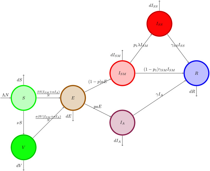 FIGURE 1
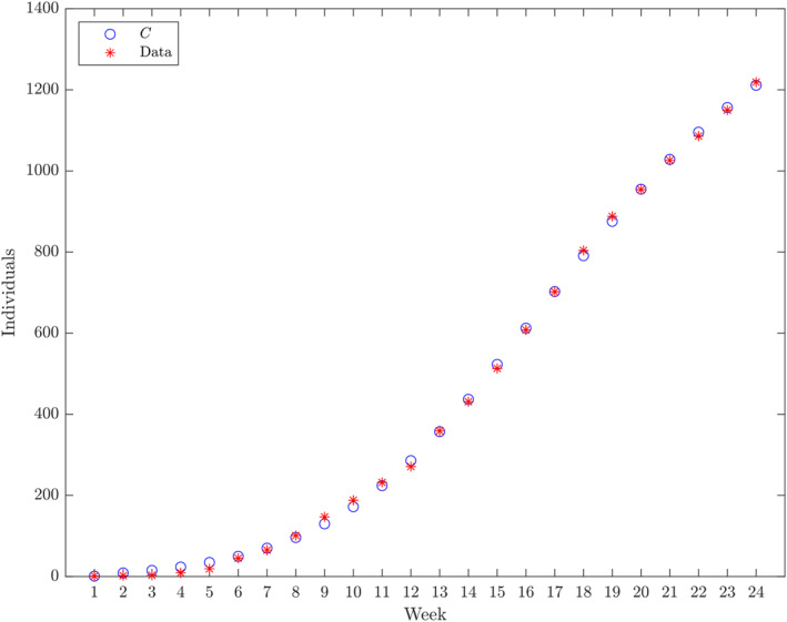 FIGURE 2
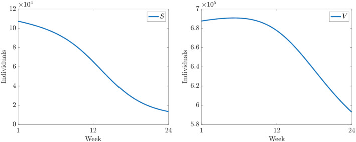 FIGURE 3
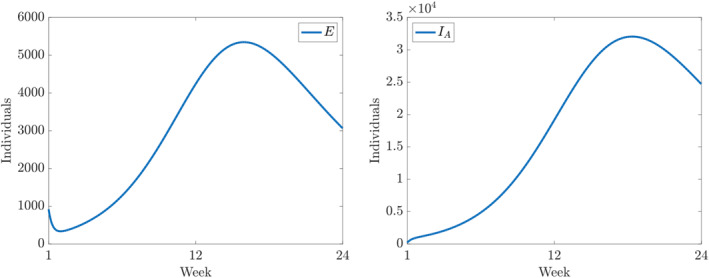 FIGURE 4
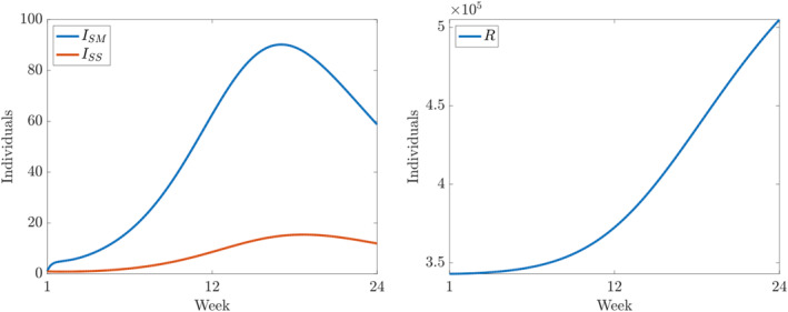 FIGURE 5
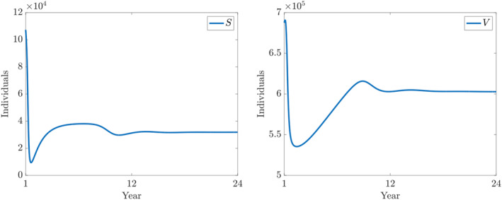 FIGURE 6
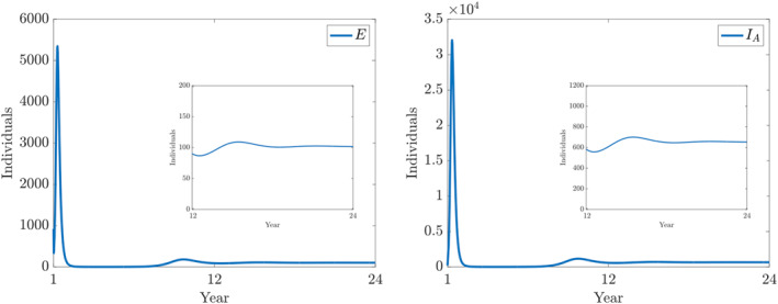 FIGURE 7
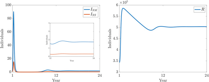 FIGURE 8
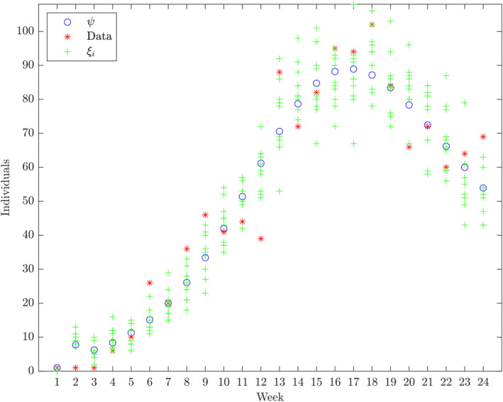 FIGURE 9
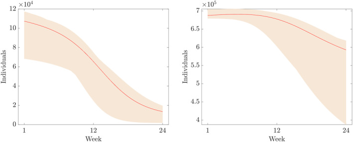 FIGURE 10
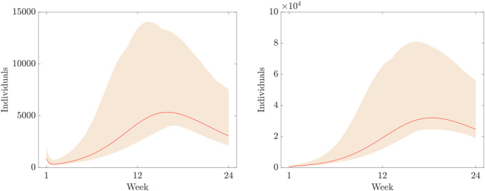 FIGURE 11
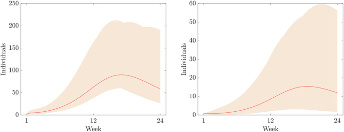 FIGURE 12
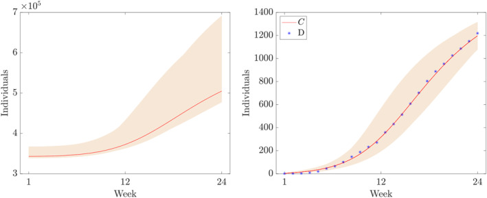 FIGURE 13
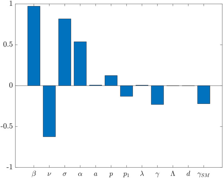 FIGURE 14
| Variable | Meaning |
|---|---|
|
| The number of susceptible individuals at time |
|
| The number of vaccinated individuals at time |
|
| The number of exposed individuals at time |
|
| The number of asymptomatically infective individuals at time |
|
| The number of infective individuals with mild symptoms at time |
|
| The number of infected individuals with severe symptoms at time |
|
| The number of recovered individuals at time |
| Parameter | Description | Range | Refs |
|---|---|---|---|
|
| Transmission rate (d−1) | 0.01–1 | ‐ |
|
| Vaccination rate (d−1) | [ | |
|
| Transmission rate reduction in vaccinated | 0.01–0.1 | [ |
|
| Infectiousness reduction in asymptomatic | 0.59–0.87 | [ |
|
| Average incubation period (d) | 2–5 | [ |
|
| Probability of being asymptomatic | 0.83–1 | ‐ |
|
| Probability of developing severe symptoms | 0.1–0.25 | [ |
|
| Time to develop severe symptoms (d) | 7–14 | [ |
|
| Asymptomatic infectious period (d) | 17–20 | [ |
| Mild symptomatic infectious period (d) | 5–14 | ‐ | |
| Severe symptomatic infectious period (d) | 5–14 | ‐ | |
| Λ | Birth rate (d−1) | [ | |
|
| Natural death rate (d−1) | ‐ |
| Year | Week | # Cases |
|---|---|---|
| 2017 | Week 39 | 1 |
| 2017 | Week 40 | 1 |
| 2017 | Week 41 | 1 |
| 2017 | Week 42 | 6 |
| 2017 | Week 43 | 10 |
| 2017 | Week 44 | 26 |
| 2017 | Week 45 | 20 |
| 2017 | Week 46 | 36 |
| 2017 | Week 47 | 46 |
| 2017 | Week 48 | 41 |
| 2017 | Week 49 | 44 |
| 2017 | Week 50 | 39 |
| 2017 | Week 51 | 88 |
| 2017 | Week 52 | 72 |
| 2018 | Week 1 | 82 |
| 2018 | Week 2 | 95 |
| 2018 | Week 3 | 94 |
| 2018 | Week 4 | 102 |
| 2018 | Week 5 | 84 |
| 2018 | Week 6 | 66 |
| 2018 | Week 7 | 72 |
| 2018 | Week 8 | 60 |
| 2018 | Week 9 | 64 |
| 2018 | Week 10 | 69 |
| Initial estimate | Range | |
|---|---|---|
| Parameter | ||
|
| 0.2 | See Table |
|
| See Table | |
|
| 0.056 | See Table |
|
| 0.6 | See Table |
|
| 3 | See Table |
|
| 0.6 | See Table |
|
| 0.2 | See Table |
|
| 5 | See Table |
|
| 6 | See Table |
| 5 | See Table | |
| 6 | See Table | |
| Compartment | ||
|
| ||
|
| 10 | 1–20,000 |
|
| 10 | 1–200 |
|
| 1.5 × 10⁵ | |
| Estimate | CI: 99.9% | |
|---|---|---|
| Parameter | ||
|
| 0.8298 | 0.7261–0.9303 |
|
| 0.0022 | 0.84514 × 10⁻⁴–0.0025 |
|
| 0.0819 | 0.0707–0.1129 |
|
| 0.8114 | 0.7333–0.8492 |
|
| 0.3811 | 0.3051–0.4099 |
|
| 0.9938 | 0.9931–0.9968 |
|
| 0.1196 | 0.1016–0.2786 |
|
| 0.1397 | 0.0657–0.1439 |
|
| 0.0588 | 0.0476–0.0592 |
|
| 0.1390 | 0.0565–0.1882 |
|
| 0.0935 | 0.0789–0.2036 |
|
| 1.3267 | 1.2205–2.0317 |
| Initial value | ||
| 6.8754 × 10⁵ | 6.7924 × 10⁵–7.0417 × 10⁵ | |
| 919.324 | 807.2715–1946.7904 | |
| 199.8159 | 16.4157–239.7274 | |
| 3.4302 × 10⁵ | 3.3867 × 10⁵–3.6696 × 10⁵ | |
Peer Reviews
No public reviews on file for this paper yet. If you reviewed it on a platform where reviews are public (OpenReview, ICLR, NeurIPS, ICML), you can paste yours below so the community can read it here.
Videos
No videos yet. Explain this paper in a talk, walkthrough, or lecture? Add one.
Taxonomy
TopicsCOVID-19 epidemiological studies · Mathematical and Theoretical Epidemiology and Ecology Models · Animal Disease Management and Epidemiology
INTRODUCTION
1
Infectious diseases have affected humankind in many different ways, either through diseases spreading within livestock (bovine tuberculosis), from animal hosts to humans (malaria), ingestion of contaminated food or water (typhoid fever) or through direct human to human interactions (influenza). Mathematical epidemiology has been playing an important role in understanding and controlling the spread of infectious diseases since the work of Daniel Bernoulli in 1760 [1, 2, 3]. Since then, in particular from the beginning the 20th century, various deterministic and non‐deterministic approaches have been developed to understand how infectious disease spread. These models have been used to mitigate the devastating effects of many infectious disease outbreaks, providing policymakers with the tools to plan and deliver effective control or vaccination strategies [4, 5, 6, 7].
One of the most widely used deterministic models, based on the 1927 work of Kermack and McKendrick [8], is the so‐called susceptible‐infectious‐removed (SIR) model.1 The SIR partition of a population has been used widely to model the dynamics of many infectious diseases. Although the model is relatively simple, it is still a powerful tool to understand the population level behaviour of a novel communicable disease when very little is known about it. However, usually, over time, an increased understanding of the in‐host disease progression can serve as the basis to derive more detailed models by considering various additional compartments and the transition processes between them to reflect the stages where a person can potentially spend some time while progressing from susceptible to other significant stages of the infection. Henceforth, faithful mathematical models for the spread of the disease, at the population level, can be built, analysed and utilised to control infectious disease epidemics. For instance, in the case of COVID‐19, once the presence of latent period or asymptomatic disease spread and uncertainty in testing had been evidenced, these aspects were incorporated into various mathematical models [9, 10].
One of the most important advantages of mathematical epidemiology of infectious diseases is that it is not the disease or the pathogen itself which is considered during the model building process but rather more general features such as within‐population contact rates, recovery rates as well as other transmission or transfer rates between compartments. In addition, once a model is formulated, mathematical techniques can be used to derive, in terms of model parameters, the so‐called basic reproduction number, denoted by R 0, which is the number of generated secondary infections. The number R 0, which has threshold value of 1, is an indicator of whether an emerging communicable disease can spread in the considered population. If the considered features of a model are generic enough, it can be used to model and control the outbreak of various diseases regardless of whether the infectious agent is a virus, bacterium, fungus, protozoan or helminth.
In this study, we consider a model based on ordinary differential equations, which has the potential of capturing the dynamics of various vaccine preventable infections at (not necessarily human) population level. As usual, in deterministic modelling of epidemiological processes, the population is assumed to be large enough for this purpose. Furthermore, since many infectious diseases feature a so‐called latent period, that is, the time between infection and the onset of symptoms, we consider an exposed compartment and we assume that there is no difference between the latent and the incubation period. An infected individual becomes infectious as soon as at least one of the possible symptoms is present. We also incorporate the possibility of asymptomatic infection; therefore, the time from being infected to becoming infectious is referred as incubation time in this paper. For the symptomatic cases, we assume the possibilities of mild and severe cases. As a final stage of the disease progression, a ‘removed’ compartment is considered. We assume that a life‐long immunity to the pathogen is developed after an exposure to it.
The paper is organised as follows. In Section 2, we present a detailed derivation of the model and derive the formula for the basic reproduction number. In Section 3, we fit our model parameters to the data of the 2017–2018 diphtheria outbreak in Yemen. Furthermore, we perform a sensitivity analysis of the basic reproduction number in terms of the parameters of the models. In Section 4, we summarise our findings and briefly discuss some possible extensions of the proposed model.
RESULTS
2
To build a model, which reflects the assumptions outlined in the Introduction, we consider a population of size N > 0, which consists of the union of seven disjoint sub‐populations as follows. First, we assume that individuals can leave any of the compartments with a rate of d > 0, representing the natural death (we do not consider disease induced mortality in this paper). The class of susceptible, S, is one of the groups of individuals who can be infected. We assume that new susceptibles enter the population via birth. And at any given time, the number of newborns is ΛN, Λ > 0, where Λ is the birth rate. However, we only introduce birth and death so that the assumptions in ref. [11] are satisfied when formulating R 0 related statements. We also assume that susceptibles are vaccinated at a rate of ν > 0, and the compartment of the vaccinated, V, comprises the other group of individuals who can get the infection although the rate of transmission, β > 0, in this group is reduced by a factor σ compared to the group S. The loss of immunity, represented by σ, stems from an imperfect vaccine2 or the waning of the immunity provided by the vaccine.
In our model, the average incubation time is 1a,a>0, that is, the exposed individuals are moving from compartment E into one of the groups transmitting the disease at a rate a. In the next stage of the disease progression, an exposed individual can become infectious without symptoms with a probability p ∈ [0, 1]. These individuals spend 1γ,γ>0, units of time in compartment I _ A _ and the recovery rate from this compartment is γ. We assume that the infectiousness of individuals in this class is reduced by a factor α ∈ [0, 1], compared to the other infectious compartment. The other branch in disease progression, receives exposed individuals from class E into compartment I _ SM _, representing the mild symptomatic cases, with a probability 1 − p. In this group, individuals are assumed to recover with probability 1 − p 1, p 1 ∈ [0, 1], and with a rate of γ _ SM _, γ _ SM _ > 0; that is, the average recovery time in this class is 1γSM units of time. However, we assume that after 1λ units of time, mild cases develop into severe ones, with probability p 1. That is, the transfer rate from I _ SM _ into I _ SS _, the compartment representing the severe cases, is λ. For individuals in I _ SS _, we also assume that they do not contribute to the disease transmission as a result of voluntary or disease‐spread mitigating interventions induced by, for instance, removing social interactions. Individuals are moving from compartment I _ SS _ into compartment R with a rate of γ _ SS _ > 0, that is, on average, an individual spends 1γSS units of time in I _ SS _.3 Finally, we assume that the natural immunity provides lifelong protection against the disease in question, that is, the class of recovered, R, is the terminal compartment of the disease progression. These assumptions are visualised in Figure 1.
Transmission diagram.
Based on our assumptions, we formulate the following model of differential equations:
where, Λ,β,ν,σ,α,a,p,p1,λ,γ,d∈R+, and N∈R+ is the size of the population. The meaning of the variables and the parameters, in Equation (1), is summarised in Tables 1 and 2, respectively. Once an initial condition, S0,V0,E0,IA0,ISM0,ISS0,R0, is specified, (1) has a unique solution, see ref. [16]. In the rest of this paper, we assume that,
which implies that the total population,
is constant. This statement can be easily verified by taking the sums of both sides of the equations in (1). Similarly, it can be easily shown that while Λ > d implies an exponentially growing, Λ < d implies an exponentially decaying total population. In what follows, f:R+7→R+7 denotes the right hand side of (1).
The basic reproduction number
2.1
In order to find the formula of the basic reproduction number of (1), we use the method described in ref. [11]. A more direct approach to find R 0, together with the biological interpretations of some of the matrices used in the calculations below, can be found in ref. [17].
First, let us reorder the compartments as follows: (E, I _ A _, I _ SM _, I _ SS _, S, V, R). The method applied below is based on the so‐called disease free equilibrium (DFE), which is the solution of the following algebraic equation:
where it is assumed that E = I _ A _ = I _ SM _ = I _ SS _ = R = 0, that is,
which, after using our assumption (2), simplifies as follows:
Therefore, at the DFE, S + V = N. Next, using the reordered compartments, we rewrite f, the right hand side of (1), as f = F − V, where
and
It is relatively easy to see that f, F and V satisfy the conditions (A1)–(A5) in ref. [11]. In particular, when F(x) ≡ 0, the set of eigenvalues of Df(DFE),
are all negative, as (A5) in ref. [11] assumes. Notice that −d is a zero of multiplicity two of the characteristic equation of Df(DFE). Therefore, by Lemma 1 in ref. [11], when the Jacobian matrices of F and V are calculated at the DFE, we have,
respectively, with
Since J 4 is a lower triangular matrix, its eigenvalues are given by its diagonal entries, and due to the assumptions on our parameters, these real eigenvalues are all positive. Note that J 3 does not play a role in the rest of the calculations, and therefore, we omit it. Finally, the inverse of V is given by the following equation:
Clearly, FV ^−1^ is an upper triangular matrix with only one positive entry on its main diagonal. Therefore, R 0, defined as the spectral radius, ρ(FV ^−1^), of FV ^−1^—the largest absolute value (or complex modulus) of its eigenvalues —, is given by the following equation:
where all the parameters are defined in Table 2. From (5), it is clear that secondary infections are results of transmissions from mild symptomatic and asymptomatic individuals.
DISCUSSION
3
Application: Modelling the 2017–2018 diphtheria outbreak in Yemen
3.1
Diphtheria is a disease caused by toxin‐producing bacteria, Corynebacterium diphtheriae. The infection is spread from person to person through coughs or sneezes, or through close contact with an infected individual via respiratory droplets. The majority of infected individuals are asymptomatic or have a mild clinical course [18]. Symptoms usually begin 2–5 days after exposure, and they include fever, sore throat, swollen glands in the neck as well as difficulty with breathing and swallowing [14]. The toxin can cause a thick grey/white patch covering the throat [14]. In some cases, the disease can cause kidney failure, myocarditis, polyneuropathy and blockage to the airways [18]. Diphtheria can be treated via antibiotics that directly kill the bacteria or an antitoxin to stop the effects of the toxin. Furthermore, diphtheria is a vaccine preventable disease. However, it can be fatal even with treatment, and the case‐fatality rate in unvaccinated populations was estimated to be in the range of 5%–10% [19].
The Center for Disease Control and Prevention (CDC) recommends vaccination for all age groups to protect against diphtheria [20]. There are several types of vaccine depending on the age group of the individuals, for example, ‘DTaP’ for young children, ‘Tdap’ for adolescents and ‘Td’ or ‘Tdap’ for adults every 10 years as a booster vaccine. The World Health Organization emphasises the need for immunisation through vaccination for all children, globally, through a 3‐dose program [21], and reported that about 86% of children receive the required doses worldwide. With a full 3‐dose program, there is a vaccine efficacy of 97% according to the CDC [22].
The data
3.2
The data used in this study were collected in the Republic of Yemen, which is situated on the southernmost area of the Arabian Peninsula. Since 2014, the civil war in Yemen has had a severe impact on the country’s infrastructure, particularly in healthcare. There is a shortage of staff, equipment and medicines with approximately 50% of healthcare facilities fully functional in 2017 [23]. This is a key contributor to the declining vaccination coverage of the country, increasing the likelihood of being infected with vaccine‐preventable diseases such as diphtheria. In October 2017, a diphtheria outbreak was announced in the Republic of Yemen. The WHO reported, in February 2018, that 20 governorates had reported a total of 1085 cases and 66 deaths. About 30% of cases and 47% of deaths were recorded from children younger than the age of five [24]. In 2017, although the total population of the country, about 30 million people, was living in 22 governorates [25], the majority of diphtheria cases were reported in the governorates of Ibb and Al‐Hudayah with a combined population of around 1,139,000 [26, 27]. Hence, when we fit our model to data, we use N = 1,139,000 for the total population. Furthermore, a surveillance data analysis of the outbreak [12] for the entire country reports that, based on the vaccination status, the percentages of partially vaccinated, vaccinated, unvaccinated and unknown status patients were 6.6% (148/2243), 30.8% (690/2243), 48.6% (1090/2243) and 14.0% (315/2243), respectively. The zero dose reporting increased gradually by age from 35% in the age group <5 years to 74% in the age group >45 years, while three doses of the vaccine decreased gradually with age. Since the reported case fatality rate.
Parameter fitting
3.3
The number of weekly cases was extracted from ref. [28], and it is presented in Table 3.
To estimate the initial conditions of the variables and the parameters listed in Tables 1 and 2, respectively, we fit the following extension of our model in (1)
where the additional variable, C, captures the number of cumulative cases, and it is fitted to the number of cumulative cases obtained from the reported cases shown in Table 3. Notice that this variable does not affect the disease dynamics, and we use this component of the numerical solution of (6) to fit its parameters using the Matlab functions ode23 and lsqcurvefit [29]. Furthermore, since, in terms of the unknown functions in (6), we only have information about the size of the population and the number of positive cases, we also estimate the initial values of the components of (6) listed in Table 4, which provides the initial estimates together with the considered ranges. The initial estimates in Table 4 are generated randomly from the ranges provided in Tables 2 and 4. To initiate the fitting algorithm, the initial condition of (6) is set to,
where V, E, I _ A _, R are the values in Table 4. By setting ISS0=1, we assume the presence of one unreported severe case when the first case as mild symptomatic is registered. Results of the parameter fitting process are summarised in Table 5. In Figure 2, we plotted the C component of the numerical solution of (6) together with the cumulative case numbers.
The cumulative number cases and the C component of the numerical solution of (6) using the initial condition S0,V0,E0,IA0,ISM0,ISS0,R0,C0=N−V0˜−E0˜−IA0˜−2−R0˜,V0˜,E0˜,IA0˜,1,1,R0˜,1 and the parameters from Table 5. Horizontal axis: weeks from week 39 in 2017.
Furthermore, the components of the numerical solution of (6) using the parameters and initial conditions in Table 5 are depicted in Figures 3, 4, 5.
Numerical solutions of (6) using the fitted parameters in Table 5. Panel on the left and on the right shows the components S and V, respectively.
*Numerical solutions of (6) using the fitted parameters in Table 5. Panels on the left and on the right show the components E and I
A , respectively.*
*Numerical solutions of (6) using the fitted parameters in Table 5. Panels on the left and on the right show the components I
SM and I
SS , and R, respectively.*
Using the fitted parameters presented in Table 5 with (5), we obtain the following equation:
It is important to note that (5) is valid only at the DFE. However, our results are based on a fitting process, which assumes non‐empty infected and removed compartments. In particular, on the left panel of Figure 4, the model suggests an initial decrease in E, the number of new infections. However, this is not in contradiction with R 0 > 1 because of the results of R 0 in ref. [11] are about the long‐term behaviour of solutions of differential equations used in mathematical modelling of infectious diseases. R 0 > 1 implies the existence of at least one attractive object different from the DFE (which is unstable when R 0 > 1). However, already the isolation of those objects can be a non‐trivial task which is outside of the scope of this paper, and we carry out this in a subsequent paper. Nevertheless, Figures 6, 7, 8 indicates that the solution of (6) with the fitted values in Table 5 converges to an endemic equilibrium.
Numerical solutions of (6) using the fitted parameters in Table 5. Panels on the left and on the right show the components S and V, respectively.
*Numerical solutions of (6) using the fitted parameters in Table 5. Panels on the left and on the right show the components E and I
A , respectively.*
*Numerical solutions of (6) using the fitted parameters in Table 5. Panels on the left and on the right show the components I
SM and I
SS , and R, respectively.*
To address uncertainty both in data collection and modelling, based on ref. [30], we constructed 99.9% confidence intervals for the estimated values of the parameters and the initial values of the compartments in Table 5 as follows. From C(t), we derived the fitted weekly incidence of infection, ψ=ψjj=124, and generated a new random sequence of daily incidence of infection, ξ=ξjj=124 from the Poisson distribution specified by the rate parameter ψ _ j _, j = 1, …, 24. Then, we fitted C of (5) to Ξ, the cumulative values of ξ, by applying the steps detailed above. We obtained candidate confidence intervals by using 10 realisations, ξ _ i _, i = 1, …, 10, of ξ and the inverse cumulative distribution function of the Student’s t distribution. We repeated these steps until all the estimates in Table 5 were in the constructed candidate intervals. We provided a collection of such intervals in the last column of Table 5. The idea of the confidence interval candidate constructing algorithm is illustrated in Figure 9.
*Illustration of the confidence interval generating bootstrap method with realisations of ξ
i , i = 1, …, 10.*
To illustrate the impact of uncertainty both in data collection and modelling, using Latin Hypercube Sampling [31], we generated 5000 samples of parameters and initial conditions from the confidence intervals presented in Table 5 to generate numerical solutions of (6). From the set of solutions, we kept the 874 which satisfied the condition given below:
where p = 20 in this study, that is, we assume 20% overall uncertainty. Furthermore, D denotes the time series of the cumulative number of cases obtain from the data given in Table 3. In Figures 10, 11, 12, 13, we plot the coloured intervals between minimum and maximum for any t ∈ [1, 23] of these solutions, together with the solutions already presented in the figures above.
Numerical solutions of (6) using the fitted parameters in Table 5. Panel on the left and on the right shows the components S and V, respectively.
*Numerical solutions of (6) using the fitted parameters in Table 5. Panel on the left and on the right shows the components E and I
A , respectively.*
*Numerical solutions of (6) using the fitted parameters in Table 5. Panel on the left and on the right shows the components I
SM and I
SS , respectively.*
Numerical solutions of (6) using the fitted parameters in Table 5. Panel on the left and on the right shows the components R and variable C, respectively. The blue symbols mark the values from table.
R
0 sensitivity analysis
3.4
Using Latin hypercube sampling, we generated a random set of 30,000 samples of the parameters in (5) from the intervals given in Table 2. Substituting these parameter values into (4), we obtained 30,000 values of R 0.4 For the sensitivity analysis, we used the function pcc from the software R [32] to compute partial rank correlation coefficients to assess the effects of the parameters in Table 2 on R 0. As shown in Figure 14, the transmission rate and the vaccination rate have largest absolute impacts on the basic reproduction number assuming that vaccine efficacy (1 − σ) cannot be increased further. Furthermore, while an increase in transmission rate increases R 0, an increase in vaccination rate decreases R 0. In addition, σ and α correlate positively with R 0 since they represent transmission rate reduction in vaccinated and infectiousness reduction in asymptomatic individuals, respectively. That is, for the vaccinated individuals, because of its range in Table 2, and as it multiplies β, which can be seen as the base transmission rate in our model, a decreasing σ decreases the probability of the infection of a vaccinated individual. Therefore, 1 − σ can be seen as vaccine efficacy. Similarly, a decreasing α decreases the probability of that an asymptomatic person causes a new infection.
Partial rank correlation coefficients of the parameters with respect to R 0 defined by (5).
CONCLUSION
4
We derived and analysed a population‐based deterministic model for the spread of vaccine preventable infectious diseases featuring incubation period comparable with various infectious periods. The model is applicable to various communicable diseases when an asymptomatic disease spread is clinically evidenced, and symptomatic cases can progress from mild to severe cases. Another feature of the diseases to which our model is applicable is the lifelong natural immunity. We incorporated parameters to reflect the effects of imperfect vaccines, natural death, reduced transmission rates of vaccinated and asymptomatic cases, and we considered different recovery times from the relevant groups of individuals as well as the arrival of new susceptible subjects. In Section 2.1, we derived the basic reproduction number R 0 for our model. In Section 3, we successfully fitted our model to the early phase of the 2017–2018 diphtheria outbreak in Yemen. Using our fitted parameters and the basic reproduction number of the model, we provided an estimate of R 0. Furthermore, the estimation of the partial rank correlation coefficients of the parameters in (5) highlighted that a decrease of the transmission rate or an increase of the vaccination rate are the most effective ways of reducing R 0 5 provided that the most effective available vaccine is used.
The model can be extended to study diseases with more intricate transmission flows. For instance, when we applied the model in Section 3 to a diphtheria outbreak, we implicitly assumed that patients received a treatment appropriate to the stage of the disease progression. However, when more information becomes available about treatment protocols, one can incorporate various compartments to reflect the timings and the duration of the measures and controls in place to manage the infection. Also, we assumed that the incubation time of the symptomatic and asymptomatic cases is the same. Even if there is no information available about the latent period of the modelled disease, it can be incorporated using an additional parameter to represent different latent and incubation periods. Because of the relatively low level of the case fatality rate of diphtheria (5%–10% in an unvaccinated population) and the reported overall vaccination level in Yemen (which lowers the level of disease induced death even further), we did not consider disease induced death in this work. However, the case fatality rate can be significantly higher even in vaccine preventable diseases [33]. To model a disease with a high case‐fatality rate, such as the Influenza A virus subtype H5N1, the Ebola virus or the Marburg virus, one can introduce a parameter to represent the disease induced death rates at the relevant stages of the disease progression. In particular, when using our model (1), if we assume that disease induced deaths happen exclusively in the severe state, the number of severe cases, I _ SS _, at any given time is governed by the following equation:
where μ > 0 is the disease induced mortality rate. Also, we only considered two stages of the disease progression; however, this limitation can be resolved when an infection progresses through more clinically distinguishable stages by incorporating additional compartments reflecting a more detailed decomposition of the staged progression. This additional level of model accuracy, depending on the assumptions on the transmission routes, potentially increases the complexity of the basic reproduction number [34]. Finally, to consider the effects of the waning of the naturally acquired or vaccine provided immunity, one can extend the model by using an additional compartment comprising of individuals of reduced levels of protection, see, for example, ref. [35] or ref. [36].
The model can also serve as a basis of models, which consider different structures of the modelled population. For instance, when different age groups are impacted significantly and differently by a disease, an age structured model can capture the disease dynamics more faithfully. Similarly, age structured models can potentially provide an improved level of modelling accuracy if the timing of vaccination protocols are considered during the model building process. The age structure of a population can be considered, for example, using linked copies of the base model to represent a discrete age structure. The continuous age distribution of the population can be incorporated by coupling a partial differential equation to the differential equations describing the disease transmission, see, for example, refs. [37, 38]. Similarly, the spatial spread of a disease can be modelled by assuming that the considered population lives on possibly connected but separated patches when the so‐called meta‐population models are applicable, see ref. [39]. On the other hand, if the considered population is assumed to live without movement limiting barriers, partial differential equation based‐models can be used to study the spatial spread of infectious diseases [40].
AUTHOR CONTRIBUTIONS
Gabor Kiss: Conceptualization; formal analysis; methodology; visualization; writing – review & editing. Salissou Moutari: Conceptualization; writing – review & editing. Cara McTaggart: Conceptualization; data curation; formal analysis; visualization; writing – original draft. Lynsey Patterson: Conceptualization; writing – review & editing. Frank Kee: Conceptualization; writing – review & editing. Felicity Lamrock: Conceptualization; writing – review & editing.
CONFLICT OF INTEREST STATEMENT
The authors Gabor Kiss, Salissou Moutari, Cara McTaggart, Lynsey Patterson, Frank Kee and Felicity Lamrock declare that they have no conflicts of interest.
ETHICS STATEMENT
This article does not contain any studies with human or animal subjects performed by any of the authors.
The reference list from the paper itself. Each links out to its DOI / PubMed record.
- 1Dietz K , Heesterbeek JAP . Daniel Bernoulli’s epidemiological model revisited. Math Biosci. 2002;180(1‐2):1–21.12387913 10.1016/s 0025-5564(02)00122-0 · doi ↗ · pubmed ↗
- 2Bernoulli D . Essai d’une nouvelle analyse de la mortalité causée par la petite vérole, et des avantages de l’inoculation pour la prévenir. Histoire de l’Acad., Roy. Sci. (Paris) avec Mem. 1760:1–45.
- 3Bacaër N , Bernoulli D . d’Alembert and the inoculation of smallpox (1760). London: Springer; 2011. p. 21–30.
- 4Brauer F , Van den Driessche P , Wu J , Allen LJS . Mathematical epidemiology, 1945. Springer; 2008.
- 5Murray JD . Mathematical biology: I. An introduction. Springer; 2002.
- 6Martcheva M . An introduction to mathematical epidemiology, 61. Springer; 2015.
- 7Viruses . Topical collection “mathematical modeling of viral infection”. 2020.
- 8Kermack WO , Mc Kendrick AG . A contribution to the mathematical theory of epidemics. Proc R Soc Lond A Math Phys Sci. 1927;115(772):700–721.