Protocol for the identification of selected genes and haplotype analysis in soybean using next-generation sequencing
Zhou Zhu, Zhixi Tian

TL;DR
This paper outlines a protocol for identifying selected genes and analyzing haplotypes in soybean using next-generation sequencing to understand genetic adaptation and improvement.
Contribution
A detailed protocol for identifying selected genes and haplotypes in soybean using genome resequencing data.
Findings
Steps for sequencing data collection and preprocessing are described.
Methods for detecting genomic regions under selection and constructing haplotypes are outlined.
The protocol provides insights into the genetic basis of soybean adaptation and improvement.
Abstract
Selected genes are genomic regions shaped by selection pressure and are often associated with important agronomic traits. Here, we present a protocol for identifying selected genes using genome resequencing data, followed by haplotype analysis of these genes. We describe steps for sequencing data collection and preprocessing, detection of genomic regions under selection, and haplotype construction based on sequence variation. The selected genes and haplotypes identified using this protocol provide insights into the genetic basis of soybean adaptation and improvement. For complete details on the use and execution of this protocol, please refer to Zhu et al.1 •Protocol for genome-wide identification of selective sweeps in soybean•Workflow for prioritizing selected genes and resolving key haplotypes•Framework for cross-population mining of elite functional haplotypes Protocol for…
Genes, proteins, chemicals, diseases, species, mutations and cell lines named across the full text — each resolved to its canonical identifier and authoritative record.
Click any figure to enlarge with its caption.
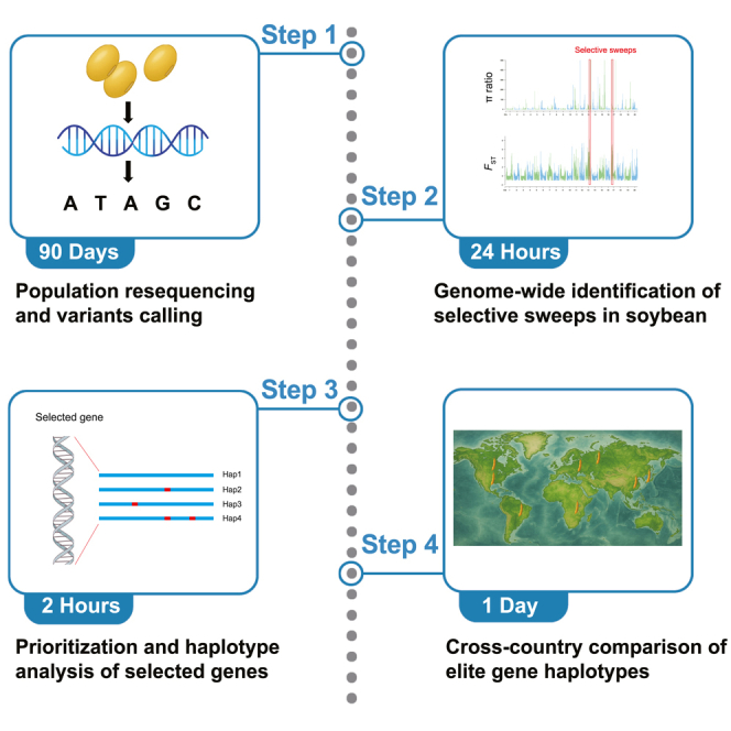 Figure 1
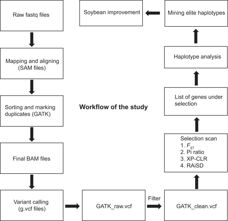 Figure 2
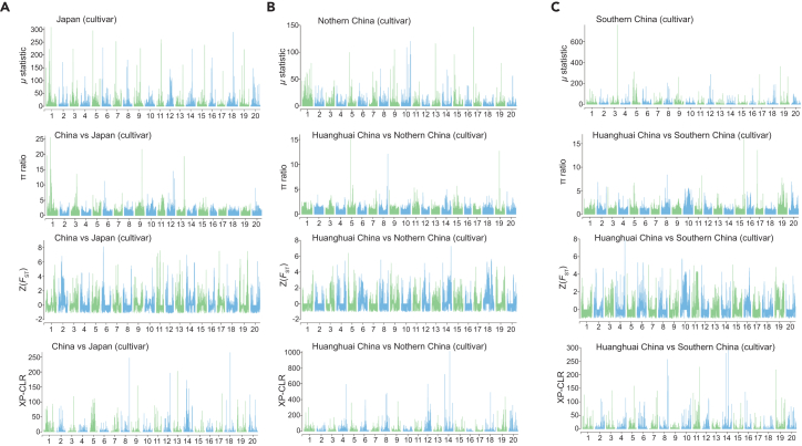 Figure 3
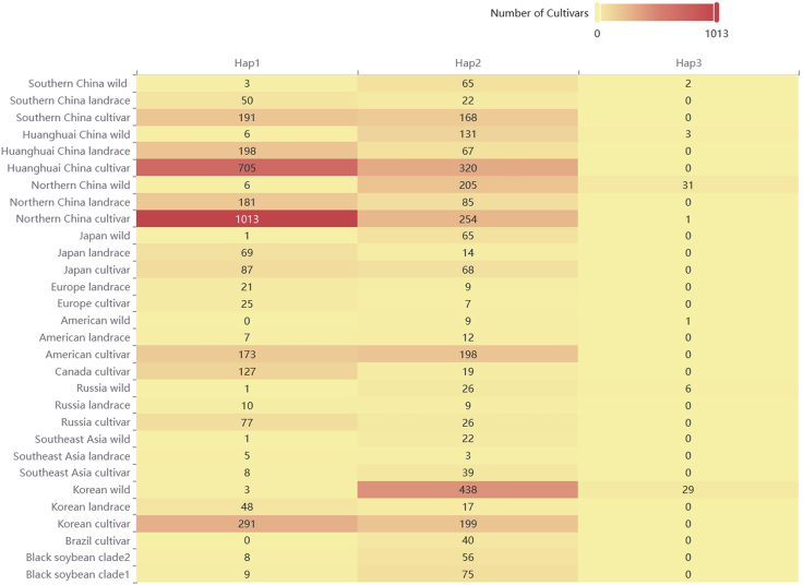 Figure 4
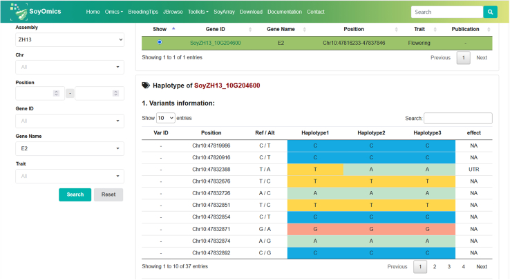 Figure 5
Peer Reviews
No public reviews on file for this paper yet. If you reviewed it on a platform where reviews are public (OpenReview, ICLR, NeurIPS, ICML), you can paste yours below so the community can read it here.
Videos
No videos yet. Explain this paper in a talk, walkthrough, or lecture? Add one.
Taxonomy
TopicsSoybean genetics and cultivation · Phytoestrogen effects and research · Genetic diversity and population structure
Before you begin
This protocol leverages publicly available soybean resequencing data collected from multiple studies deposited in NCBI and the National Genomics Data Center of China. To ensure reliable detection of selected genes and accurate haplotype analysis, raw sequencing data must meet strict quality standards (e.g., high-quality genome resequencing data with sufficient sequencing depth, uniform coverage, and minimal missing sites to ensure completeness and accuracy). Detailed sample information, including accession identifiers, geographic origin, and population metadata, should be verified and curated prior to downstream analysis.
Preparation 1: Data access and quality control
Timing: Variable (affected by dataset size, internet speed, and computational resources)
- 1.Obtain raw resequencing data:
- a.Collect published data or newly generated soybean whole-genome DNA sequencing data in FASTQ format from the sequencing facility.
- b.Confirm that metadata (sample identifiers, population origin, and experimental design) are provided together with the raw data.
- c.Ensure that sequencing was performed with sufficient coverage (average depth ≥ 5×) for downstream variant calling and haplotype analysis.
CRITICAL: Verify that the sequencing facility provides complete documentation on library preparation, sequencing platform, and read length, as inconsistencies can affect data comparability.
- 2.Verify data integrity:
- a.Check file completeness and integrity using checksum files (e.g., MD5).
- b.Ensure that all samples are accounted for and properly named according to the metadata sheet.
- c.Inspect a subset of FASTQ files with tools such as FastQC to confirm overall quality (base quality distribution, adapter contamination, and read length).
CRITICAL: Exclude or request replacement for samples that fail integrity or quality checks before proceeding to downstream processing.
Preparation 2: Setting up the software environment
Timing: 1 h
- 3.Install all required software in a Linux environment, preferably using Conda. We applied multiple complementary population genetic metrics to ensure robust detection of selective signals:
- a.Weir and Cockerham’s FST, calculated using VCFtools, to measure pairwise population differentiation.
- b.π ratio, computed with VCFtools, to identify regions exhibiting reduced nucleotide diversity indicative of selective sweeps.
- c.XP-CLR (Cross-Population Composite Likelihood Ratio) analysis, performed using the XP-CLR software, to detect cross-population selection based on allele frequency differentiation.
- d.RAiSD (Raised Accuracy in Sweep Detection), used to capture signatures of selective sweeps by modeling local distortions in the site frequency spectrum and linkage disequilibrium.
environment.yml
name: python_env
channels:
- bioconda
- conda-forge
- defaults
dependencies:
- python=3.7
- bwa=0.7.18
- trimmomatic=0.39
- samtools=1.20
- gatk4=4.2
- vcftools=0.1.16
- xpclr
- beagle=5.4
# Utilities
- wget
- unzip
# Note: RAiSD is NOT available through conda.
# mkdir RAiSD && cd RAiSD
# wget https://github.com/alachins/raisd/archive/master.zip
# unzip master.zip
# cd raisd-master
# chmod +x install-RAiSD.sh
# ./install-RAiSD.sh
CRITICAL: Ensure that the following software versions are compatible to prevent conflicts during analysis. When version mismatches occur or dependencies cannot be resolved, install individual tools in separate Conda environments.
Innovation
This protocol introduces several advancements over existing approaches for identifying selected genes in soybean.
- 1.Integration of multiple algorithms.2^,^3^,^4^,^5 This workflow combines results from several established algorithms rather than relying on a single detection method, which reduces bias and improves the reliability of identifying genomic regions under selection.
- 2.Customized gene extraction. Tailored scripts are used to automatically extract genes located within candidate intervals, providing a direct and efficient link between statistical signals and biological targets.
- 3.Haplotype-level utilization analysis. By leveraging a high-density variation map and detailed sample metadata, the protocol characterizes haplotype structures for each selected gene and evaluates their distribution across populations from different geographic regions.
Together, these innovations establish a reproducible and versatile workflow that connects selection signals with functional haplotype diversity, offering insights into soybean domestication and breeding.6
Key resources table
REAGENT or RESOURCESOURCEIDENTIFIERDeposited dataSoybean DNA sequencing dataLu et al.7NGDC BioProject: PRJCA001691Soybean DNA sequencing dataLiu et al.8NGDC BioProject: PRJCA002030Soybean DNA sequencing dataYang et al.9NGDC BioProject: PRJCA002554Soybean DNA sequencing dataKajiya-Kanegae et al.10BioProject: PRJDB7250Soybean DNA sequencing dataKajiya-Kanegae et al.10BioProject: PRJDB7386Soybean DNA sequencing dataKajiya-Kanegae et al.10BioProject: PRJDB7786Soybean DNA sequencing dataN/ABioProject: PRJEB1942Soybean DNA sequencing dataN/ABioProject: PRJEB31453Soybean DNA sequencing dataN/ABioProject: PRJNA175477Soybean DNA sequencing dataN/ABioProject: PRJNA227063Soybean DNA sequencing dataN/ABioProject: PRJNA243933Soybean DNA sequencing dataN/ABioProject: PRJNA248222Soybean DNA sequencing dataFang et al.11BioProject: PRJNA257011Soybean DNA sequencing dataN/ABioProject: PRJNA274295Soybean DNA sequencing dataTorkamaneh and Belzile12BioProject: PRJNA287266Soybean DNA sequencing dataValliyodan et al.13BioProject: PRJNA289660Soybean DNA sequencing dataN/ABioProject: PRJNA291452Soybean DNA sequencing dataN/ABioProject: PRJNA294227Soybean DNA sequencing dataN/ABioProject: PRJNA295763Soybean DNA sequencing dataN/ABioProject: PRJNA356132Soybean DNA sequencing dataN/ABioProject: PRJNA383915Soybean DNA sequencing dataN/ABioProject: PRJNA384190Soybean DNA sequencing dataFang et al.11BioProject: PRJNA394629Soybean DNA sequencing dataN/ABioProject: PRJNA449253Soybean DNA sequencing dataN/ABioProject: PRJNA484078Soybean DNA sequencing dataN/ABioProject: PRJNA552939Soybean DNA sequencing dataKim et al.14BioProject: PRJNA555366Soybean DNA sequencing dataN/ABioProject: PRJNA597660Soybean DNA sequencing dataN/ABioProject: PRJNA639876Soybean DNA sequencing dataN/ABioProject: PRJNA681974Soybean DNA sequencing dataN/ABioProject: PRJNA743225Software and algorithmsBWA 0.7.18-r1243-dirtyLi and Durbin15https://sourceforge.net/projects/bio-bwa/Trimmomatic 0.39usadellabhttps://github.com/usadellab/TrimmomaticSAMtools 1.20Li et al.16https://sourceforge.net/projects/samtools/GATK v.4.2McKenna et al.17https://github.com/broadinstitute/gatk/VCFtools 0.1.16Danecek et al.18https://vcftools.github.io/man_latest.htmlRAiSD v.2.9Alachiotis and Pavlidis5https://github.com/alachins/raisdBEAGLE v.5.4Pook et al.19https://faculty.washington.edu/browning/beagle/XpclrVatsiou et al.2https://github.com/hardingnj/xpclrOtherSoybean ZH13.v2 reference genomeThis paperhttps://ngdc.cncb.ac.cn/soyomics/static/data/download/genome/ZH13.v2.fasta.gzThe code and scripts employed for the analyses in this studyThis paperhttps://github.com/sibs-zz/ScricptsForSoybeanOnline platform for querying haplotype analysis of selected genesThis paperhttps://ngdc.cncb.ac.cn/soyomics/breedingtips
Step-by-step method details
Alignment and variant calling
Timing: 72 h
This section focuses on processing raw sequencing reads, aligning them to the reference genome, and generating variant-ready BAM/VCF files for downstream selection and haplotype analysis. A workflow diagram (Figure 1) is also provided to illustrate the input/output relationships across all major steps.
- 1.Read preprocessing with Trimmomatic.
- a.Use Trimmomatic to remove adapter sequences and low-quality bases.
- b.Parameters: ILLUMINACLIP:TruSeq3-PE.fa:2:30:10 for adapter clipping, with additional trimming to ensure high-quality paired-end reads.
- 2.Read alignment with BWA-MEM. Figure 1. Overview of the data processing pipelineThe workflow summarizes key processes including quality control, trimming, alignment to the reference genome, post-alignment processing, variant calling and downstream analysis.
Align cleaned paired-end reads to the soybean reference genome.# Run BWA-MEM alignmentbwa mem \ -t 4 \ -M \ -R "@RG\tID:sampleID\tPL:Illumina\tSM:sample" \ reference.fa \ sample_1_val_1.fq.gz \ sample_2_val_2.fq.gz \ > sample.sam
- 3.Convert SAM to BAM with Samtools.
Convert SAM file to BAM format and filter out secondary alignmentssamtools view \ -F 0x100 \ -Sb \ sample.sam \ > sample.bam
- 4.Sorting BAM with GATK SortSam.
Sort BAM file by genomic coordinates using GATK SortSamgatk SortSam \ --INPUT sample.bam \ --OUTPUT sample_sort.bam --SORT_ORDER coordinate
- 5.Duplicate marking with GATK MarkDuplicates.
Mark duplicate reads using GATK MarkDuplicatesgatk MarkDuplicates \ --INPUT sample_sort.bam \ --OUTPUT sample_sort_MDup.bam \ --METRICS_FILE sample_sort_MDup_metrics.txt \ --VALIDATION_STRINGENCY SILENT \ --OPTICAL_DUPLICATE_PIXEL_DISTANCE 100 \ --ASSUME_SORT_ORDER coordinate \ --CREATE_INDEX trueNote: Parameter OPTICAL_DUPLICATE_PIXEL_DISTANCE should be set to 2500 for patterned flowcell-based sequencers.
- 6.Variant calling with GATK HaplotypeCaller.
Call genomic variants and generate GVCF file using GATK HaplotypeCallergatk HaplotypeCaller \ -R reference.fa \ -I sample_sort_MDup.bam \ -O sample.g.vcf \ -ERC GVCF
Joint genotyping and variant filtering
Timing: Variable (weeks to months depending on sample size)
- 7.Combine GVCFs.
Merge per-sample GVCFs into a single dataset.# Combine individual GVCF files into a single cohort GVCF for joint genotypinggatk CombineGVCFs \ -R reference.fa \ -V sample1.g.vcf \ -V sample2.g.vcf \ ... \ -O cohort.g.vcf
- 8.Joint genotyping with GATK GenotypeGVCFs.
Perform cohort-level genotyping to produce a unified VCF file.# Perform joint genotyping on the combined cohort GVCF to generate a final VCF filegatk GenotypeGVCFs \ -R reference.fa \ -V cohort.g.vcf \ -O cohort.vcf
- 9.Variant filtering.
Apply quality-based filtering to remove low-confidence variants.# Apply quality-based filters to raw variants using GATK VariantFiltrationgatk VariantFiltration \ -R reference.fa \ -V cohort.vcf \ --filter-expression "QD < 2.0 || FS > 60.0 || MQ < 40.0" \ --filter-name "basic_snp_filter" \ -O cohort_filtered.vcfNote: Joint genotyping and variant filtering are highly resource-intensive when dealing with thousands of high-depth resequencing samples. The process may take several weeks to months depending on sample size. It is strongly recommended to use a high-performance computing (HPC) environment with cluster scheduling, parallel execution, and GPU acceleration where available. For large datasets, splitting the genome into intervals and processing them in parallel can dramatically reduce runtime.
FST-based detection of selective sweeps
Timing: 3 h
This section identifies putative selective sweeps by contrasting populations with windowed FST, standardizing scores, and mapping high-signal intervals to genes.
- 10.Inputs and population files.
- a.Prepare a filtered, high-quality cohort VCF (The VCF file used in this step is generated from Step 9. We applied additional quality control using VCFtools, filtering for biallelic single nucleotide polymorphisms (SNPs) with a minor allele frequency (MAF) ≥ 0.05 and missing rate ≤ 0.9).
- b.Create two text files listing sample IDs for each population (one ID per line), e.g., sample1.list and sample2.list. Ensure VCF sample names match the lists exactly.
sample1.list (one sample ID per line)SampleASampleBSampleC# sample2.list (one sample ID per line)SampleDSampleESampleF
- 11.Compute windowed FST with VCFtools.
Calculate population differentiation (Fst) between two groups using VCFtoolsvcftools \ --vcf input.filtered.vcf \ --weir-fst-pop sample1.list \ --weir-fst-pop sample2.list \ --out output_prefix \ --fst-window-size 100000 \ --fst-window-step 10000# Example of output file: output_prefix.windowed.weir.fst# CHROM BIN_START BIN_END N_VARIANTS WEIGHTED_FST MEAN_FST# 1 1 100000 185 0.0245 0.0261# 1 10001 110000 197 0.0283 0.0290# 1 20001 120000 203 0.0327 0.0341
- 12.Clean and extract window statistics.
Extract chromosome, window start, window end, and Fst value columns from the VCFtools outputtail -n +2 output_prefix.windowed.weir.fst \ | cut -f1,2,3,5 \ > output_prefix.fst.window# Example of output file: output_prefix.fst.window# 1 1 100000 0.0245# 1 10001 110000 0.0283# 1 20001 120000 0.0327
- 13.Z-score standardization across windows.
Compute z-scores for windowed Fst values (add a 5th column 'z_score')python zscore.py \ output_prefix.fst.window \ output_prefix.fst.window.zscore# zscore.pyimport sysimport pandas as pdfrom scipy.stats import zscoredef calculate_zscore(input_file, output_file): # Load the data from the file data = pd.read_csv(input_file, sep=" ", header=None) # Ensure the data has at least four columns if data.shape[1] < 4: raise ValueError("Input file must contain at least four columns.") # Calculate z-score for the fourth column data['z_score'] = zscore(data.iloc[:, 3]) # Save the data with the z-score to the output file data.to_csv(output_file, sep=' ', index=False, header=False)if name == "main": if len(sys.argv) != 3: print("Usage: python script.py <input_file> <output_file>") else: input_file = sys.argv[1] output_file = sys.argv[2] calculate_zscore(input_file, output_file)
- 14.Select outlier windows (e.g., Z ≥ 1.96).
Extract candidate regions with significant selection signals (Z ≥ 1.96)awk '$5 >= 1.96' output_prefix.fst.window.zscore | cut -d' ' -f1-3 \ > output_prefix.fst.window.zscore.pos# Example of output file: output_prefix.fst.window.zscore.pos# 1 60001 160000# 1 70001 170000# 1 80001 180000
- 15.Normalize chromosome labels to match the GFF.
Normalize chromosome names: add leading zero if <10 (e.g., Chr01, Chr02, ...)awk '1<10 {printf("Chr0%s %s %s\n",1,3)} 1>=10 {printf("Chr%s %s %s\n",1,3)}' \ output_prefix.fst.window.zscore.pos \ > output_prefix.fst.window.zscore.pos.norm# Example of output file: output_prefix.fst.window.zscore.pos.norm# Chr01 60001 160000# Chr01 70001 170000# Chr01 80001 180000
- 16.Map outlier intervals to genes (GFF overlap).
Extract overlapping genes from GFF for the candidate windowspython GetGeneFromGFF.py reference.gff \ output_prefix.fst.window.zscore.pos.norm \ output_prefix.fst.window.zscore.pos.genes# GetGeneFromGFF.pyimport pandas as pdimport sysdef read_gff(gff_path): columns = ['seqname', 'source', 'feature', 'start', 'end', 'score', 'strand', 'frame', 'attributes'] gff_df = pd.read_csv(gff_path, sep='\t', comment='#', names=columns) genes_df = gff_df[gff_df['feature'] == 'gene'] return genes_dfdef read_bed(bed_path): columns = ['chrom', 'start', 'end', 'name'] bed_df = pd.read_csv(bed_path, sep=r'\s+', names=columns) return bed_dfdef extract_genes_from_regions(gff_df, bed_df): extracted_genes = [] for index, row in bed_df.iterrows(): region_genes = gff_df[(gff_df['seqname'] == row['chrom']) & (gff_df['start'] <= row['end']) & (gff_df['end'] >= row['start'])] extracted_genes.append(region_genes) return pd.concat(extracted_genes) if extracted_genes else pd.DataFrame()def main(gff_path, bed_path, output_path): gff_df = read_gff(gff_path) bed_df = read_bed(bed_path) genes = extract_genes_from_regions(gff_df, bed_df) genes.to_csv(output_path, index=False, sep='\t')if name == "main": gff_path, bed_path, output_path = sys.argv[1:4] main(gff_path, bed_path, output_path)
- 17.Extract unique gene IDs (candidate selected genes).
Extract unique gene IDs from GFF annotation results (remove duplicates and clean attributes)awk -F '\t' '{print $9}' output_prefix.fst.window.zscore.pos.genes \ | grep -v attr \ | sed 's/ID=//g' \ | sed 's/;//g' \ | sort -u \ > output_prefix.fst.window.zscore.pos.genes.clean# Example of raw gene list with duplicates (output_prefix.fst.window.zscore.pos.genes)# SoyZH13_01G003210# SoyZH13_02G045870# SoyZH13_02G045870# SoyZH13_03G100155# SoyZH13_04G009900# SoyZH13_05G201234# SoyZH13_05G201234# Example of cleaned, deduplicated output file (output_prefix.fst.window.zscore.pos.genes.clean)# SoyZH13_01G003210# SoyZH13_02G045870# SoyZH13_03G100155# SoyZH13_04G009900# SoyZH13_05G201234Note: Ensure the same reference build is used for both the VCF and the GFF annotation file. Choice of window size and step (e.g., 100 kb/10 kb) will affect resolution; justify and report parameter choices.
Nucleotide diversity (π) analysis and π-ratio-based sweep detection
Timing: 3 h
This section computes windowed nucleotide diversity (π) for two populations, derives the π ratio (popA/popB) on common windows, standardizes scores, and maps outlier intervals to genes.
- 18.Inputs and population files.
- a.Filtered cohort VCF: input.filtered.vcf (biallelic SNPs; recommended MAF/missingness filters).
- b.Two population lists with sample IDs: popA.list, popB.list (one ID per line).
- c.Gene annotation: reference.gff.
- d.Utility scripts: zscore.py for Z-score standardization; GetGeneFromGFF.py for interval to gene mapping.
- 19.Prepare per-population π jobs (windowed).
Create a shell script to run windowed π for each population list (100 kb windows; 100 kb steps shown as example).# Generate per-population π calculation commands and save them into run_pi.shls ∗.list | while read plistdo echo "nohup vcftools \ --vcf input.filtered.vcf \ --keep {plist%.list} &" done > run_pi.sh && sh run_pi.sh
- 20.Extract window keys and intersect common windows.
Extract common genomic windows shared between two populations (popA and popB)grep -v BIN popA.windowed.pi \ | awk -F ' ' '1 && 2 && 3 {print 1""3}' \ | sort \ > A.keysgrep -v BIN popB.windowed.pi \ | awk -F ' ' '1 && 2 && 3 {print 1""3}' \ | sort \ > B.keyscomm -12 A.keys B.keys > common.keys
- 21.Prefix π tables with window keys for joining.
Tag each row with a composite window keyawk '{print 2""0}' popA.windowed.pi > A.tagawk '{print 2""0}' popB.windowed.pi > B.tag# Pull rows for common windowswhile read k; do grep -w "k" B.tag; done < common.keys > B.common
- 22.Join tables, compute π ratio, and tidy. Note: In VCFtools windowed.pi, π is typically in column 4 (PI). Adjust field indices if your format differs.# Compute π ratio per common windowpaste A.common B.common \ | awk '{print 3, 6, 6/12}' \ > popA_vs_popB.piratio # CHR START END PI_A PI_B PIratio# Sort by chromosome and start, then keep CHR START END PIratiogrep -v BIN popA_vs_popB.piratio \ | sort -k1,1n -k2,2n \ | awk '{print 1, 3, $6}' \ > popA_vs_popB.piratio.in
- 23.Z-score standardization and outlier selection.
Calculate Z-scores for π ratio valuespython zscore.py \ popA_vs_popB.piratio.in \ popA_vs_popB.piratio.in.zscore# Extract genomic windows with significant Z-scores (Z ≥ 1.96)awk '5 >= 1.96 {print 1, 3}' \ popA_vs_popB.piratio.in.zscore \ > popA_vs_popB.piratio.in.zscore.pos
- 24.Normalize chromosome labels to match the GFF (if needed).
Normalize chromosome naming (add leading zeros, e.g., Chr01-Chr09)awk '1 < 10 {printf("Chr0%s %s %s\n", 1, 3)} \ 1 >= 10 {printf("Chr%s %s %s\n", 1, 3)}' \ popA_vs_popB.piratio.in.zscore.pos \ > popA_vs_popB.piratio.in.zscore.pos.norm
- 25.Map outlier intervals to genes.
Extract overlapping genes from GFF for candidate selective regionspython GetGeneFromGFF.py \ reference.gff \ popA_vs_popB.piratio.in.zscore.pos.norm \ popA_vs_popB.piratio.in.zscore.pos.genes# Extract and clean unique gene IDs from the GFF-derived tableawk '{print $9}' popA_vs_popB.piratio.in.zscore.pos.genes | grep -v attr \ | sed 's/ID=//g' \ | sed 's/;//g' \ | sort -u \ > popA_vs_popB.piratio.in.zscore.pos.genes.cleanNote: Use identical window size and step for both populations; π ratios are meaningful only on common windows. Ensure consistent reference build and contig naming across VCF and GFF; normalize labels before overlap.
RAiSD-based detection of selective sweeps
Timing: 24 h
This section runs RAiSD to compute the composite sweep statistic (μ), aggregates per-chromosome reports, standardizes scores, and maps high-signal intervals to genes.
- 26.Run RAiSD on the cohort.
Detect genomic regions under selection using RAiSD ./raisd-master/bin/release/RAiSD \ -n popA \ -I input.filtered.vcf \ -R \ -A 0.95 \ -S popA.list \ -f
Output: per-chromosome reports named like RAiSD_Report.popA.1, RAiSD_Report.popA.2, …
- 27.Aggregate per-chromosome reports into one table.
Merge RAiSD results from all chromosomes into a single summary file: > popA.RAiSD.allfor f in RAiSD_Report.popA.∗do chr=f" | awk -F. 'NF {print NF}') awk '{printf "%.3f %.3f %.3f\n", 2, 7}' "chr" '{print c, $0}' \ >> popA.RAiSD.alldone
- 28.Z-score standardization across genome-wide windows.
Normalize RAiSD statistics using Z-score transformationpython zscore.py \ popA.RAiSD.all \ popA.RAiSD.all.zscore
- 29.Select outlier windows (e.g., Z ≥ 1.96).
Extract genomic regions showing significant selection signals (Z ≥ 1.96)awk '5 >= 1.96 {print 1, 3}' \ popA.RAiSD.all.zscore \ > popA.RAiSD.outliers.pos
Adjust the cutoff (e.g., top 1%/5%) according to study design.
- 30.Normalize chromosome labels to match the GFF (if needed).
Normalize chromosome naming format for downstream gene mappingawk '1 < 10 {printf "Chr0%s %s %s\n", 1, 3} \ 1 >= 10 {printf "Chr%s %s %s\n", 1, 3}' \ popA.RAiSD.outliers.pos \ > popA.RAiSD.outliers.norm
- 31.Map outlier intervals to genes and extract unique IDs.
Extract candidate genes overlapping with significant selection regionspython GetGeneFromGFF.py \ reference.gff \ popA.RAiSD.outliers.norm \ popA.RAiSD.outliers.genes# Clean and deduplicate extracted gene list (SoyZH13 gene IDs)awk '{print $9}' popA.RAiSD.outliers.genes \ | grep -v attr \ | sed 's/ID=//g' \ | sed 's/;//g' \ | sort -u \ > popA.RAiSD.outliers.genes.cleanNote: Use the same reference build and contig naming across VCF, RAiSD outputs, and reference.gff. For large cohorts/VCFs, parallelize by chromosome and run on HPC to mitigate I/O and CPU bottlenecks; keep intermediate files compressed and document software versions for reproducibility.
XP-CLR-based detection of selective sweeps
Timing: 24 h
This section computes XP-CLR between two populations across all chromosomes, aggregates scores, standardizes them, and maps high-signal intervals to genes.
- 32.Inputs and population files.
- a.Filtered cohort VCF: input.filtered.vcf (biallelic SNPs; uniform MAF/missingness filters).
- b.Two population lists with sample IDs: popA.list, popB.list (one ID per line).
- c.Gene annotation: reference.gff.
- d.Utility scripts: zscore.py for standardization; GetGeneFromGFF.py for interval to gene mapping.
- 33.Run XP-CLR per chromosome.
Example parameters shown: LD cutoff 0.95, max 1000 SNPs per window, 100 kb window/step. Adjust to your design.# Bash loop over chromosome IDs 1..20 (edit range for your genome)for chr in {chr} \ -Sa popA.list \ -Sb popB.list \ --input input.filtered.vcf \ --chr ${chr} \ --ld 0.95 \ --maxsnps 1000 \ --size 100000 \ --step 100000done
Output: one file per chromosome (e.g., popA_vs_popB_chr1, popA_vs_popB_chr2, …).
- 34.Concatenate chromosome outputs.
Keep header from the first file, append non-header lines from the resthead -1 popA_vs_popB_chr1 > popA_vs_popB_allchrfor chr in {chr} >> popA_vs_popB_allchrdone
- 35.Extract genomic coordinates and XP-CLR score. Note: Typical XP-CLR outputs contain chromosome, window start/end, and the XP-CLR statistic; adjust column indices if your format differs.# Extract chromosome position and XP-CLR score columns, remove headers and malformed linesawk '{print 3, 12}' popA_vs_popB_allchr \ | grep -v xpclr \ | awk 'NF == 4' \ > popA_vs_popB_allchr.score
- 36.Z-score standardization and outlier selection.
Normalize XP-CLR scores using Z-score transformationpython zscore.py \ popA_vs_popB_allchr.score \ popA_vs_popB_allchr.score.z# Identify genomic windows with significant XP-CLR signals (Z ≥ 1.96)awk '5 >= 1.96 {print 1, 3}' \ popA_vs_popB_allchr.score.z \ > popA_vs_popB_allchr.outlier.pos
- 37.Normalize chromosome labels to match the GFF (if needed).
Normalize chromosome naming format for consistency with reference genome (e.g., Chr01-Chr20)awk '1 < 10 {printf "Chr0%s %s %s\n", 1, 3} \ 1 >= 10 {printf "Chr%s %s %s\n", 1, 3}' \ popA_vs_popB_allchr.outlier.pos \ > popA_vs_popB_allchr.outlier.pos.norm
- 38.Map outlier windows to genes and deduplicate IDs.
Extract candidate genes overlapping with XP-CLR outlier regionspython GetGeneFromGFF.py \ reference.gff \ popA_vs_popB_allchr.outlier.pos.norm \ popA_vs_popB_allchr.outlier.genes# Clean and deduplicate extracted gene list (SoyZH13 gene IDs)awk '{print $9}' popA_vs_popB_allchr.outlier.genes \ | grep -v attr \ | sed 's/ID=//g' \ | sed 's/;//g' \ | sort -u \ > popA_vs_popB_allchr.outlier.genes.cleanNote: Use the same reference build and consistent contig names across VCF, XP-CLR outputs, and reference.gff; normalize labels before overlap. Window size, step, LD cutoff, and --maxsnps strongly affect sensitivity and runtime; report chosen values and run sensitivity checks.
Consensus integration of candidate genes across methods
Timing: 5 min
This section merges candidate gene lists from multiple detection approaches (e.g., FST, π-ratio, XP-CLR, RAiSD). It supports flexible thresholds such as “identified by ≥1 method”, “≥2 methods”, or “≥3 methods”.
- 39.Inputs (one gene ID per line):
Make sure each file contains a single column of standardized gene IDs (no headers). If your IDs include attributes (e.g., ID=...;), clean them first as shown in earlier steps.
- 40.Streamlined code for merging gene lists.# Set threshold K (e.g., 1, 2, 3...)K=2# Merge all gene lists and compute support countscat ∗.outlier.genes.clean \ | sort \ | uniq -c \ > gene.counts.tmp# Genes supported by ≥K methodsawk -v k=K '{if (1 >= k) print 2}' gene.counts.tmp \ > consensus.k{K}.genes# Genes supported by exactly K methods (optional)awk -v k=K '{if (1 == k) print 2}' gene.counts.tmp \ > consensus.eqk{K}.genesNote: This code concatenates all input lists, counts the number of methods supporting each gene, and outputs two files:
- a.consensus.kK.genes: genes detected by at least K methods.
- b.consensus.eqkK.genes: genes detected by exactly K methods.Ensure all lists use the same gene ID namespace (e.g., ZH13). If needed, map aliases to a canonical ID before merging. Record software versions and thresholds (window sizes, Z cutoffs). Store the exact shell commands in your workflow log or Makefile/Snakemake.
Haplotype extraction and statistics
Timing: 5 min
This section extracts a target genomic interval from cohort VCFs, phases/genotypes (if needed), enumerates unique haplotypes per sample, and summarizes haplotype counts by geographic/population groups.
- 41.Inputs.
- a.Per-chromosome, bgzipped + tabix-indexed VCFs: .../vcf/soybean.∗.Chr∗.vcf.gz.
- b.Target interval: for example Chr2:50394718-50402312.
- c.Sample group lists (one sample ID per line), e.g., regionA.list, regionB.list, …
- d.Gene annotation (optional, for downstream mapping).
- e.haplo.py (the provided pysam script that prints per-sample haplotypes and labels them Haplotype1/2/...).
haplo.pyimport pysamimport sysfrom collections import defaultdictvcf = pysam.VariantFile(vcf_path)haplotypes = defaultdict(lambda: [])valid_positions = set()for record in vcf: if all(record.samples[sample]['GT'] is not None for sample in record.samples): valid_positions.add(record.pos)for record in vcf: if record.pos in valid_positions: for sample in record.samples: gt = record.samples[sample]['GT'] haplotypes[sample].append(gt)haplotypes_str = {sample: str(gt_list) for sample, gt_list in haplotypes.items()}unique_haplotypes = defaultdict(lambda: [])for sample, haplotype in haplotypes_str.items():unique_haplotypes[haplotype].append(sample)filtered_haplotypes = {k: v for k, v in unique_haplotypes.items() if len(v) >= 1}sorted_haplotypes = sorted(filtered_haplotypes.items(), key=lambda x: len(x[1]), reverse=True)for idx, (haplotype, samples) in enumerate(sorted_haplotypes, start=1): print(f"Haplotype{idx}: {haplotype}, Count: {len(samples)}") for sample in samples: print(f" Haplo{idx}: {sample}")vcf.close()
- 42.Extract the interval across all per-chromosome VCFs.
Pull the interval from every per-chromosome VCF and merge, then sort by POSls ../vcf/soybean.∗.Chr∗vcf.gz | while read v; do tabix "$v" Chr2:50394718-50402312done | sort -k2,2n > interval.recordsNote: If you also need a VCF header, capture it once from any matching VCF.zcat ../vcf/soybean.X.Chr2.vcf.gz | grep # > header.vcf
- 43.Assemble a minimal interval VCF: cat header.vcf interval.records > interval.raw.vcf
- 44.Phase/impute (recommended).
If your cohort isn’t fully phased or has sporadic missing genotypes, phase with Beagle on the interval.beagle gt=interval.vcf out=interval_beagle# Output: interval_beagle.vcf.gz
- 45.Call haplotypes per sample (across valid sites).python haplo.py interval_beagle.vcf.gz > interval.haploThe script.
- a.Loads all biallelic sites with complete genotypes across samples (“valid positions”).
- b.Builds a per-sample haplotype string over the valid sites.
- c.Prints unique haplotypes as Haplotype1, Haplotype2, … with member sample IDs.Example output (abridged).Haplotype1: [...] , Count: 4223 Haplo1: SAMPLE_A01 Haplo1: SAMPLE_A02 ...Haplotype2: [...] , Count: 1786 Haplo2: SAMPLE_B03 ...
- 46.Count haplotypes by region/population.
For each region list (e.g., regionA.list), count how many listed samples fall into each haplotype.# Count members of Haplotype1..Haplotype5 in regionAfor k in 1 2 3 4 5; do cat regionA.list \ | while read sid; do grep -w "{k}" \ | wc -ldoneNote: Phasing & missingness: Haplotype inference is sensitive to missing calls and phasing. Use Beagle (or comparable) and require consistent sample sets per locus. Ensure sample IDs and their case match exactly across VCF and region lists.
Expected outcomes
This protocol yields a cohort-level, quality-controlled VCF suitable for selection scans, plus per-method genome-wide statistics and curated gene sets for downstream interpretation. From the four scan approaches (FST, π-ratio, XP-CLR, RAiSD), researchers can expect chromosome-wide score tables (one row per window) that are Z-standardized within method, lists of outlier windows at predefined cutoffs, and interval-to-gene mappings that produce method-specific candidate gene lists. Consolidation across methods generates union and consensus gene sets (e.g., identified by ≥1, ≥2, or ≥3 methods).
Figures should display genome-wide score tracks for all four methods. In a between-population contrast (e.g., China vs Japan, Figure 2A), expect discrete peaks where multiple methods co-localize, indicating putative selective sweeps; within-China regional contrasts typically reveal region-specific peaks (Figures 2B and 2C).Figure 2. Genome-wide selection scans across soybean cultivars from different geographic regions(A) Comparisons between China cultivars and Japan cultivars.(B) Comparisons between Huanghuai China cultivars and Northern China cultivars.(C) Comparisons between Huanghuai China cultivars and Southern China cultivars. For each region, selection signals were identified using multiple statistics, including μ statistic, π ratio, standardized FST, and XP-CLR. Each panel shows the distribution of selection signals along the 20 soybean chromosomes.
Gene-based haplotypes were constructed from high-confidence SNPs using GATK for variant filtering and Beagle for genotype phasing and imputation. Haplotype analysis at candidate loci produces, for each interval, the number of unique haplotypes and a membership list of samples per haplotype. Aggregating by region (e.g., geographic groups within China) yields count tables or heatmaps that visualize haplotype utilization across populations (Figure 3) (more examples can be found in https://ngdc.cncb.ac.cn/soyomics/breedingtips). Typical outcomes include one or more predominant haplotypes per locus with minor alternatives; regionally enriched haplotypes are expected at loci flagged by multiple selection scans.Figure 3. Distribution of E2 (SoyZH13_10G204600) haplotypes among wild, landrace, and cultivated soybean groups across different geographical regionsThe heatmap illustrates the number of accessions carrying each E2 haplotype (Hap1-Hap3) in diverse soybean populations, including wild, landrace, and cultivated groups from various countries and regions. The color gradient represents the number of cultivars, with darker red indicating higher frequency of the corresponding haplotype within a population.
Deliverables include: per-method windowed statistics (with Z-scores), outlier window BED-like files, method-specific candidate gene lists, consensus gene sets at user-defined thresholds, and haplotype count matrices by region. Together, these outputs support narrative results (genome-wide peaks, convergent signals, and region-biased haplotypes) and figure panels illustrating whole-genome statistics for user-specified comparisons.
Overall, this protocol enables the systematic identification of genomic regions and candidate genes under selection by integrating multiple population genetic statistics. By combining these complementary approaches, researchers can pinpoint loci that have undergone selection during domestication or adaptation to diverse environments. The subsequent haplotype analysis allows the characterization of advantageous haplotypes associated with desirable agronomic traits such as yield, flowering time, and stress tolerance. These insights can facilitate the discovery of elite alleles and haplotypes (Figure 4) that contribute to environmental adaptation and yield improvement, providing a foundation for molecular breeding and genetic improvement of soybean.Figure 4. Screenshot of the online soybean haplotype query platform (SoyOmics) showing haplotype structure of the E2 geneThis figure illustrates the web interface developed for querying gene haplotypes in soybean populations. The example shown is for the E2 gene, displaying three major haplotypes and their corresponding SNP variant positions across the gene region. Each column represents a haplotype, while colored cells indicate the allelic states (Ref/Alt) of the SNPs defining each haplotype.
Limitations
This protocol relies on heterogeneous resequencing datasets aggregated from multiple sources; differences in library preparation, sequencing platform, read length, and DNA quality can introduce batch effects that are not fully removed by standard QC and normalization. Uneven or sub-threshold coverage (<∼5×), high missingness, or inaccurate metadata (e.g., mislabeled geographic origin) reduce power and may produce spurious between-population contrasts. Resequencing data newly generated from the same batch of materials through the standardized pipeline of the same sequencing company ensure improved reliability and performance of this analytical workflow.
Reference-related issues—including misassemblies, repetitive/pericentromeric regions with low mappability, and annotation/version mismatches—can distort window statistics and gene mapping, particularly when contig names or builds are inconsistent across VCF and GFF files. Additionally, differences in reference genome assembly quality and annotation versions can result in inconsistent variant detection and may affect the interpretation of selective sweep signals and haplotype structure.
Selection-scan statistics have method-specific sensitivities and assumptions; demographic history (bottlenecks, structure, admixture/introgression) can mimic sweep-like signals, while strong LD or low recombination can inflate scores independent of recent selection. Window-based analyses are sensitive to parameter choices (window size, step, LD cutoff) and Z-score thresholding. Cross-method consensus increases robustness but may miss true positives detectable by only one approach, and it does not by itself resolve demographic confounding without explicit modeling or permutation-based calibration.
Haplotype inference depends on accurate genotypes and phasing. When phasing is imperfect or missingness is nonrandom, inferred haplotypes and their regional counts can be biased. The illustrative haplotype script retains only sites genotyped in all samples; in large cohorts this may discard informative variants and skew haplotype definitions toward common sites. Structural variants, copy-number variation, and presence/absence polymorphisms are largely invisible to SNP-based scans and may underlie genuine adaptation that this workflow will not detect.
Troubleshooting
Problem 1
Adapter contamination or poor base quality leads to low mapping rates. (step 1).
Potential solution
Inspect reads with FastQC; increase trimming stringency (e.g., add SLIDINGWINDOW:4:20, MINLEN=36) and verify ILLUMINACLIP adapters match the library kit.
Users may observe messages such as.
- •“Adapter sequence detected” or excessive adapter content in FastQC reports.
- •“Per base sequence quality: FAIL/WARN” in FastQC.
- •Low alignment rate (<70%) reported by BWA/SAMtools (e.g., “mapped: 65%”).
For each of these problems, we now provide clear solutions, including.
- •Re-running adapter and quality trimming (e.g., with Trimmomatic or fastp).
- •Verifying improvement in per-base quality and adapter removal using FastQC before alignment.
- •Checking for overrepresented sequences or library preparation issues.
Problem 2
SAM to BAM conversion errors or truncated files. (step 3).
Potential solution
- •Check disk space and ulimit; prefer samtools sort pipeline over intermediate SAM.
- •Validate with samtools quickcheck and regenerate if corruption is detected.
Problem 3
Joint genotyping is prohibitively slow or fails. (step 7–8).
Potential solution
- •Use GenomicsDBImport + GenotypeGVCFs instead of CombineGVCFs for large cohorts.
- •Scatter by chromosome/interval; run on HPC with job arrays; keep I/O local (node-local SSD).
- •Confirm consistent sample order and identical reference dictionary across all inputs.
Problem 4
Windowed FST contains NA or unexpected BIN header rows. (step 11).
Potential solution
- •Ensure both population lists match VCF sample IDs; remove empty/typo lines.
- •Apply uniform missingness/MAF filters; drop monomorphic windows.
- •Strip non-data lines before downstream parsing as shown in the workflow.
- •We have added a validation script that automatically checks input and output file formats for consistency and completeness.
#!/usr/bin/env python3
import sys
if len(sys.argv) != 2:
print("Usage: python clean_fst.py <windowed_fst.txt>", file=sys.stderr)
sys.exit(1)
infile = sys.argv[1]
with open(infile) as f:
next(f) # skip header line
for line in f:
if "NA" in line or "NaN" in line or "nan" in line:
continue # skip NA lines
fields = line.strip().split()
if len(fields) < 6:
continue
chrom = fields[0]
start = fields[1]
end = fields[2]
fst = fields[4] # WEIGHTED_FST
print(chrom, start, end, fst, sep="\t")
Problem 5
π-ratio windows do not line up between populations. (step 19).
Potential solution
- •Use identical --window-pi and --window-pi-step for both groups.
- •Intersect common windows (as scripted) before ratio calculation; avoid mixing different filters between groups.
Problem 6
RAiSD outputs missing for some chromosomes or μ distribution looks abnormal. (step 26).
Potential solution
- •Verify chromosome naming matches VCF; run per-chromosome and aggregate with the provided loop.
- •Confirm input MAF filters and SNP density.
Problem 7
XP-CLR reports few or no windows/errors about insufficient SNPs. (step 33).
Potential solution
- •Reduce --maxsnps or increase window size; relax --ld threshold slightly if appropriate.
- •Confirm population lists are non-overlapping and reasonably sized; ensure VCF is biallelic and filtered.
Problem 8
Gene mapping yields zero hits. (All mapping steps using GetGeneFromGFF.py).
Potential solution
- •Normalize contig labels (e.g., Chr02 vs 2) before overlap; ensure GFF and VCF share the same build.
- •Expand windows slightly to accommodate annotation boundaries; verify GFF column conventions.
Problem 9
Haplotype script returns very few sites or no haplotypes. (step 47).
Potential solution
- •The script currently requires all samples to be non-missing at each site; relax this by allowing ≥95% call rate, or phase/impute with Beagle first.
- •Split multiallelics with bcftools norm -m-any and maintain consistent sample sets across loci.
Resource availability
Lead contact
Requests for resources, data, and further information should be addressed to the lead contact, Zhou Zhu ([email protected]).
Technical contact
Technical questions on executing this protocol will be answered by the technical contact, Zhou Zhu ([email protected]).
Materials availability
This study did not generate new reagents.
Data and code availability
The code generated during this study is publicly available on GitHub (https://github.com/sibs-zz/ScricptsForSoybean) and has been archived on Zenodo (DOI: https://doi.org/10.5281/zenodo.17784450).
Acknowledgments
This work was supported by the Yazhouwan National Laboratory Project (2310ZX01), the National Natural Science Foundation of China (grant 32388201), the Xplorer Prize (to Z.T.), and the Taishan Scholars Program (to Z.T.). We thank Professor Guodong Wang (Institute of Genetics and Developmental Biology, Chinese Academy of Sciences) and Professor Dawei Xin (Northeast Agricultural University, Harbin, China) for assistance in this study.
Author contributions
Z.T. supervised the project. Protocol and analysis pipeline were organized and contributed by Z.Z.
Declaration of interests
The authors declare no competing interests.
The reference list from the paper itself. Each links out to its DOI / PubMed record.
- 1Zhu Z.Wang Y.Liu S.Wang S.Li J.Fang C.Liu Y.Yang X.Tian D.Song S.Tian Z.Genomic atlas of 8,105 accessions reveals stepwise domestication, global dissemination, and improvement trajectories in soybean Cell 188202565196535.e 1510.1016/j.cell.2025.09.00741038165 · doi ↗ · pubmed ↗
- 2Vatsiou A.I.Bazin E.Gaggiotti O.E.Detection of selective sweeps in structured populations: a comparison of recent methods Mol. Ecol.2520168910310.1111/mec.1336026314386 · doi ↗ · pubmed ↗
- 3Zhou Z.Jiang Y.Wang Z.Gou Z.Lyu J.Li W.Yu Y.Shu L.Zhao Y.Ma Y.Resequencing 302 wild and cultivated accessions identifies genes related to domestication and improvement in soybean Nat. Biotechnol.33201540841410.1038/nbt.309625643055 · doi ↗ · pubmed ↗
- 4Huang X.Kurata N.Wei X.Wang Z.X.Wang A.Zhao Q.Zhao Y.Liu K.Lu H.Li W.A map of rice genome variation reveals the origin of cultivated rice Nature 490201249750110.1038/nature 1153223034647 PMC 7518720 · doi ↗ · pubmed ↗
- 5Alachiotis N.Pavlidis P.R Ai SD detects positive selection based on multiple signatures of a selective sweep and SNP vectors Commun. Biol.120187910.1038/s 42003-018-0085-830271960 PMC 6123745 · doi ↗ · pubmed ↗
- 6Tian Z.Nepomuceno A.L.Song Q.Stupar R.M.Liu B.Kong F.Ma J.Lee S.H.Jackson S.A.Soybean 2035: A decadal vision for soybean functional genomics and breeding Mol. Plant 18202524527110.1016/j.molp.2025.01.00439772289 · doi ↗ · pubmed ↗
- 7Lu S.Dong L.Fang C.Liu S.Kong L.Cheng Q.Chen L.Su T.Nan H.Zhang D.Stepwise selection on homeologous PRR genes controlling flowering and maturity during soybean domestication Nat. Genet.52202042843610.1038/s 41588-020-0604-732231277 · doi ↗ · pubmed ↗
- 8Liu Y.Du H.Li P.Shen Y.Peng H.Liu S.Zhou G.A.Zhang H.Liu Z.Shi M.Pan-genome of wild and cultivated soybeans Cell 1822020162176.e 1310.1016/j.cell.2020.05.02332553274 · doi ↗ · pubmed ↗