How the Level of Noise Affects Temporal Accuracy of a QRS Detector—Case Study
Wojciech Reklewski, Piotr Augustyniak

TL;DR
This study examines how noise and timing precision affect the accuracy of a QRS detector used in ECG analysis.
Contribution
The paper introduces a new method for evaluating QRS detectors by varying time jitter and noise levels.
Findings
The detector's quality dropped significantly as time jitter tightened from 97.23 ms to 86.12 ms.
Detection quality decreased with increasing noise levels, though some records showed better performance in noisy conditions.
Imprecise local maximum definitions were identified as a cause of detection errors in certain cases.
Abstract
Background: QRS complex detection is a key processing step of automated ECG analysis and determines its overall quality. The purpose of this paper is to study the detection performance of probably the most frequently implemented ready-to-use QRS detector in the presence of noise and with tightened temporal tolerance of detection points. Methods: We applied commonly used detection statistics (Detection Error Rate, Sensitivity, Positive Predictive Value, and F1 score), but re-defined true positive detection based on variable time jitter between detected and reference points. We also applied a controlled level of mixed noise to assess the detector’s performance in true-to-life conditions. Results: We found the following: (1) the detector under test showed a considerable drop in quality when reducing the jitter between 97.23 ms (DER = 8.08%) and 86.12 ms (DER = 67.22%), which means that the…
Genes, proteins, chemicals, diseases, species, mutations and cell lines named across the full text — each resolved to its canonical identifier and authoritative record.
Click any figure to enlarge with its caption.
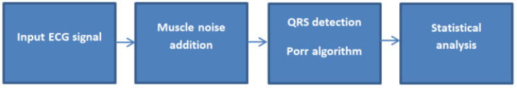 Figure 1
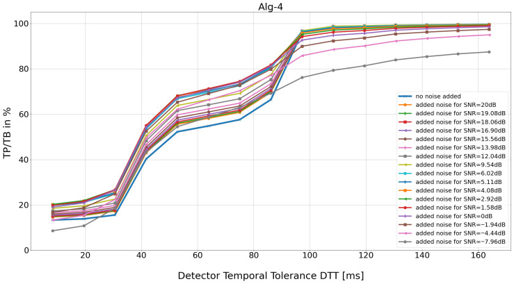 Figure 2
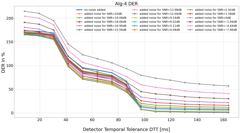 Figure 3
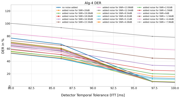 Figure 4
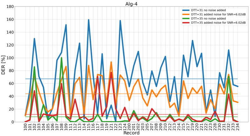 Figure 5
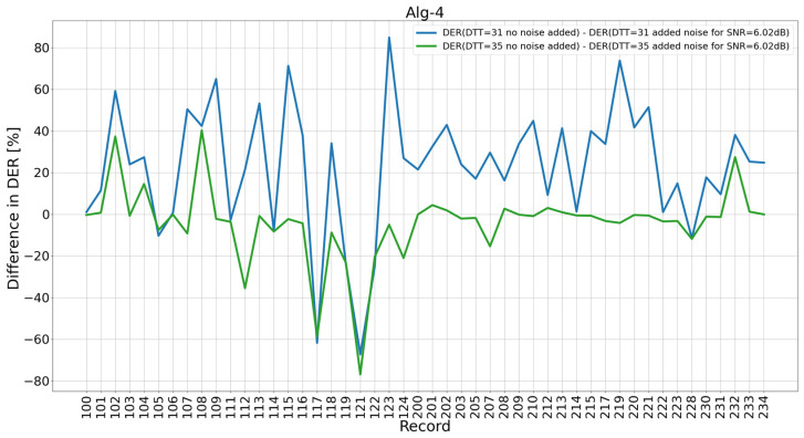 Figure 6
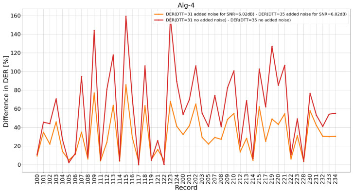 Figure 7
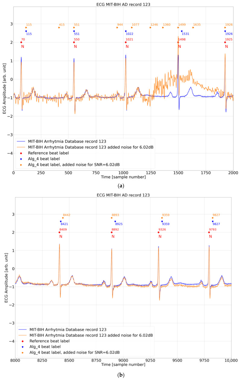 Figure 8
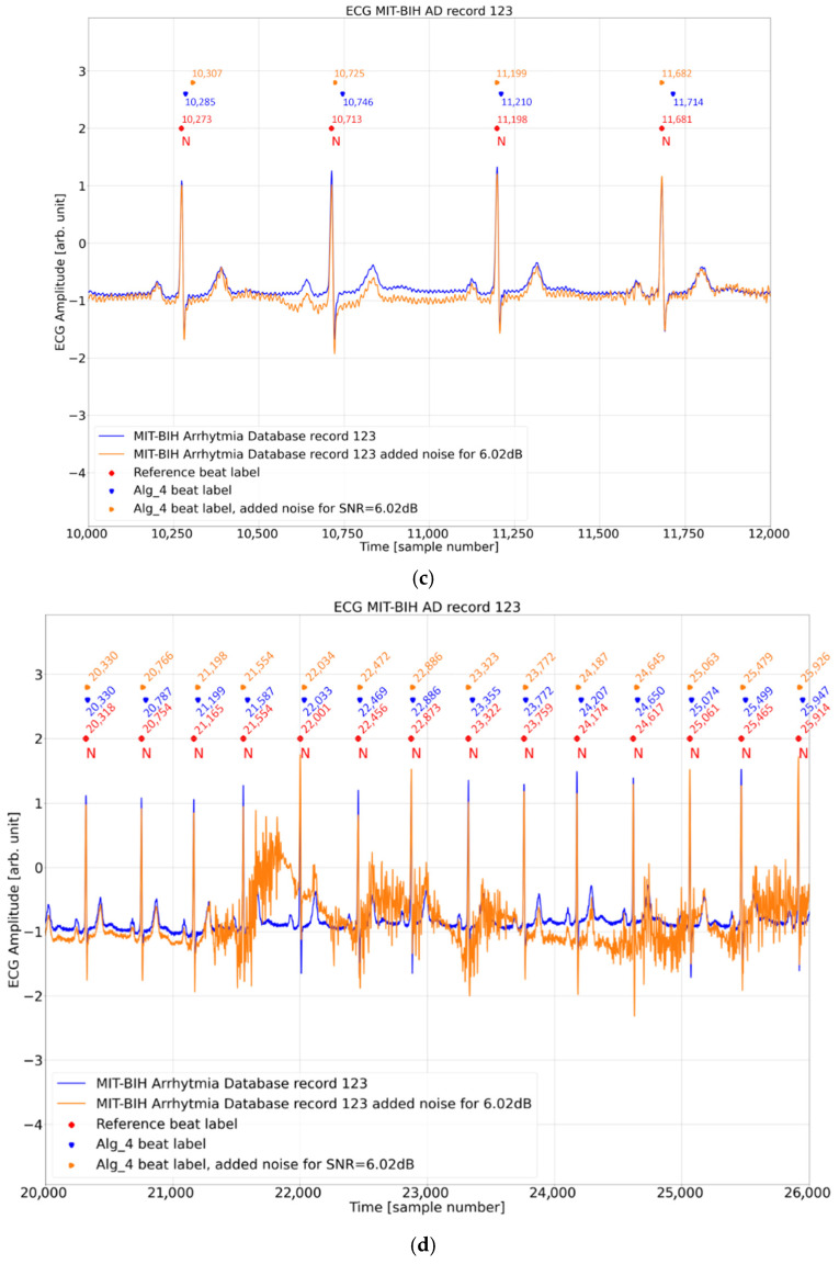 Figure 9
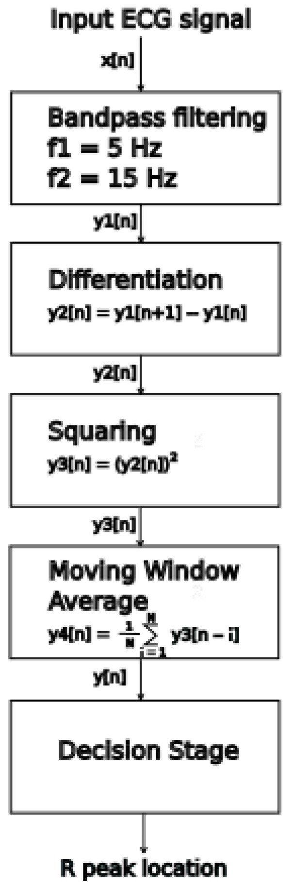 Figure 10
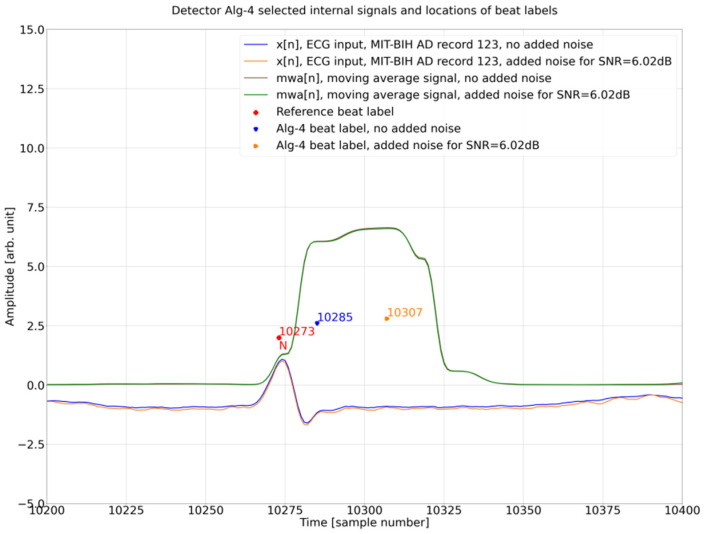 Figure 11
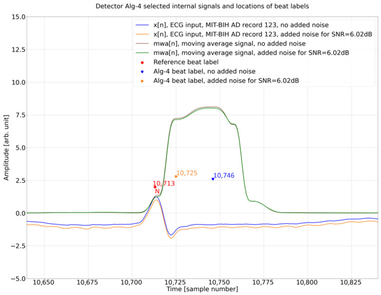 Figure 12
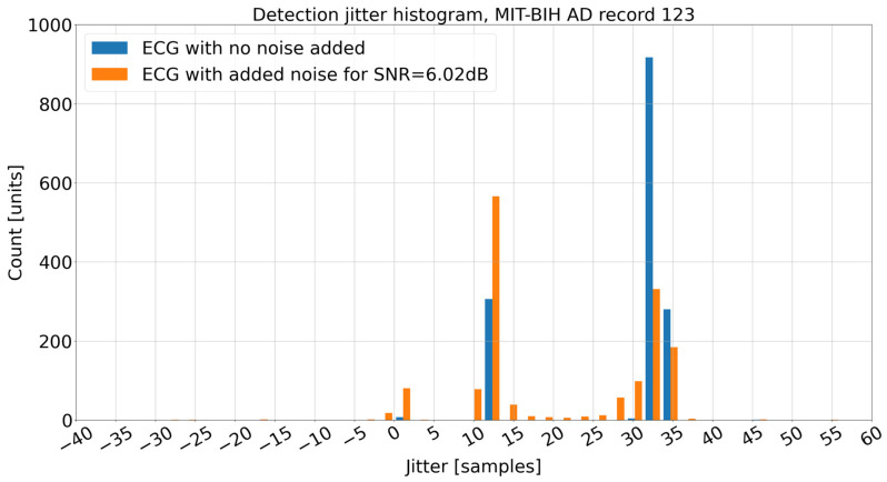 Figure 13
- —AGH University of Krakow
Peer Reviews
No public reviews on file for this paper yet. If you reviewed it on a platform where reviews are public (OpenReview, ICLR, NeurIPS, ICML), you can paste yours below so the community can read it here.
Videos
No videos yet. Explain this paper in a talk, walkthrough, or lecture? Add one.
Taxonomy
TopicsCognitive Radio Networks and Spectrum Sensing · Bluetooth and Wireless Communication Technologies · ECG Monitoring and Analysis
1. Introduction
QRS complex detection is a crucial first processing step in almost any automated ECG analysis [1]. The end result of ECG signal processing includes heart rate determination, heart rate variability determination, heartbeat classification, ECG signal fiducial points determination, on-line patient heart monitoring, and other applications. Hence, the accuracy of QRS detection is of primary importance as any errors from the QRS detection stage will be magnified or propagated to consecutive processing steps negatively influencing the end result of the whole processing chain.
The techniques for automatic QRS detection have been actively developed since the 1950s, and many approaches have been proposed [2,3,4], alongside the techniques for heartbeat classification and automated ECG analysis [5,6,7,8,9,10]. The main difficulties faced by QRS detectors are the wide variety of ECG waveforms, especially in cases of heart disease, and various types of interference present in the ECG signal. There are also technical limitations and considerations influencing the effectiveness of QRS detection: sampling rate, ADC resolution, power consumption considerations (especially important for mobile and wearable ECG acquisition systems) [3,4], hardware platform processing capabilities (especially important for real time operation) [3,4].
Despite the long history of research, only recently, the authors have pointed out that, in addition to the standard statistics of correctly detected QRS complexes, an important feature of the detector is the precision of indicating the temporal location of the detection point, and it is most desirable to maintain high accuracy regardless of the noise level. High temporal precision makes fiducial points directly usable for (1) comparing R-waves in heart beats classification process, (2) calculations of rhythm variability parameters such as HRV and HRT, (3) assessments of S-T segments for ischemia monitoring, and many others. No need for additional resynchronization procedure (such as [11]) is also beneficial to reduce the computational complexity, execution time and power requirements.
In [12], we presented an analysis of the effect of detector time tolerance (DTT) on the detection statistics of QRS complex detectors. In [13], we compared four algorithms, including one of our own, in terms of the sensitivity of their detection statistics for individual heart beat morphologies to gradually increase accuracy requirements in the presence of noise with different signal-to-noise ratios (SNRs). Overall, for all four analyzed detectors, the QRS detection accuracy decreased with increasing noise levels and tightening DTT values. It was also shown that the QRS detection accuracy depends on the heartbeat type and is specific to each detector, with some detectors performing better for a given heartbeat type.
In the current work, our objective was to focus on the specific case of the modern implementation of the Pan Tompkins algorithm [14] available on GitHub version 1.3.5 [15] and described in [13] as Alg-4. Following intuition and fragmentary results obtained in [13], we hypothesize that the temporal stability of detection points (i.e., the reproducibility of detection points at the same locations in QRS complexes of the same type) deteriorates linearly with an increasing noise level (i.e., decreasing SNR). To this end, we increased the density of added noise levels and the expected accuracy of true positive detection. In addition to the comprehensive analysis performed for all records in the ECG database within the DTT range where this influence was greatest, we analyzed individual records’ contributions to change in the total DER. Surprisingly, for some records, adding controlled noise to the ECG signal improves the detection statistics of the Alg-4 algorithm for certain DTT values. We therefore analyzed the step-by-step execution of the algorithm for specific strips of the database record with the greatest influence to pinpoint the computational procedure used in Alg-4 that results in the observed non-linear and non-monotonic relation.
Regarding the specific contribution of the present paper, (1) we stress that applying the temporal tolerance analysis may turn over QRS detectors’ rankings based solely on detection statistics, and (2) we suggest revisiting any research related to temporal ECG parameters (such as HRV) based on inaccurate QRS-detection algorithms.
The remainder of this paper is organized as follows: In Section 2 we will first define benchmarks for detection performance. Then, we will look at known schemes for noise removal and known techniques for correcting the location of the R Peak. We analyze how others rate the influence of noise. With Section 3, we propose a method of how to systematically add artificial noise and what its properties should be. We then, in Section 4, analyze whether there is a monotonic relation between an increase in the noise level and the degradation of detection performance. We will see that this is not always given. As this is a surprising result, we dig for the root cause of this strange behavior. Based on our findings, we propose adjusted criteria for characterizing the detection performance of a QRS detector.
2. Related Work
QRS detection is the first step in automatic ECG analysis; it is followed by additional blocks necessary to achieve the goal of signal processing. This can be HRV parameter analysis, fiducial point determination, heartbeat classification, etc. All blocks and components should fit with each other, and there are many aspects to achieve the goals of ECG signal processing; therefore, we start this section with an overview of classical and new metrics to assess the QRS detection accuracy (and specifically temporal detection accuracy), followed by the following: noise-removal techniques, corrections of R-peak detection points, HRV accuracy, and finally the influence of noise on detection accuracy.
2.1. QRS Detection Benchmarking
The effectiveness of QRS complex detection is typically assessed using a classic binary classification process [2,16]. Reference beat labels (database R peak annotations) are paired with algorithm-produced beat labels (R peaks identified by the algorithm). In order to pair the labels, the maximum time difference between reference the beat label and the algorithm beat label must not exceed a specific time window—the detection time tolerance. In [16], detection time tolerance is specified at 150 ms, whereas in the literature, there are various values: 27.8 ms [17] (ten times sampling period, for MIT-BIH AD [18,19] it is 10 × 2.78 = 27.8 ms) and from 60 ms to 160 ms [12].
Pairing the algorithm’s beat label with the corresponding reference beat label defines binary classification as follows: True Positive (TP): a paired reference beat label and algorithm beat label within the detection time tolerance, False Positive detection (FP): algorithm beat label without a paired reference beat label, False Negative detection (FN): reference beat label without a paired algorithm beat label. The TP, FP, and FN values are then used to calculate the binary classifier metrics: Detection Error Rate (DER), Sensitivity (Se), Positive Predictive Value (PPV), and F1-score (F1), as follows:
where:
FP—False Positive,FN—False Negative,TP—True Positive.
Recently, Porr and Macfarlane [17] proposed a new QRS -detection accuracy benchmarking measure, which integrates the detection time tolerance with the F1-score. They recognized that due to the wide detection time tolerance (for example 150 ms) many QRS-detection algorithms proposed in the literature achieve F1-scores very close to 100%. With small differences in accuracy results, it is not possible to realistically compare and differentiate the proposed QRS-detection techniques. The authors proposed a new benchmarking measure called JF. The process to calculate JF consists of several steps. The first step is the determination of TP_JF_, FP_JF_, and FN_JF_. The pairing for calculating TP_JF_, FP_JF_, and FN_JF_ is performed without a set width window of detection time tolerance. The basis for pairing is not the window of fixed width (for example 150 ms) but proximity; the nearest algorithm beat label and reference beat label are paired. Any unpaired algorithm beat label between two matched pairs is considered FP_JF_, and any unpaired reference beat label between two matched pairs is considered FN_JF_. All matched pairs are counted as TP_JF_. For all TP_JF_ over the database record, the average time distance between reference and algorithm labels is calculated and is called the average temporal jitter . As a next step the average temporal jitter is converted into a performance measure between 0 and 100%:
According to (6), the average temporal jitter of 12 ms will produce a performance measure of 0.5 or 50%. As a next step, the F1JF-score is calculated according to (4) with TP_JF_, FP_JF_, and FN_JF_. Finally, the JF is calculated:
In our opinion, the proposed evaluation JF has a strong point of integrating temporal accuracy. It can be criticized for joining Se and PPV into one metric F1 neglecting that FP and FN have vastly different impacts on the downstream processing chain. It can be solved by defining the JSe and JPPV in an analogous way as F1 is converted into JF.
2.2. Noise Removal
Noise removal is often the first step in the QRS-detection algorithm. The authors in [20] describe the types of noise present in the ECG signal then review existing denoising and preprocessing techniques. Then, they review data transformation and detection techniques and list 15 various ECG signal test databases followed by noise parameters, detection accuracy evaluation parameters. The goal of removing the noise from the ECG signal is to improve the accuracy of QRS detection. As there are many types of noise, the study showed that there is no single technique that is effective for all noise conditions. Also, each denoising operation has some impact (distortion) on the underlying ECG signal. And then, review 38 techniques of QRS detection. In conclusion, the authors state that because modern health care requires wearable devices, only a few from reviewed QRS detection algorithms have been tested in a mobile scenario, a noise and power/complexity requirement.
In [21], the authors define and review six main domains of noise-removal techniques: Empirical Mode Decomposition (EMD), Deep-learning autoencoder models (DAEs), wavelet-based models (WT), Sparsity-based models, Bayesian-filter-based models, Hybrid Models. Describe classification of noise into four types: base-line wander, power-line interference, muscle artefacts, channel noise. The types of noise are described and techniques of removal alongside their performance. In summary, the authors give their assessment of which type of filter is best for which type of noise.
In contrast to numerically complex methods proposed in [21,22], the authors present simple practical digital filter implementation to suppress power grid noise using integer coefficients filters. The proposed filter does not introduce the ECG shape deformations and can be used in power-restricted mobile ECG analysis devices.
2.3. Corrections of R-Peak Detection Points
The temporal accuracy of R-peak detection is of primary importance for HRV analysis. The authors in [23] observed that filtering in the preprocessing stage introduces time lag in the filtered signal, with delay equal to the group-delay of employed filters. Further, they observed that many algorithms set the time location of the R-peak at the maximum amplitude of the filtered signal, resulting in constant per beat slackness. Many QRS-detection algorithms do not provide compensation for this slackness, so the authors propose compensation as a first step to improve QRS-detection accuracy. As a second step to improve the QRS-detection temporal accuracy, the authors propose a process called the Slackness Reduction Algorithm. After locating the approximate location of the R-peak in the filtered signal, the algorithm searches in the original ECG signal for the more accurate location of the R-peak by searching for the highest absolute differential maximum in the vicinity of the maximum found in the filtered signal. The authors evaluated the results of this modification on three algorithms. They found that the average slackness of this algorithms for MIT-BIH AD was 9 ms for normal beats and 13 ms for abnormal beats. With the Slackness Reduction Algorithm, they reduced the average slackness to 4 ms and 7 ms, respectively.
The sampling interval influences the accuracy of the R-peak location necessary for precise HRV measurements. For example, when the ECG signal is sampled with an interval of 8 ms (f_s_ = 125 Hz) without modification, that would be a maximum accuracy of HRV. However, it is still possible to maintain the accuracy of the R-peak location on the level of 1–2 ms for precise heart rhythm measurements with the process proposed in [11]. The author reported that by employing simple calculations (eight multiplications, nine additions, and one division on floating point data) for one R-peak, it is possible to achieve the precision level of 1 to 2 ms. The author employed approximation of the R-wave with the quadratic function with the length of approximation of 32 ms. This way, with little additional computation, it is possible to achieve higher temporal accuracy than the sampling interval.
2.4. Heart Rate Variability
Accurate detection of QRS complexes is essential for reliable HRV computation. In [24], the authors analyze how the QRS-detection accuracy of various QRS detectors impacts the errors in HRV metrics. They analyze the performance of eight QRS detectors on ECG data from the Glasgow University Database (GUDB) [25]. The GUDB contains ECG signals from 25 subjects recorded under five conditions: sitting, walking, performing a math test, using a handbike, and jogging. In addition, each ECG record contains two simultaneously recorded versions, one recorded via elastic chest strap and one with ECG electrodes. The ECG data was therefore recorded under vastly different levels of noise and artifacts. The 23 HRV metrics were computed based on the outputs from eight QRS detectors and compared with HRV metrics computed based on database annotations. The results show that some detectors perform better than others and none is the best for all tested conditions. Another result is that the relationship between the QRS-detection accuracy and HRV accuracy is metric-dependent and nonlinear. In summary, the authors call for further research to investigate the impact of signal processing and RR interval correction techniques to further improve the robustness of HRV calculations in real-life noisy settings.
In [26], the authors analyzed the performance of a Modular Analysis System (MEANS) to assess its accuracy in heartbeat classification and to study the effects of undetected non-sinus heart beats on HRV parameters. The ECG data used in the study consisted of 20 min ECG records from 1674 patients from the CARLA study (CARdiovascular disease, Living and Ageing in Halle). The heartbeat classification was performed, into three categories: normal sinus rhythm, supraventricular systoles, ventricular systoles. The MEANS system correctly classified 99% of all beats in the study. Compared to reference data, the MEANS system gave a higher SDNN on average (4.9%), and other HRV parameters were also overestimated (from 6.5% to 29%). On the other hand, the results from MEANS did not substantially change the association of HRV and CVD risk factors. The authors also observed that one or few misclassified N-type heartbeats mean large changes in HRV values; at the same time, many false N-type heartbeats lead to small effects on the HRV. In summary, the authors see the need for further improvements in detecting supraventricular systoles or alternatively an indication of the difficulty for algorithmic analysis stretches of the ECG that must have an additional visual reading.
The critical influence of the QRS-detection accuracy on HRV calculations is analyzed in [27]. The analysis was performed on all RR intervals (for simplification all RR intervals were taken instead of the standard approach with only NN intervals) using all MIT-BIH AD records with various added levels of artificial accuracy error. The time domain, frequency domain, and selected nonlinear HRV parameters were calculated (in total 12 parameters) for each added accuracy error. The results show that, in general, time domain parameters are resistant to accuracy error with HRV parameter error values from 1.3% to 0.02% for accuracy error σ = 8 ms and with the exception of pRR50 with an error of 15% for same accuracy error, whereas frequency parameters exhibited errors from 38% to 55% for σ = 8 ms. The selected nonlinear HRV parameters are from 0.83% to 7.5%. In summary, the authors express the opinion that the results of HRV depend strongly on many conditions: sampling frequency, type of QRS detector used, QRS classification procedure, ECG device model, type of heart disease (as low variability of time series and arrhythmic behavior will influence the total HRV error).
2.5. Analysis of Noise Influence on Detection Accuracy
In [28], the authors analyze the influence of noise on nine different QRS-detection algorithms, which they selected based on low complexity and high performance. Low complexity criteria were that the algorithm could be run on an 8-bit microprocessor, and with high performance criteria, the authors rejected algorithms with poor accuracy performance for input ECG signals with low noise levels. The algorithms were published from 1971 to 1983. The algorithms were as follows: (1) based on amplitude and first derivative: Moriet-Mahoudeaux, Fraden-Neuman, Gustafson, (2) based on first derivative only: Menard, Holsinger, (3) based on first and second derivative: Balda, Ahlstom-Tompkins, (4) based on digital filters: Engelsee-Zeelenberg, Okada. The ECG signal noise sources identified by the authors were as follows: electromyografic, 60 Hz powerline, baseline drift due to respiration, abrupt baseline drift, and composite noise constructed from the mentioned noise sources. The authors created ECG signals with added simulated noise added to the uncorrupted ECG signal at four levels: 25, 50, 75, and 100% of the maximum amplitude. They adopted 88 ms as temporal time tolerance for the TP/FP/FN determination. The authors also measured and reported the changes in detection delay with an increased level of input noise. In summary, the authors stated that noise deteriorated the accuracy of the algorithms and there was no one best algorithm that was superior for all types of noise considered in their study. For electromyografic noise, the best performance was exhibited by algorithms based on the slope and amplitude. For composite noise, the best performance was recorded for algorithms based on digital filters.
The influence of noise on the accuracy of three well-known algorithms was analyzed in [29]: Pan-Tompkins, WQRS, and Hamilton. Algorithm selection criteria were as follows: real time operation and robust performance with input ECG noise. The authors evaluated TP, FN, FP, Se, and PPV on records from MIT-BIH AD with different levels of added noise coming from baseline wander (BA), muscle artifact (MA), and electrode motion (EM). Noise data was from the MIT-BIH Noise Stress Test Database. The level of input ECG signal added noise was from −12 dB to 12 dB with a step of 3 dB. The three algorithms showed similar accuracy results expressed in Se and PPV with an input signal with no added noise. The accuracy deteriorated with added noise and for all 48 MIT-BIH records for SNR = −12dB, the results reported by the authors were respectively for Pan-Tompkins, WQRS, and Hamilton:
- BW noise: Se: 99.42%, 94.58%, 98.13%; PPV: 97.21%, 62.45%, 95.74%
- MA noise: Se: 85.94%, 84.71%, 81.74%; PPV: 59.68%, 36.95%, 61.74%
- EM noise: Se: 68.85%, 65.44%, 84.10%; PPV: 42.54, 33.09%, 44.05%
Is summary, the authors observed that added composite noise at −12 dB significantly degraded all analyzed algorithms’ accuracy expressed in Se and PPV. In detail, the EM had the highest influence on the detection accuracy, followed by MA and BW. The detection temporal tolerance was not specified by the authors, which makes comparisons to other works difficult.
In [30], the authors proposed an R-peak-detection algorithm based on Hilbert transform and evaluated the algorithm accuracy results Se, PP, and DER achieved with ECG signals contaminated with noise. The ECG signals from MIT-BIH NSTD were prepared with five SNR values from 24 dB to 0 dB with a 6 dB step. The authors compared the results with four detectors known from the literature (Pangerec U. et al., Antink C.H. et al., De Cooman T. et al., Vollmer M.) achieving similar or better results. The detection temporal tolerance adopted by the authors was 150 ms. The results of the proposed QRS-detection method show that up to SNR = 6 dB, the influence of noise on the detection accuracy is minimal with Se = 98.13% and PPV = 96.91%, whereas for SNR = 0 dB, the accuracy deteriorates significantly to Se = 78.98% and PPV = 75.25%.
The influence of the noise, detection temporal tolerance (DTT), and QRS morphology on QRS-detection accuracy was analyzed in [13]. The authors analyzed four QRS detectors known from the literature (Gutiérrez-Rivas R. et al., Reklewski W. et al., Ravanshad, N. et al., Pan-Tompkins). To measure the changes in the QRS-detection accuracy, a scaled amount of MA noise (four levels) was added to MIT-BIH AD records, and the influences of six QRS morphologies and five values of DTT were analyzed. The detection accuracy, expressed as a ratio of True Positive/Total Beats (TP/TB), generally deteriorated with added levels of noise and decreasing values of detection temporal tolerance. For one detector (Pan-Tompkins), there was an unexpected improvement with added levels of noise for certain values of DTT. In terms of the influence of the QRS morphology on detection accuracy, the most difficult for accurate QRS detection was V-type (Ventricular beats) for three algorithms and L-type (Left bundle branch block beat) for one algorithm under study. The average (across all DTT and QRS morphologies) detection accuracy results expressed as the True Positive/True Negative ratio (TP/TB) for algorithms under analysis were respectively 83.72% to 82.17%, 90.68% to 89.18%, 77.12% to 71.74%, and 62.03% to 70.32% for levels of noise increasing from SNR = “no noise added” to SNR = 3 dB. As mentioned earlier, for the Pan-Tomkins algorithm, there was an improvement observed in TP/TB with added noise levels from 62.03% to 70.32%.
3. Materials and Methods
In order to analyze the effects of improving and worsening the DER (Equation (1)) with increasing levels of noise and a reduction in the detection tolerance time (DTT) on the QRS detector accuracy we have tested algorithm Alg-4 from [13] (Porr algorithm). The tests are carried out for a range of DTT values and a range of controlled added muscular noise achieved by mixing muscular noise patterns with MIT-BIH AD records (Figure 1).
First, we reproduced detection accuracy obtained in [13] and expressed it as TP/TB. Next we extended the analysis from [13] with more levels of added noise, expressed as SNR, and conducted the calculations for the same DTT range as in [13] but with larger number of DTT values in order to reduce result graininess. We switched from measuring the QRS-detection accuracy as the TP/TB ratio to DER as it is a more universally employed measure. The TP/TB and DER values here are totals for all 48 MIT-BIH AD records.
To study the influence of an added controlled level of noise to the ECG input signal, we applied a test data set consisting of modified ECG signals from MIT-BIH AD with an added noise signal from MIT-BIH NTSD, a muscle artifact record (MA). We have used all 48 original MIT-BIH AD records, which contain intrinsic noise, and thus, our analysis starts from SNR with an “original” level of noise and not a noise-free ECG record. The added level of SNR has been calculated based on the average power factor of the original record and added noise pattern. The calculation method is described below in the Noise source and mixing section.
The algorithm is tested on the MIT-BIH Arrhythmia Database (MIT-BIH AD) with added muscular noise from the MIT-BIH Noise Stress Test Database (MIT-BIH NSTD) [31]. The tests were conducted on a Dell Latitude E6400, Intel Core2Duo P8400, 2.26 GHz, and 4 GB RAM running with Debian 10.13. Implementation of the algorithms, test tools, and data processing was performed in Python 3.11.2. Plots were created in Jupyter Notebook (server v6.4.12 with Python 3.11.2 [GCC 12.2.0]).
3.1. QRS-Detection Algorithm
Algorithm Alg-4 [13] (Porr algorithm) is an implementation of the Pan Tompkins algorithm. It was selected as a study case because of being the most often cited reference algorithm originating from 1985. The original algorithm preprocessing chain consisting of band pass filtering, differentiation, squaring, and the window moving average is retained as the ‘feature function’. The feature function is further analyzed to find local extrema. When a given local extrema surpasses the threshold value, then the local extrema becomes the algorithm R-peak detection and the algorithm enters a 300 ms waiting state, as it is not possible physiologically for the next R-peak to occur within 200 ms; this implementation extends this waiting state to 300 ms. After the pause, the algorithm resumes the local extrema search and comparisons with the threshold value. The searchback mechanism, a adjustment of the threshold value based on regular and irregular heart rates, is implemented.
3.2. Detection Time Tolerance Range
The range of acceptable tolerance (DTT) tested in this work is presented in Table 1.
3.3. Noise Source and Mixing
In order to prepare versions of test ECG records with various levels of noise, we have used the upper channel signal from the MIT-BIH AD and added a noise signal from the MIT-BIH NSTD [31] multiplied by adequate scaling factors. For wearable applications and due to the omnipresence of muscle artifacts, we decided to use a “muscle artifact” (MA) record from the MIT BIH NSTD. According to physionet.org, MIT-BIH NSTD is a database related to MIT-BIH AD and includes 12 half-hour ECG recordings and 3 half-hour recordings of noise typical in ambulatory ECG recordings [31]. The three noise records were assembled from the recordings by selecting intervals that contained predominantly baseline wander (in record ‘bw’), muscle (EMG) artifact (in record ‘ma’), and electrode motion artifact (in record ‘em’) [31].
The records from MIT-BIH AD and MIT-BIH NSTD were captured with the same sampling parameters and have the same length. We have used original records from the MIT-BIH AD, and the intrinsic noise is already present in the data and is out of our control. Consequently, mixing additional noise creates a record with additional noise added on top of already existing noise in the particular record. So this will be called the relative signal-to-noise ratio (SNR). The relative SNR can be calculated based on the root mean square (RMS) of the original record RMSs (MIT-BIH AD) and added noise pattern RMSn (MIT-BIH NTSD record MA).
where:
xs_i_—a record from MIT-BIH AD, signal valuesxn_i_—MA record from MIT-BIH NSTD, noise values —root mean square amplitude of signal —root mean square amplitude of noise
The levels of noise mixing (SNR) tested in this work are presented in Table 2.
The following procedure has been employed to achieve target relative SNR levels as listed in Table 2. In the first step, the RMSs for one selected record from MIT-BIH AD and RMSn for the MA record from MIT-BIH NSTD are calculated according to Equations (8) and (9). Next, we can rewrite Equation (7) to express the required target RMS as tRMS as in Equation (10). In the next step, the scaling factor m is calculated. And the last step includes preparing the record with the required target SNR value according to Equation (12).
where:
m—scaling factor —target SNR
where:
ECG—original ECG record from MIT-BIH AD e.g., record 100MA—MA record from MIT-BIH NTSD
The above presented noise-mixing procedure is repeated for all 48 records from the MIT-BIH AD database and for all 18 target noise levels of values specified in Table 2. This produced a total of 864 half-hour test files used to determine the Detection Error Rate that is the main goal of the experiment.
3.4. Individual ECG Record Analysis
Typically, the MIT-BIH AD is used as a collection of typical ECG recordings with specific characteristics representing the true-to-life occurrence of individual heartbeat types. In addition to the global, statistical approach, we also analyzed the impact of individual records on the overall DER value. This allowed us to identify cases particularly sensitive to noise and the tight temporal tolerance of detection points.
4. Results
This section presents the results of DER calculated for the whole collection of 48 MIT-BIH AD files in the full range of the noise level, initially for the full range of DTT and next narrowed to the range where the DTT curve is the steepest representing the fastest drop of detector performance (Section 4.1). Next, we limit the range of considered noise levels and seek a performance drop file-by-file to detect the MIT-BIH AD record where the detector performance drop is the fastest (Section 4.2). Surprisingly we also found files in which the presence of noise improves detection statistics, in particular file 123 (Section 4.3). Finally, we focused on selected ECG strips in this file to find the reason for this unexpected result.
4.1. General Performance of the Detector Under Test
For each DTT and SNR pair, the aggregate detection efficiency (expressed by TB, TP, FN, FP, and DER) is calculated for 48 records from the MIT BIH AD database (Figure 2 and Figure 3).
Figure 4 displays magnification of Figure 3 within the range of detection temporaltolerance (DTT) of 35 to 31 samples (corresponding to 97.23 ms and 86.12 ms), where the detector’s performance statistics drop dramatically.
The DER results for individual MIT-BIH AD records for DTT = 59, 35, 31, and 3 samples for no noise added and added noise for SNR = 6.02 dB are listed in Table A1, Table A2, Table A3 and Table A4 in the Appendix A.
4.2. Identification of Most Contributing ECG Files
Observing the results in Section 4.1, summarized in Table 3, we asked the following question: which of the 48 MIT-BIH AD records contribute the most to the changes in the total DER shown in Figure 3 and Figure 4? Research for an answer led us to study individual record contributions. For this study, we limited the noise level to two values: the “no added noise” (signal number 1 in Table 2) and the noise-added version of input signal (signal number 10 in Table 2), for added noise up to SNR = 6.02 dB. Results of the study are presented in Figure 5.
Consequently, we indicated records for which the difference in results without adding noise and after adding noise to SNR = 6.02 dB for fixed DTT = 31 and then for fixed DTT = 35 was the most important (Figure 6). Moreover, we indicated records for which the change in DER after moving from DTT = 35 to DTT = 31 at a constant SNR is the most significant (Figure 7). In Figure 7, it can be seen that the biggest differences in DER are for 115, 123, and 109 for both studied SNR levels (no added noise and noise up to 6.02 dB).
In Figure 6, it can be seen that the input signal with added noise improves the results the most for record 123 (the difference in DER is approximately +85), followed by record 219 (the difference in DER is approximately +70), and then records 115, 109, and 102. At the same time, it can be observed that for two records, the signal with added noise causes a significant deterioration in the DER result: for 121 (the difference in DER is approximately −70) and 117 (approximately −60). A decrease in detector performance with a growing noise level was somewhat expected; however, the opposite case is worth further studies. To this point, record 123 will be investigated to find a plausible reason for the improvement in the DER after adding noise.
4.3. Fiducial Points Instability in File 123
Surprisingly, adding noise may improve the fiducial points stability (i.e., reduce DER). In file 123, it can be observed that for the input ECG signal without added noise, some of the algorithm’s detection points are shifted by approximately 30 samples. Annotations from the MIT BIH AD database for time values on the x-axis are equal to the following:
- 70 samples (115 − 70 = 45 samples of shift),
- 1498 samples (1531 − 1498 = 33 samples of shift),
- 8892 samples (8925 − 8892 = 33 samples of shift),
- 9326 samples (9359 − 9326 = 33 samples),
- 9793 samples (9827 − 9793 = 34 samples),
- 10,273 samples (10,285 − 10,273 = 12 samples),
Figure 8a–d show detailed fiducial point timing in these particular strips of the 123 record.
4.4. Internal Operation Analysis
To shed light on the background of this surprising result (Section 4.3, see particularly Figure 8c with a relatively clean ECG), we analyzed, in greater detail, the Porr algorithm (Figure 9) internal operation for two detections related to database annotation at sample 10,273 and 10,713 for the ECG input signal with no added noise and added noise for SNR = 6.02 dB. For the reference beat label at 10,273, algorithm detection for the ECG input signal with no noise added at 10,285 is close to the annotation with a delay of 12 samples, whereas for the reference beat label at the 10,713 algorithm detection for the ECG input signal with no noise added at 10,725, it is close to the annotation with a delay of 12 samples (Figure 8c). These two beats represent the two opposing results and are thus the subject of further analysis. As can be seen in Figure 10, in this excerpt, there are three cases (detections 2, 3, 4) where the Porr algorithm beat labels for the input ECG signal with added noise are closer to the reference beat label than the beat labels for the input ECG signal with no noise added and one case where detection for no added noise is closer to the reference beat label.
Further analysis is presented in Figure 10 and Figure 11, below which an additional signal is presented, the output of the Porr algorithm preprocessing stage—Moving Window Average—mwa[n] signal.
When comparing Figure 10 and Figure 11 it can be noted that in both of these figures, the mwa[n] feature signal (final preprocessing signal before decision stage) looks very similar between the figures and between the two versions of the ECG input signal—the one without added noise (brown line) and the one with added noise (green line). At the same time, the order of algorithm beat labels versus the reference beat label in both figures is different. In Figure 10 the beat label for the input signal without noise is closer to the reference beat label, whereas in Figure 11, the beat label for the input signal with added noise is closer to the reference beat label.
To find out why it is a case, we have analyzed the decision stage in the Porr algorithm. There are two crucial moments:
- finding the peak in the mwa[n] signal,
- checking if the mwa[n] signal value at the found peak is greater than the algorithm detection threshold
The above operations are conducted in the below instructions: Instruction (2) is looking for local maxima in the mwa[n] signal; this is performed for all samples in the ECG record, Instruction (1). Next, for each local maxima found called a ‘peak’, the condition is checked if the signal mwa[n] at the peak is greater than threshold_I1 and if the previously found R peak was more than 108 samples (300 ms) earlier, the refractory condition. If that is true, then, the location found is assigned the algorithm beat label (Algorithm 1). Algorithm 1. Porr algorithm snippet performing peak detection.for i in range (1, lenght_of_ECG_record): (1) if mwa[i-1] < mwa[i] and mwa[i + 1]<mwa[i]: # if True -> peak is detected (2) if mwa [i] > threshold_I1 and (peak-signal_peaks[−1]) > 0.3·fs: (3) # second condition checks if previous # peak is more than 108 samples # earlier (300 ms refractory blanking). # if True -> peak is R peak (algorithm # label)# if False -> peak is a noise peak
Analyzing, in detail, Table 4 in connection with Figure 10, it can be noted that the algorithm-detection delay is smaller for the ECG input signal with no added noise as compared to noise added. This situation can also be observed in the Figure 8b database reference at sample number = 8409, the algorithm beat label for no added noise at 8421, and added noise of 6.02 dB at 8442 and in the Figure 8c database reference at 10,273, algorithm beat label for no added noise at 10,285, and added noise of 6.02 dB at 10,307.
Analyzing, in detail, Table 5 in connection with Figure 11, it can be noted that the algorithm-detection delay is smaller for the ECG input signal with added noise as compared to no noise added. This situation can also be observed in the Figure 8b database reference at sample number 8892 and Figure 8c database reference at sample number 10,713, 11,198, and 11,681.
5. Discussion
A regular QRS detector with large jitter of detection points needs additional procedures to center (i.e., synchronize) the QRS waves e.g., parabola fitting. The purpose is twofold: (1) provide a fiducial point to start time-based calculations of parameters (such as HRV) or amplitude measurement points (such as ST slope) and (2) provide a reference for a cross-correlation-based comparison of signals (for clustering and classification). Two approaches have been presented in the literature: either such centering was performed and precise R-points were calculated at the cost of additional computational load, or the centering was omitted saving machine cycles at the cost of parameters of only approximate quality. Our paper identifies another alternative: having a low complexity low jitter QRS detector robust to noise. In particular, the presence of noise together with low power requirements is typical for wearables; our findings may thus be of particular interest in pursuit for high quality ECG parameters from wearables.
The results obtained show that for almost all SNR values, when the DTT value is reduced from DTT = 97.23 ms to DTT = 86.12 ms (i.e., from DTT = 35 to DTT = 31 samples), there is a sharp drop in performance (i.e., rise of total DER) for all 48 MIT-BIH AD records. This is an interesting novelty in the methodology, because it would allow the detector to be examined as a black box, i.e., without knowledge of its structure. Regarding the detector under test, a delay (inaccuracy of the ‘R’ reading) of 80–100 ms is quite significant. The largest drop in the value of DER was observed for two SNR values: SNR = ‘no added noise’ and SNR = 6.02 dB (ratio of average amplitudes , i.e., the average amplitude of the useful signal is 2 times greater than the added noise). The amount of delay of this particular algorithm suggests that fiducial points, being its results, should rather be corrected before use in time-related ECG procedures. This statements challenges many papers in which the authors use the QRS-detection series directly for calculations of HRV, heart beat classifications, or estimations of the S-T segment.
In [32], we proposed a multiplierless QRS detector working fast (i.e., with minimum computational burden), precisely (i.e., with excellent detection statistics), and with far less delay (i.e., maintaining good results with less tolerant assumptions). We compared it to several other low-delay QRS detection methods developed recently.
In this paper, we examined the most popular implementation of the most popular QRS-detection algorithm, developed by Pan Tompkins [14], implemented by [15] and available on GitHub. Based on citation statistics, this implementation is considered the most frequently used as a ‘black box’ by the developers of ECG algorithms with a wide range of complexity. To shed more light on the implementation quality, we examined it, applying more true-to-life signal conditions and possibly more thoroughly than anyone previously, using the most accessible database of MIT-BIH AD records [19,20].
First, we generated regular statistics of detection performance (incl. Acc, PPV, DER etc.).Next, we examined how detection-performance statistics decrease with increasing timing accuracy requirements by narrowing the range of temporal tolerance (DTT), i.e., allowed time between detection and reference points. We concluded that this algorithm’s results are not directly applicable for time series analyses of ECG, such as HRV, QT, S-T, etc.Further, we examined how increased noise levels affect the stability of the detection point. We found that, as expected, in most cases, higher noise levels lead to greater inaccuracies. However, we also observed situations (files: 123, 219, 115, 109, and 102) where higher noise levels resulted in improved detection statistics.We found several outlying cases and further seek the file in which this surprising situation was most pronounced. For selected ECG segments in file 123, we analyzed the algorithm’s execution step by step. We concluded that the source of the unexpected behavior is the ambiguous implementation of the local maximum definition applied to the feature function.
The observed phenomena of DER improvement based on the ECG input signal with added noise for SNR = 6.02 dB are caused by the local maximum detection mechanism used in the Decision Stage (Figure 9). The local maximum that is a candidate for the R break is searched in the mwa[n] signal. In idealized relationship [33] between the QRS complex and mwa[n] signal, the R peak, occurs approximately in the middle of the rising slope of mwa[n] (Figure 10 and Figure 11) (the time shift noticeable in Figure 10 and Figure 11 is due to group delay of the bandpass filter and a delay in differentiation and moving window average operations, Figure 9). In theory, the Porr algorithm is supposed to detect the first peak as soon as the rising slope ends (Figure 10 and Figure 11). In practice, due to the requirement for the local peak, the preceding and following samples have to have lower values, and considering that the mwa[n] signal is the time-averaged signal over 54 samples (150 ms), this condition for the local peak is often not met around the beginning of the plateau, and the detection of the peak often occurs later during or at the end of the plateau of the mwa[n] signal. This delay has been observed in this work to be about 33 samples (approx. 92 ms), which is a significant number and can be observed in Figure 12. Adding noise for SNR = 6.02 dB reduces the detection jitter by moving a significant number of detections to about 13 samples (approx. 36 ms); this can be observed in the histogram in Figure 12.
Adding noise increases variability of the mwa[n] signal, which often results in earlier detection of the local extrema, reducing the jitter, as has been observed in Figure 11 and Table 5, which in turn translates to improved DER results for a given DTT. Of course, for the tested algorithm, the DER is already poor at DTT = 31 samples (Table A3), but the fact still remains that the DER for the added noise of 6.02 dB is lower than the DER for no added noise for DTT = 31 and lower values of DTT.
Our research points out that Pan Tompkins as the QRS-detector reference has a limitation not described in the existing literature. Current detectors are compared with a flawed reference; then, the comparison is meaningless, and science is not advanced. Despite better results, we do not find a better commonly used reference in the literature. Moreover, in different variants, the Pan Tompkins algorithm is widely used as a front-end black-box procedure by researchers investigating further steps of the ECG-processing chain.
Results of this paper are potentially interesting as an example of detailed testing of the QRS-detector procedure, where most authors only provide selected detection statistics (DER, PPV, Se without DTT, and statistics noise resistance). Both [13] and [17] are consistent in showing that most detectors are converging to 100% accuracy if DTT is large enough (i.e., inaccurate pairing is allowed). Our results may also motivate one to revisit other papers focused on further steps of ECG processing, with a carelessly implemented flawed version of the reference QRS detector (Pan Tompkins) as a black-box ready-to-use procedure.
It is worth a remark that an imprecise definition of the local maximum was already noticed in an early improvement of the Pan Tompkins [14] algorithm, known as the Hamilton Tompkins method [33]. In the algorithm implementation selected in our study, the local peak was searched in the moving average signal (mwa[n]) with a series of if–then conditions and depending on the expected signal properties (sample to sample value changes), which are not met, thus omitting the maximum at its true position. The conclusion from our research is much more general and does not apply only to the Alg. 4 detector. Thorough testing of the detector (and virtually any kind of medical interpretive software) in any imaginable conditions helps in revealing software faults of which the effects are rarely revealed but medically important.
6. Conclusions
Our research clearly indicates that selecting a QRS-detection algorithm based solely on detection statistics may lead to incorrect results. A significant parameter is the change in statistics as the requirements for the temporal accuracy of the detection point change. Algorithms that maintain high true positive detection statistics, even within narrow time tolerances, enable direct application of their results to time-based ECG analyses such as HRV. Algorithms for which statistics deteriorate rapidly require the use of centering procedures to stabilize the QRS-detection point locations. Another important parameter is the robustness of the detection statistics and the temporal stability of the detection point to noise level variations. Long-term electrocardiogram recordings in normal human life are typically accompanied by variable muscle activity and the influence of external electromagnetic fields, so the QRS detector’s immunity to interference fluctuations is highly desirable.
The reference list from the paper itself. Each links out to its DOI / PubMed record.
- 1Sörnmo L. Laguna P. Bioelectrical Signal Processing in Cardiac and Neurological Applications Academic Press New York, NY, USA 2005
- 2Kohler B.-U. Hennig C. Orglmeister R. The principles of software QRS detection IEEE Eng. Med. Biol. Mag.200221425710.1109/51.99319311935987 · doi ↗ · pubmed ↗
- 3Elgendi M. Eskofier B. Dokos S. Abbott D. Revisiting QRS detection methodologies for portable, wearable, battery-operated and wireless ECG systems P Lo S ONE 20149 e 8401810.1371/journal.pone.008401824409290 PMC 3883654 · doi ↗ · pubmed ↗
- 4Wang R. Veera S.C.M. Asan O. Liao T. A Systematic Review on the Use of Consumer-Based ECG Wearables on Cardiac Health Monitoring IEEE J. Biomed. Health Inform.2024286525653710.1109/JBHI.2024.345602839240746 · doi ↗ · pubmed ↗
- 5Berkaya S.K. Uysal A.K. Gunal E.S. Ergin S. Gunal S. Gulmezoglu M.B. A survey on ECG analysis Biomed. Signal Process. Control 20184321623510.1016/j.bspc.2018.03.003 · doi ↗
- 6Luz E.J.D.S. Schwartz W.R. Cámara-Chávez G. Menotti D. ECG-based heartbeat classification for arrhythmia detection: A survey Comput. Methods Programs Biomed.201612714416410.1016/j.cmpb.2015.12.00826775139 · doi ↗ · pubmed ↗
- 7Boulif A. Ananou B. Ouladsine M. Delliaux S. A literature review: ECG-based models for arrhythmia di-agnosis using artificial intelligence techniques Bioinform. Biol. Insights 2023171177932222114960010.1177/1177932222114960036798080 PMC 9926384 · doi ↗ · pubmed ↗
- 8Gour A. Gupta M. Wadhvani R. Shukla S. Ecg based heart disease classification: Advancement and review of techniques Procedia Comput. Sci.20242351634164810.1016/j.procs.2024.04.155 · doi ↗