Free-energy perturbation in the exchange-correlation space accelerated by machine learning: application to silica polymorphs
Axel Forslund, Jong Hyun Jung, Yuji Ikeda, Blazej Grabowski

TL;DR
This paper introduces a machine learning method to improve predictions of phase transitions in silica using advanced computational techniques.
Contribution
The novel contribution is a machine-learning-accelerated free-energy-perturbation method for evaluating exchange-correlation functionals.
Findings
Machine learning improves accuracy in predicting transition temperatures for silica polymorphs.
Only fifth-rung functionals achieve less than 5% relative error in temperature predictions.
The method provides a framework for evaluating and developing new functionals.
Abstract
We propose a free-energy-perturbation approach accelerated by machine-learning potentials to efficiently compute transition temperatures and entropies for all rungs of Jacob’s ladder. We apply the approach to the dynamically stabilized phases of SiO2, which are characterized by challengingly small transition entropies. All investigated functionals from rungs 1–4 fail to predict an accurate transition temperature by 25–200%. Only by ascending to the fifth rung, within the random phase approximation, an accurate prediction is possible, giving a relative error of 5%. We provide a clear-cut procedure and relevant data to the community for, e.g., developing and evaluating new functionals.
Genes, proteins, chemicals, diseases, species, mutations and cell lines named across the full text — each resolved to its canonical identifier and authoritative record.
Click any figure to enlarge with its caption.
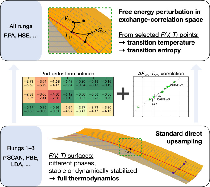 Figure 1
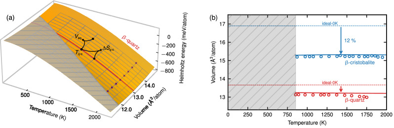 Figure 2
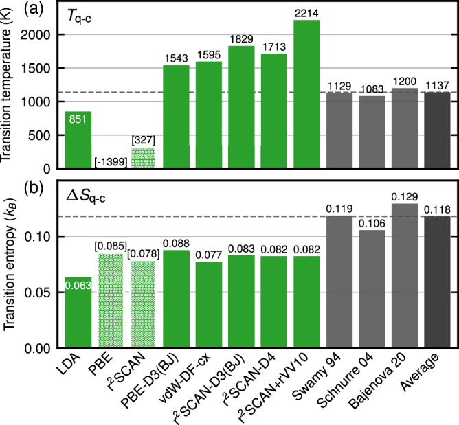 Figure 3
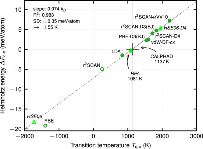 Figure 4
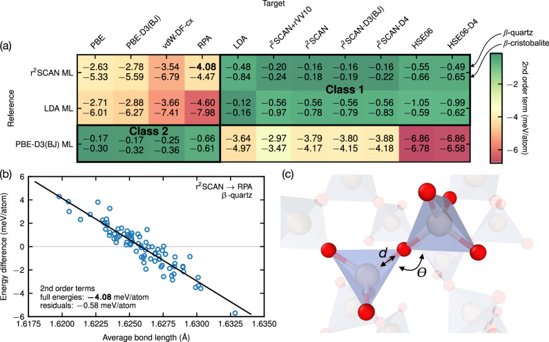 Figure 5
- —https://doi.org/10.13039/501100001659Deutsche Forschungsgemeinschaft
- —https://doi.org/10.13039/501100000781European Research Council
- —Erlangen National High-Performance Computing Center
Peer Reviews
No public reviews on file for this paper yet. If you reviewed it on a platform where reviews are public (OpenReview, ICLR, NeurIPS, ICML), you can paste yours below so the community can read it here.
Videos
No videos yet. Explain this paper in a talk, walkthrough, or lecture? Add one.
Taxonomy
TopicsMachine Learning in Materials Science · Material Dynamics and Properties · Phase Equilibria and Thermodynamics
Introduction
The search for the ultimate exchange-correlation functional in density functional theory (DFT) is the most significant challenge for first-principles calculations in materials science. The flora of approximations was divided into rungs on Jacob’s ladder by Perdew and Schmidt^1,2^. Starting from the local density and generalized gradient approximation (LDA and GGA), the sophistication increases up to the highest chemical accuracy. At the top resides the random phase approximation (RPA), which considers exact exchange together with an approximate many-body treatment of correlations^3–7^. Being nonlocal, the latter also effectively includes dispersion interactions, while, for lower rungs, semiempirical dispersion corrections may be required. Despite the increased sophistication, the higher-level approximations do not always lead to improved results^8–10^. Evaluation against experiments is thus critical and has, conventionally, been performed for 0-K properties such as lattice constants and cohesive energies^8–21^, see Table 1. In a few cases, low-temperature approximations were used^22^, which, however, can lead to errors at elevated temperatures^23^. Even worse, dynamically unstable phases, such as titanium alloys, high entropy alloys, certain perovskites, and silica, cannot be treated at all.Table 1. Ab initio studies evaluating the performance of the exchange-correlation treatment (mGGA=meta-GGA, hGGA=hybrid GGA; 0 K equilibrium properties: a0=lattice constant, B=bulk modulus, Ecoh=cohesion energy, Eform=formation energy; finite temperature (T) properties: Tq−c=transition temperature between β-quartz and β-cristobalite in SiO_2_, \documentclass[12pt]{minimal} \usepackage{amsmath} \usepackage{wasysym} \usepackage{amsfonts} \usepackage{amssymb} \usepackage{amsbsy} \usepackage{mathrsfs} \usepackage{upgreek} \setlength{\oddsidemargin}{-69pt} \begin{document}$${\bf{\Delta}}$$\end{document} Sq−c=corresponding transition entropy)LDAGGAmGGAhGGARPAYearRef.PropertiesRung →12345No. of solids2003^11^a0, B0 Kxxx182009^12^a0, E_coh_0 Kxxx362009^13^a0, B0 Kxxx602011^14^a0, E_coh/form_0 Kxxx302011^15^a0, E_coh_0 Kxxx202013^8^a0, E_coh_0 Kxxx302013^9^a0, B0 Kxxxxx62014^17^E_coh_0 Kxxxx202015^18^a_0_0 Kxxx202016^10^a0, Ecoh, B0 Kxxxx492018^19^a0, E_form_0 Kxx2002022^20^a0, E_form_0 Kxx60002023^21^a0, Eform_0 Kxx1000This workfinite T, Tq−c, \documentclass[12pt]{minimal} \usepackage{amsmath} \usepackage{wasysym} \usepackage{amsfonts} \usepackage{amssymb} \usepackage{amsbsy} \usepackage{mathrsfs} \usepackage{upgreek} \setlength{\oddsidemargin}{-69pt} \begin{document}$$\Delta$$\end{document} Sq−c, dynamically stabilizedxxxxxSiO_2 β-phases
Silica, SiO_2_, is often used as a model system by virtue of its technologically relevant polymorphs^9,24^. At higher temperatures, the β-phases are stable, i.e., β-quartz, β-cristobalite, and β-tridymite (P6_3_/mmc-tridymite)^25^. These phases are dynamically stabilized and, thus, require explicit finite-temperature modeling. An additional challenge is the stringent requirement on the statistical and computational precision of the Gibbs energy differences when targeting phase transitions. The Gibbs energies of the β-phases are similar in magnitude and temperature dependence, so small entropy differences drive the transitions. Even minute inaccuracies of a few meV/atom can shift transition temperatures by several hundred K.
Here, we develop an approach (see Fig. 1) that facilitates the prediction of high-accuracy transition temperatures and entropies for all rungs of Jacob’s ladder. A key component is free-energy perturbation in the exchange-correlation space. The approach works genuinely at finite temperatures, enabling the treatment of dynamically stabilized phases with the same high precision as phases that are stable already at 0 K. We apply the approach to the β-phases of silica, focusing on the transition between β-quartz and β-cristobalite. We compute the transition temperature Tq−c and transition entropy \documentclass[12pt]{minimal} \usepackage{amsmath} \usepackage{wasysym} \usepackage{amsfonts} \usepackage{amssymb} \usepackage{amsbsy} \usepackage{mathrsfs} \usepackage{upgreek} \setlength{\oddsidemargin}{-69pt} \begin{document}$$\Delta$$\end{document} Sq−c between these two phases for all rungs of Jacob’s ladder up to the RPA level. Analysis of the results provides a simple geometrical understanding of the phase-space differences between the different exchange-correlation treatments.Fig. 1. Outline of the developed methodology.Within the lower rungs of Jacob’s ladder of DFT, Helmholtz energy surfaces F(V, T) are computed, yielding the full set of thermodynamic properties (bottom panel). Precise free energy perturbation is then guaranteed by small second-order terms, making all rungs efficiently accessible at selected volume-temperature points (top panel). The correlation with the β-quartz–β-cristobalite Helmholtz energy difference \documentclass[12pt]{minimal} \usepackage{amsmath} \usepackage{wasysym} \usepackage{amsfonts} \usepackage{amssymb} \usepackage{amsbsy} \usepackage{mathrsfs} \usepackage{upgreek} \setlength{\oddsidemargin}{-69pt} \begin{document}$$\Delta$$\end{document} Fq−c allows an accurate estimate of the transition temperature Tq−c and further transition characteristics.
Results
Direct upsampling for lower rung functionals
The proposed approach is based on the direct upsampling method^26^. Within the latter, machine-learning potentials (MLPs) are utilized to efficiently compute a high-precision Helmholtz energy surface with well-converged computational parameters (e.g., a dense volume-temperature mesh and supercells with several thousand atoms), isolating the inherent error due to the exchange-correlation approximation and enabling its evaluation. Direct upsampling can be applied well for rungs 1–3 from Jacob’s ladder. For the present case, we compute Helmholtz energy surfaces for the silica β-phases utilizing various functionals from rungs 1–3 (LDA^27^, GGA-PBE^28^, meta-GGA r^2^SCAN^29^ with and without dispersion corrections). The β-quartz LDA surface is shown in Fig. 2a as an example. The gray-shaded region marks the instability regime where the system transforms into α-quartz, highlighting the necessity of an explicit finite-temperature treatment. Various thermodynamic quantities can be extracted from the Helmholtz energy surface, e.g., the thermal expansion, as emphasized by the red line. Figure 2b compares the volume expansion for β-quartz and β-cristobalite within r^2^SCAN, including the D4 correction, with experiments marked by circles. The explicit finite-temperature results (solid lines) give a good prediction, while calculations for the symmetry-constrained idealized 0-K structures are meaningless (dashed lines). A comparison of various functionals from rungs 1–3 with experiments is provided in Supplementary Sec. S2. LDA shows a good agreement for the volume at Tq−c with a deviation below 1.5%, but fails to correctly predict the temperature dependence. The third rung meta-GGA functionals, including dispersion corrections, give the best results with deviations below 1%, qualitatively reproducing the temperature dependence.Fig. 2. Calculated Helmholtz energy and volume within selected exchange-correlation functionals.a Helmholtz energy surface for β-quartz within LDA. The red line marks the volume expansion at ambient pressure. The black dots indicate volume-temperature points for the calculation of the transition temperature, Tq−c, transition entropy, \documentclass[12pt]{minimal} \usepackage{amsmath} \usepackage{wasysym} \usepackage{amsfonts} \usepackage{amssymb} \usepackage{amsbsy} \usepackage{mathrsfs} \usepackage{upgreek} \setlength{\oddsidemargin}{-69pt} \begin{document}$$\Delta$$\end{document} Sq−c, and equilibrium volume, Veq, for rungs 4 and 5 within the proposed approach. The purple crosses indicate the points used for training the machine-learning potential. b Volume expansion at ambient pressure of β-quartz and β-cristobalite within r^2^SCAN-D4. Finite-temperature results (solid lines) are compared with experimental data (circles)^56–61^ and results for symmetry-constrained idealized structures at 0 K (dashed lines). The gray areas mark the dynamical instability regime. See Supplementary Fig. S1 for volume-expansion and bulk-modulus results for various rung 1–3 functionals.
The crossing of the β-quartz and β-cristobalite Gibbs energies determines Tq−c. The Gibbs energies are obtained by a Legendre transformation of the Helmholtz energy surfaces. The resulting Tq−c’s from rungs 1–3 are compared in Fig. 3a with CALPHAD values representing experiments. The CALPHAD values vary marginally and we take the average for comparison. The spread of the ab initio predicted values is, on the other hand, significant. Without dispersion corrections, Tq−c is underestimated. LDA’s Tq−c is 251 K (22%) below CALPHAD, while PBE’s and r^2^SCAN’s predictions even fall out of the stability window of the phases. Including dispersion corrections shifts Tq−c upward, resulting in overestimations, e.g., 408 K (36%) for PBE-D3(BJ) or 594 K (52%) for r^2^SCAN-D4. The corresponding transition entropies \documentclass[12pt]{minimal} \usepackage{amsmath} \usepackage{wasysym} \usepackage{amsfonts} \usepackage{amssymb} \usepackage{amsbsy} \usepackage{mathrsfs} \usepackage{upgreek} \setlength{\oddsidemargin}{-69pt} \begin{document}$$\Delta$$\end{document} Sq−c (differences between the slopes of the Gibbs energies at Tq−c) are shown in Fig. 3b. All rung 1–3 functionals underestimate \documentclass[12pt]{minimal} \usepackage{amsmath} \usepackage{wasysym} \usepackage{amsfonts} \usepackage{amssymb} \usepackage{amsbsy} \usepackage{mathrsfs} \usepackage{upgreek} \setlength{\oddsidemargin}{-69pt} \begin{document}$$\Delta$$\end{document} Sq−c with the largest discrepancy of 56% for LDA.Fig. 3β-quartz to β-cristobalite transition properties.a Transition temperatures Tq−c and b Transition entropies \documentclass[12pt]{minimal} \usepackage{amsmath} \usepackage{wasysym} \usepackage{amsfonts} \usepackage{amssymb} \usepackage{amsbsy} \usepackage{mathrsfs} \usepackage{upgreek} \setlength{\oddsidemargin}{-69pt} \begin{document}$$\Delta$$\end{document} Sq−c in SiO_2_ for rungs 1–3 functionals (green) compared with CALPHAD^25,62,63^ (gray). Extrapolated temperatures are indicated with brackets, and the CALPHAD average is marked with a dashed line.
Systematic approach for higher-rung predictions
In light of the discrepancies in predicting Tq−c and \documentclass[12pt]{minimal} \usepackage{amsmath} \usepackage{wasysym} \usepackage{amsfonts} \usepackage{amssymb} \usepackage{amsbsy} \usepackage{mathrsfs} \usepackage{upgreek} \setlength{\oddsidemargin}{-69pt} \begin{document}$$\Delta$$\end{document} Sq−c observed for the functionals of rungs 1–3, an extension of the analysis to higher rungs is desirable. The difficulty is that the computational requirements for rungs 4 and 5 increase strongly. In the following, we describe a systematically extendable approach that overcomes these difficulties and enables—in successive steps—an accurate prediction of the transition temperature and entropy for rungs 4 and 5.
The approach builds on two main observations extracted from the wide range of results obtained for rungs 1–3. (1) The transition temperature Tq−c is well correlated with \documentclass[12pt]{minimal} \usepackage{amsmath} \usepackage{wasysym} \usepackage{amsfonts} \usepackage{amssymb} \usepackage{amsbsy} \usepackage{mathrsfs} \usepackage{upgreek} \setlength{\oddsidemargin}{-69pt} \begin{document}$$\Delta$$\end{document} Fq−c, the Helmholtz energy difference between the two phases for a certain, specified condition. (2) Free energy perturbation can be utilized to efficiently obtain Helmholtz energy differences between the functionals. Using these observations, it is possible to drastically reduce the computational effort in predicting Tq−c and \documentclass[12pt]{minimal} \usepackage{amsmath} \usepackage{wasysym} \usepackage{amsfonts} \usepackage{amssymb} \usepackage{amsbsy} \usepackage{mathrsfs} \usepackage{upgreek} \setlength{\oddsidemargin}{-69pt} \begin{document}$$\Delta$$\end{document} Sq−c within rungs 4 and 5. Observation (1) allows us to focus on a single volume-temperature point for each of the two phases for the Tq−c prediction (cf. Fig. 2a for β-quartz), reducing the number of calculations by about two orders of magnitude. The entropy \documentclass[12pt]{minimal} \usepackage{amsmath} \usepackage{wasysym} \usepackage{amsfonts} \usepackage{amssymb} \usepackage{amsbsy} \usepackage{mathrsfs} \usepackage{upgreek} \setlength{\oddsidemargin}{-69pt} \begin{document}$$\Delta$$\end{document} Sq−c can be obtained by one additional point on each surface. Observation (2) dispenses with the necessity to fit MLPs for rungs 4 or 5. Instead, the optimized potentials from rungs 1–3 are used to generate suitable snapshots. Taken together, the prediction of Tq−c and \documentclass[12pt]{minimal} \usepackage{amsmath} \usepackage{wasysym} \usepackage{amsfonts} \usepackage{amssymb} \usepackage{amsbsy} \usepackage{mathrsfs} \usepackage{upgreek} \setlength{\oddsidemargin}{-69pt} \begin{document}$$\Delta$$\end{document} Sq−c for rungs 4 or 5 can be obtained in a few hundred snapshots of supercells with about two hundred atoms.
The correlation between Tq−c and \documentclass[12pt]{minimal} \usepackage{amsmath} \usepackage{wasysym} \usepackage{amsfonts} \usepackage{amssymb} \usepackage{amsbsy} \usepackage{mathrsfs} \usepackage{upgreek} \setlength{\oddsidemargin}{-69pt} \begin{document}$$\Delta$$\end{document} Fq−c is displayed in Fig. 4. The difference \documentclass[12pt]{minimal} \usepackage{amsmath} \usepackage{wasysym} \usepackage{amsfonts} \usepackage{amssymb} \usepackage{amsbsy} \usepackage{mathrsfs} \usepackage{upgreek} \setlength{\oddsidemargin}{-69pt} \begin{document}$$\Delta$$\end{document} Fq−c (y-axis) is obtained as
\documentclass[12pt]{minimal} \usepackage{amsmath} \usepackage{wasysym} \usepackage{amsfonts} \usepackage{amssymb} \usepackage{amsbsy} \usepackage{mathrsfs} \usepackage{upgreek} \setlength{\oddsidemargin}{-69pt} \begin{document}$$\Delta {F}_{{\rm{q}}-{\rm{c}}}={F}_{{\rm{cristobalite}}}({V}_{{\rm{cristobalite}}}^{\exp },{T}_{{\rm{q}}-{\rm{c}}}^{\exp })-{F}_{{\rm{quartz}}}({V}_{{\rm{quartz}}}^{\exp },{T}_{{\rm{q}}-{\rm{c}}}^{\exp }),$$\end{document}where Fcristobalite and Fquartz correspond to the Helmholtz energies for a given exchange-correlation functional; further, \documentclass[12pt]{minimal} \usepackage{amsmath} \usepackage{wasysym} \usepackage{amsfonts} \usepackage{amssymb} \usepackage{amsbsy} \usepackage{mathrsfs} \usepackage{upgreek} \setlength{\oddsidemargin}{-69pt} \begin{document}$${T}_{{\rm{q}}-{\rm{c}}}^{\exp }$$\end{document} is the experimental (or CALPHAD) transition temperature, and \documentclass[12pt]{minimal} \usepackage{amsmath} \usepackage{wasysym} \usepackage{amsfonts} \usepackage{amssymb} \usepackage{amsbsy} \usepackage{mathrsfs} \usepackage{upgreek} \setlength{\oddsidemargin}{-69pt} \begin{document}$${V}_{{\rm{cristobalite}}}^{\exp }$$\end{document} and \documentclass[12pt]{minimal} \usepackage{amsmath} \usepackage{wasysym} \usepackage{amsfonts} \usepackage{amssymb} \usepackage{amsbsy} \usepackage{mathrsfs} \usepackage{upgreek} \setlength{\oddsidemargin}{-69pt} \begin{document}$${V}_{{\rm{quartz}}}^{\exp }$$\end{document} are the experimental equilibrium volumes of the two phases at \documentclass[12pt]{minimal} \usepackage{amsmath} \usepackage{wasysym} \usepackage{amsfonts} \usepackage{amssymb} \usepackage{amsbsy} \usepackage{mathrsfs} \usepackage{upgreek} \setlength{\oddsidemargin}{-69pt} \begin{document}$${T}_{{\rm{q}}-{\rm{c}}}^{\exp }$$\end{document} . The Tq−c value (x-axis) corresponds to the self-consistently computed transition temperature of the respective functional. The such obtained (Tq−c, \documentclass[12pt]{minimal} \usepackage{amsmath} \usepackage{wasysym} \usepackage{amsfonts} \usepackage{amssymb} \usepackage{amsbsy} \usepackage{mathrsfs} \usepackage{upgreek} \setlength{\oddsidemargin}{-69pt} \begin{document}$$\Delta$$\end{document} Fq−c)-pairs are shown by the dark green dots in Fig. 4. The good linear relation is quantified by the small standard deviation of the fit of 0.35 meV/atom, which propagates into an uncertainty of 55 K in the transition temperature prediction. Even the predictions from r^2^SCAN and PBE, which fall outside the stability regime of the phases, are reasonably captured by extrapolation. This extrapolative capacity is useful for locating functionals with low predictability of Tq−c, e.g., HSE06 (see Fig. 4). However, for the main purpose of locating functionals with high predictability, we rely only on the interpolative behavior of the linear relation. The best prediction is quantified by a vanishing \documentclass[12pt]{minimal} \usepackage{amsmath} \usepackage{wasysym} \usepackage{amsfonts} \usepackage{amssymb} \usepackage{amsbsy} \usepackage{mathrsfs} \usepackage{upgreek} \setlength{\oddsidemargin}{-69pt} \begin{document}$$\Delta$$\end{document} Fq−c, which corresponds to the averaged CALPHAD transition temperature of 1137 K.Fig. 4. Correlation between the predicted transition temperature and Helmholtz energy difference between β-quartz and β-cristobalite at \documentclass[12pt]{minimal} \usepackage{amsmath} \usepackage{wasysym} \usepackage{amsfonts} \usepackage{amssymb} \usepackage{amsbsy} \usepackage{mathrsfs} \usepackage{upgreek} \setlength{\oddsidemargin}{-69pt} \begin{document}$${T}_{{\rm{q}}-{\rm{c}}}^{\exp }$$\end{document} , and \documentclass[12pt]{minimal} \usepackage{amsmath} \usepackage{wasysym} \usepackage{amsfonts} \usepackage{amssymb} \usepackage{amsbsy} \usepackage{mathrsfs} \usepackage{upgreek} \setlength{\oddsidemargin}{-69pt} \begin{document}$${V}_{{\rm{cristobalite}}}^{\exp }$$\end{document} and \documentclass[12pt]{minimal} \usepackage{amsmath} \usepackage{wasysym} \usepackage{amsfonts} \usepackage{amssymb} \usepackage{amsbsy} \usepackage{mathrsfs} \usepackage{upgreek} \setlength{\oddsidemargin}{-69pt} \begin{document}$${V}_{{\rm{quartz}}}^{\exp }$$\end{document} .The filled dark green circles show explicitly computed results and the line a linear fit of them. The hollow circles mark extrapolations out of the stability regime of the phases. The light green triangles mark predictions for rung 4 and 5 functionals (labeled in italics) utilizing the fit.
To obtain the transition entropy \documentclass[12pt]{minimal} \usepackage{amsmath} \usepackage{wasysym} \usepackage{amsfonts} \usepackage{amssymb} \usepackage{amsbsy} \usepackage{mathrsfs} \usepackage{upgreek} \setlength{\oddsidemargin}{-69pt} \begin{document}$$\Delta$$\end{document} Sq−c, we utilize a finite difference,
\documentclass[12pt]{minimal} \usepackage{amsmath} \usepackage{wasysym} \usepackage{amsfonts} \usepackage{amssymb} \usepackage{amsbsy} \usepackage{mathrsfs} \usepackage{upgreek} \setlength{\oddsidemargin}{-69pt} \begin{document}$$\Delta {S}_{{\rm{q}}-{\rm{c}}}=(\Delta {F}_{{\rm{q}}-{\rm{c}}}-\Delta {F}_{{\rm{q}}-{\rm{c}}}^{{\prime} })/\Delta T,$$\end{document}where \documentclass[12pt]{minimal} \usepackage{amsmath} \usepackage{wasysym} \usepackage{amsfonts} \usepackage{amssymb} \usepackage{amsbsy} \usepackage{mathrsfs} \usepackage{upgreek} \setlength{\oddsidemargin}{-69pt} \begin{document}$$\Delta {F}_{{\rm{q}}-{\rm{c}}}^{{\prime} }$$\end{document} is a second Helmholtz energy difference computed similarly as \documentclass[12pt]{minimal} \usepackage{amsmath} \usepackage{wasysym} \usepackage{amsfonts} \usepackage{amssymb} \usepackage{amsbsy} \usepackage{mathrsfs} \usepackage{upgreek} \setlength{\oddsidemargin}{-69pt} \begin{document}$$\Delta$$\end{document} Fq−c in Eq. (1) but at a shifted temperature. The linear temperature dependence of the free energy difference between the two phases (see Suplementary Figs. S4, S5, S7) allows us to utilize a large enough temperature shift \documentclass[12pt]{minimal} \usepackage{amsmath} \usepackage{wasysym} \usepackage{amsfonts} \usepackage{amssymb} \usepackage{amsbsy} \usepackage{mathrsfs} \usepackage{upgreek} \setlength{\oddsidemargin}{-69pt} \begin{document}$$\Delta$$\end{document} T (≈300 K) to guarantee a numerically stable evaluation of \documentclass[12pt]{minimal} \usepackage{amsmath} \usepackage{wasysym} \usepackage{amsfonts} \usepackage{amssymb} \usepackage{amsbsy} \usepackage{mathrsfs} \usepackage{upgreek} \setlength{\oddsidemargin}{-69pt} \begin{document}$$\Delta$$\end{document} Sq−c.
To compute the Helmholtz energy for each of the phases in Eq. (1) for functionals of rung 4 or 5, we utilize free-energy perturbation in the exchange-correlation space (second observation). Specifically, at volume V and temperature T,
\documentclass[12pt]{minimal} \usepackage{amsmath} \usepackage{wasysym} \usepackage{amsfonts} \usepackage{amssymb} \usepackage{amsbsy} \usepackage{mathrsfs} \usepackage{upgreek} \setlength{\oddsidemargin}{-69pt} \begin{document}$$F(V,T)={F}^{\rm{ML}}(V,T;{\rm{xc}}^{1-3})+\Delta {F}^{\rm{up}}(V,T;{\rm{xc}}^{1-3}).$$\end{document}Here, F^ML^(V, T; xc^1–3^) is the Helmholtz energy obtained within direct upsampling with an MLP fitted to an exchange-correlation (xc) functional from rung 1–3 and
\documentclass[12pt]{minimal} \usepackage{amsmath} \usepackage{wasysym} \usepackage{amsfonts} \usepackage{amssymb} \usepackage{amsbsy} \usepackage{mathrsfs} \usepackage{upgreek} \setlength{\oddsidemargin}{-69pt} \begin{document}$$\Delta {F}^{{\rm{up}}}(V,T;{{\rm{xc}}}^{{{1-3}}})=-{k}_{B}T\,{\rm{ln}}{\left\langle \exp \left(-\frac{\Delta E}{{k}_{B}T}\right)\right\rangle }_{{\rm{ML}}},$$\end{document}where \documentclass[12pt]{minimal} \usepackage{amsmath} \usepackage{wasysym} \usepackage{amsfonts} \usepackage{amssymb} \usepackage{amsbsy} \usepackage{mathrsfs} \usepackage{upgreek} \setlength{\oddsidemargin}{-69pt} \begin{document}$$\Delta$$\end{document} E = E − E^ML^, with the energies E and E^ML^ calculated with a rung 4 or 5 functional and the xc^1–3^ MLP, respectively. The xc^1–3^ MLP is also used to sample the thermodynamic average in Eq. (4).
Two classes of functionals
In practice, the convergence behavior of the thermodynamic average with the number of snapshots is decisive. To quantify the convergence behavior, we make use of the second-order terms in the expansion of Eq. (4) (see Supplementary Sec. S3D). Generally, values less than 1 meV/atom allow for efficient use of Eq. (4) (around 100 snapshots for high convergence). Values for various combinations of functionals are given in the matrix in Fig. 5a. Two classes of functionals can be distinguished as highlighted by the two green areas identifying small second-order terms and thus a good overlap between the corresponding functionals in phase space. The first, larger class is composed of LDA, meta-GGA (r^2^SCAN), and the hybrid functional HSE06 with or without dispersion corrections. The second class consists of the GGA functionals (PBE with or without correction), vdW-DF-cx (classified as a nonlocal van der Waals functional^30^), and RPA.Fig. 5. Upsampling performance between functionals.a Second-order terms for β-quartz / β-cristobalite, in meV/atom. The fields are colored according to the average value and qualitatively indicate the resemblance between the phase spaces of the reference and target functionals. b Correlation between average Si–O bond length and the energy difference between r^2^SCAN and RPA for β-quartz (blue circles). The black line shows a linear fit. Second-order terms from free-energy perturbation using full energy differences and residuals are written in the lower left corner. The values on the y-axis are offset with respect to the average energy. c Illustration of the Si–O bond length d and Si–O–Si bond angle θ in silica.
Interclass combinations of functionals show larger second-order terms (yellow to red areas in the matrix). The larger second-order terms can be understood by simple geometrical means. In Fig. 5b, we plot, as an example, the energy differences between r^2^SCAN (represented by the MLP) and RPA as a function of the average Si–O bond length (Fig. 5c). The correlation is good and, in particular, removing the spread in energies due to the bond-length dependence, in practice by subtracting the linear fit, leads to a second-order term of below 1 meV/atom (from −4.08 to −0.58 meV/atom). Si–O–Si bond angles are similarly well correlated as bond lengths—however, the combined account for bond lengths and angles does not improve the correlation, which shows that these two parameters are strongly correlated. The importance of bond lengths and angles has been realized since the early days of the development of classical potentials for SiO_2_^31^. Here, we unveil how even fine nuances in the description of these coordinates (changes in the range of 0.01Å) affect the free-energy perturbation.
Transition properties for rung 4 and 5
We utilize the proposed approach to compute Tq−c and \documentclass[12pt]{minimal} \usepackage{amsmath} \usepackage{wasysym} \usepackage{amsfonts} \usepackage{amssymb} \usepackage{amsbsy} \usepackage{mathrsfs} \usepackage{upgreek} \setlength{\oddsidemargin}{-69pt} \begin{document}$$\Delta$$\end{document} Sq−c for HSE06, HSE06-D4 (both rung 4), and RPA (rung 5) by upsampling, respectively, from r^2^SCAN for the first two and from PBE-D3(BJ) for RPA, chosen according to the smallest corresponding second-order term. The results are included in Fig. 4 by the bright green triangles. For the hybrid-GGA HSE06 functional, the extrapolated transition temperature lies far off, close to that of PBE. The D4 corrections strongly shift the transition temperature upward, resulting in an overestimation. The transition entropy is 0.060 kB and 0.084 kB, respectively. Overall, no improvement is seen compared to the rung 1–3 functionals. For RPA, our analysis (Supplementary Sec. S3C) shows that extremely well-converged computational settings are required, in particular for the plane wave cutoff (1000 eV), to obtain convergence. We also find that core polarization is important, shifting Tq−c up by 267 K. The final RPA transition temperature and entropy are 1081 K and 0.088 kB (underestimation of 5% and 25%), thus being closest to experiment among the investigated exchange-correlation treatments.
Discussion
The proposed approach is systematically extendable and—based on the provided data^32^ and clear-cut procedure, Supplementary Sec. S1 —straightforwardly available to the community. For example, in developing new functionals, Tq−c can be used as the first benchmark quantity. The set of dedicated snapshots (100 for each phase) along with the MLP energies for the various rung 1–3 functionals is available for download^32^. To evaluate a new functional, the energies for the snapshots are computed (with any independent code) and utilized in the free-energy perturbation formulas. The predictive capability of the functional can also be tested for the transition entropy by utilizing another set of snapshots. Further, we provide a third set of snapshots with which the equilibrium volume of the new functional at Tq−c can be predicted (cf. Fig. 2a and Secs. S1C, S2D). Eventually, at a larger computational cost, the full Helmholtz energy surface can be upsampled in the spirit of the direct-upsampling approach, giving access to various thermodynamic quantities (e.g., heat capacity, bulk modulus).
The observed and utilized linearity between Tq−c and \documentclass[12pt]{minimal} \usepackage{amsmath} \usepackage{wasysym} \usepackage{amsfonts} \usepackage{amssymb} \usepackage{amsbsy} \usepackage{mathrsfs} \usepackage{upgreek} \setlength{\oddsidemargin}{-69pt} \begin{document}$$\Delta$$\end{document} Fq−c is closely related to the linear temperature dependence of \documentclass[12pt]{minimal} \usepackage{amsmath} \usepackage{wasysym} \usepackage{amsfonts} \usepackage{amssymb} \usepackage{amsbsy} \usepackage{mathrsfs} \usepackage{upgreek} \setlength{\oddsidemargin}{-69pt} \begin{document}$$\Delta$$\end{document} Fq−c (Supplementary Figs. S4, S5, S7). A linear temperature dependence of free-energy differences between phases is well-known for many unary systems^33^. Within our approach, the validity of the linear assumption increases when the predictions of the evaluated exchange-correlation functional are close to experiment. Should an exchange-correlation functional yield a transition temperature strongly deviated from the experimental value, the assumption of linearity may be invalidated. A similar consideration applies to the fixed-volume assumption, which may be invalidated if the equilibrium volumes of the functional deviate strongly from experiment. In such cases, systematically adding further Helmholtz energy (V, T) points into the upsampling (as just mentioned above) relaxes the need for the linearity assumption.
We emphasize that the precision required for a meaningful comparison of the β-quartz–β-cristobalite transition exceeds the one typically achievable with MLPs (see, e.g., Supplementary Fig. S8). Therefore, even with MLPs trained on higher-rung data, inclusion of the free-energy perturbation term \documentclass[12pt]{minimal} \usepackage{amsmath} \usepackage{wasysym} \usepackage{amsfonts} \usepackage{amssymb} \usepackage{amsbsy} \usepackage{mathrsfs} \usepackage{upgreek} \setlength{\oddsidemargin}{-69pt} \begin{document}$$\Delta$$\end{document} F^up^ in Eq. (3) remains essential to correct for the intrinsic errors of the MLPs.
The investigated SiO_2_ system entails various challenges (dynamical instability, small transition entropies, soft phonon modes^34^). The successful application of the introduced approach to SiO_2_ indicates that other material systems should be likewise treatable, thus providing a useful tool for exchange-correlation functional development and evaluation at finite temperatures.
One interesting future direction could be the combination of the presented approach with other high-accuracy methods such as CCSD(T)^35^, which achieve chemical accuracy of approximately 1 kcal/mol for a wide range of systems and are therefore regarded as the gold standard in computational chemistry. A practical implementation could be achieved together with the recently developed local CCSD(T) methods for periodic systems^36,37^ and with MLPs trained on CCSD(T) data^38^.
Methods
We computed densely sampled Helmholtz energy surfaces for 32 combinations of SiO_2_ phases and exchange-correlation functionals. Specifically, the following four phases were modeled:
- β-quartz^39^
- β-cristobalite^40,41^
- P6_3_/mmc-tridymite^42^
- C222_1_-tridymite^43^ For each phase, eight different exchange-correlation functionals from rungs 1–3 of Jacob’s ladder, without and with dispersion corrections, were used:
(References and abbreviation definitions are given below.) The full direct upsampling procedure was used to calculate Helmholtz energy surfaces for LDA, r^2^SCAN and PBE-D3(BJ). For all other functionals, we used the free-energy-perturbation step between exchange-correlation functionals. For rungs 1–3, we computed the full Helmholtz energy surfaces, while for the higher-rung HSE06 and RPA we used our developed procedure with a few selected volume-temperature points, as summarized in Fig. 1 and described in the Results [Eqs. (1)–(4) and related text].
Direct upsampling
The direct upsampling was performed in the extended version of ref. ^44^, due to the dynamical instability at 0 K of the investigated phases. In particular, effective equations of state were used as the basis for the finite-temperature calculations. These equations of state were adjusted to allow for reasonable thermodynamic integration. Further, an effective harmonic reference fitted to high temperatures was used as a reference for thermodynamic integration to a moment tensor potential (MTP)^45^, specifically trained for each phase. To ensure convergence with respect to supercell size, the thermodynamic integrations were performed with up to around six thousand atoms. All supercell sizes and the parameters of the effective equations of state, harmonic references and MTPs are detailed in Supplementary Sec. S3A.
The DFT calculations were performed with the projector-augmented wave (PAW) method^46,47^ as implemented in the Vienna ab initio simulation package (VASP)^48^. PBE-based PAW potentials were used for all but the LDA calculations, for which LDA-based potentials were applied. A valence-electron configuration of Si: 3s^2^3p^2^; O: 2s^2^2p^4^ was used. For the RPA calculations, the VASP _GW PBE PAW potentials were used, as well as an additional PAW potential for the Si core-polarization correction, see Supplementary Sec. S3C. The utilized functionals from rungs 1–3 follow:
- LDA, local density approximation^27^
- GGA-PBE, generalized gradient approximation parametrized by Perdew, Burke, Ernzerhof^28^
- r^2^SCAN, regularized-restored strongly constrained and appropriately normed meta-GGA functional^29^
- vdW-DF-cx, nonlocal van der Waals density functional with consistent exchange^30^ GGA-PBE-D3(BJ)^49^
- r^2^SCAN-D3(BJ)^49,50^
- r^2^SCAN-D4^50^
- r^2^SCAN+rVV10^51^ where
- D3(BJ), van der Waals interaction of Grimme with Becke–Johnson damping^49^
- D4, van der Waals interaction of Grimme^52^
- rVV10, revised nonlocal van der Waals density functional^53^ From rungs 4 and 5, we used:
- HSE06, Heyd-Scuseria-Ernzerhof hybrid functional^54^
- HSE06-D4^52,55^
- RPA, random phase approximation within the adiabatic connection fluctuation-dissipation theorem^3,4^
Detailed DFT parameters and convergence checks are presented in Supplementary Secs. S3A and S3B.
Random phase approximation
Due to the significant computational requirements of RPA calculations, a special procedure was devised to obtain the RPA results. To compute the RPA upsampling energy \documentclass[12pt]{minimal} \usepackage{amsmath} \usepackage{wasysym} \usepackage{amsfonts} \usepackage{amssymb} \usepackage{amsbsy} \usepackage{mathrsfs} \usepackage{upgreek} \setlength{\oddsidemargin}{-69pt} \begin{document}$$\Delta$$\end{document} F^up^, around 50 snapshots are needed to provide a good statistical convergence. The size of the supercell for the upsampling is around 200 atoms, specifically 243 atoms for β-quartz and 192 atoms for β-cristobalite. In order for such calculations to be computationally feasible, we compute, in the first step of the procedure, \documentclass[12pt]{minimal} \usepackage{amsmath} \usepackage{wasysym} \usepackage{amsfonts} \usepackage{amssymb} \usepackage{amsbsy} \usepackage{mathrsfs} \usepackage{upgreek} \setlength{\oddsidemargin}{-69pt} \begin{document}$$\Delta {F}_{{\rm{normal}}}^{{\rm{up}}}$$\end{document} with a set of normally converged parameters. The requirement on these parameters is to provide converged second-order and higher-order terms of the free-energy perturbation. In the second step, we add a first-order correction calculated with a smaller snapshot (9/24 atoms for β-quartz/β-cristobalite). Using a smaller snapshot allows us to use highly converged computational parameters that ensure the highest precision, also with respect to the relative stability between the phases. This first-order correction is strictly valid when the energy of the smaller snapshot is converged with respect to the snapshot average energy. The exact parameters used, resulting intermediate energies and detailed convergence tests can be found in Supplementary Sec. S3C. Ultimately, the upsampling Helmholtz energy is obtained as
\documentclass[12pt]{minimal} \usepackage{amsmath} \usepackage{wasysym} \usepackage{amsfonts} \usepackage{amssymb} \usepackage{amsbsy} \usepackage{mathrsfs} \usepackage{upgreek} \setlength{\oddsidemargin}{-69pt} \begin{document}$$\Delta {F}^{{\rm{up}}}=\Delta {F}_{{\rm{normal}}}^{{\rm{up}}}+{E}_{{\rm{high}}}-{E}_{{\rm{normal}}},$$\end{document}where Ehigh is the highly converged energy per atom of the small snapshot, and Enormal is the energy per atom of the small snapshot scaled to 243 or 192 atoms and with identical parameters to the upsampling.
Supplementary information
Supplementary Information
The reference list from the paper itself. Each links out to its DOI / PubMed record.
- 1Perdew, J. P. Jacob’s ladder of density functional approximations for the exchange-correlation energy. In AIP Conference Proceedings Vol. 577, 1–20 (AIP, Antwerp (Belgium), 2001).
- 2Forslund, A., Jung, J. H., Ikeda, Y. & Grabowski, B. Data for: Free-energy perturbation in the exchange-correlation space accelerated by machine learning: application to silica polymorphs Da RUS, V 1 10.18419/DARUS-4999 (2025).
- 3Ikeda, Y. et al. Machine-learning interatomic potentials achieving CCSD(T) accuracy for systems with extended covalent networks and van der Waals interactionshttp://arxiv.org/abs/2508.14306, Ar Xiv:2508.14306 [cond-mat] (2025).
- 4Grimme, S. Generally Applicable Atomic-Charge Dependent London Dispersion Correction DFTD 4https://github.com/dftd 4/dftd 4 (2025).10.1063/1.509022231005066 · doi ↗ · pubmed ↗
- 5Ohsumi, K., Sawada, T., Takeuchi, Y. & Sadanaga, R. Laser-Heating Device for Single-Crystal Diffractometry and Its Application to the Structural Study of High Cristobalite. Materials science of the Earth’s interior (D. Reidel, 1984).