Omitting patients with no follow-up leads to bias when using inverse-intensity weighted GEEs to handle irregular and informative assessment times
Xiawen Zhang, Anna Heath, Wei Xu, Eleanor Pullenayegum

TL;DR
Excluding patients with no follow-up data in longitudinal studies can bias results when using inverse-intensity weighted GEEs.
Contribution
The paper shows mathematically and through simulations that omitting patients with no follow-up leads to biased estimates in inverse-intensity weighted GEEs.
Findings
Bias increases with lower visit frequency and shorter follow-up duration in simulations.
Omitting patients with no follow-up visits over-estimates improvement in depressive symptoms in the STAR*D trial.
Study design recommendations include ensuring inclusion of patients with no follow-up data.
Abstract
Longitudinal data can be used to study disease progression and are often collected at irregular intervals. When the assessment times are informative about the severity of the disease, regression analyses of the outcome trajectory over time based on Generalized Estimating Equations (GEEs) result in biased estimates of regression coefficients. Inverse-intensity weighted GEEs (IIW-GEEs) are a popular approach to account for informative assessment times and yield unbiased estimates of outcome model coefficients when the assessment times and outcomes are conditionally independent given previously observed data. However, a consequence of irregular assessment times is that some patients may have no follow-up assessments at all, and it is common practice to omit these patients from analyses when studying the outcome trajectory over time. We show mathematically that IIW-GEEs yield biased…
Genes, proteins, chemicals, diseases, species, mutations and cell lines named across the full text — each resolved to its canonical identifier and authoritative record.
Click any figure to enlarge with its caption.
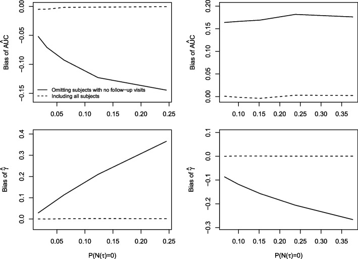 Figure 10
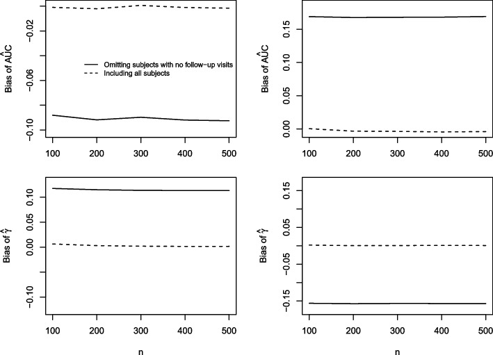 Figure 11
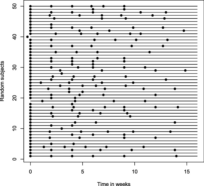 Figure 12
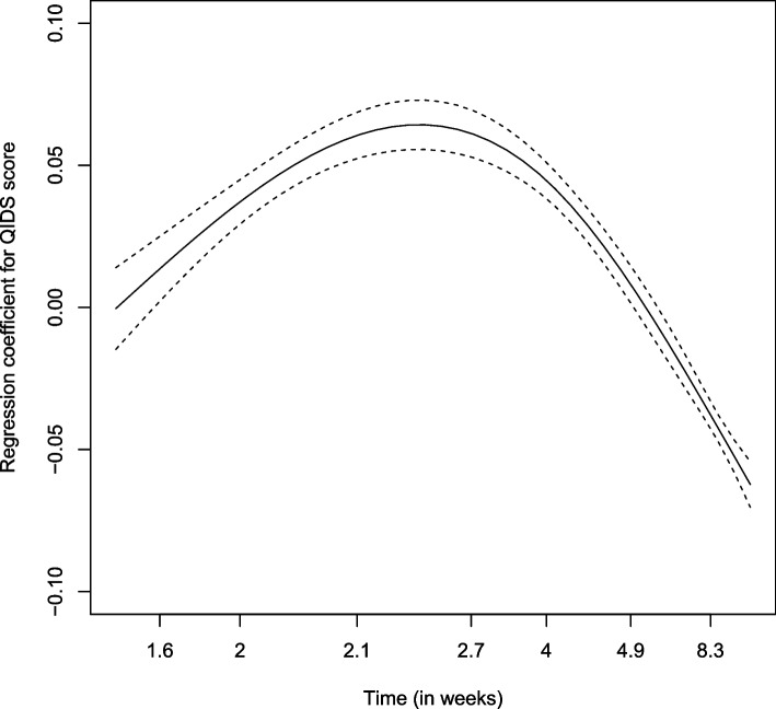 Figure 13
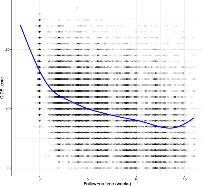 Figure 14
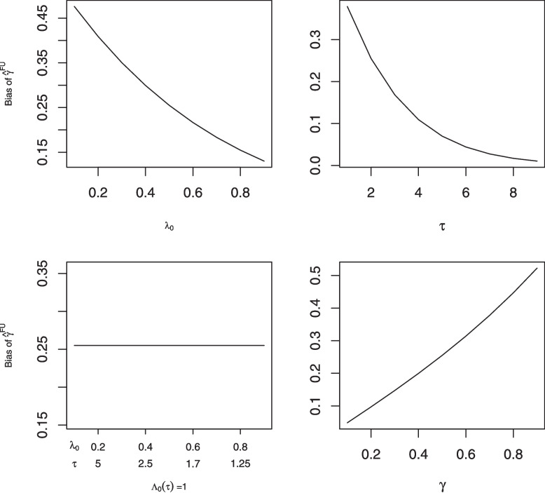 Figure 1
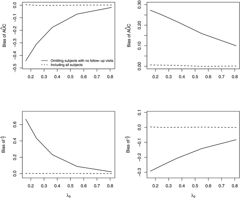 Figure 2
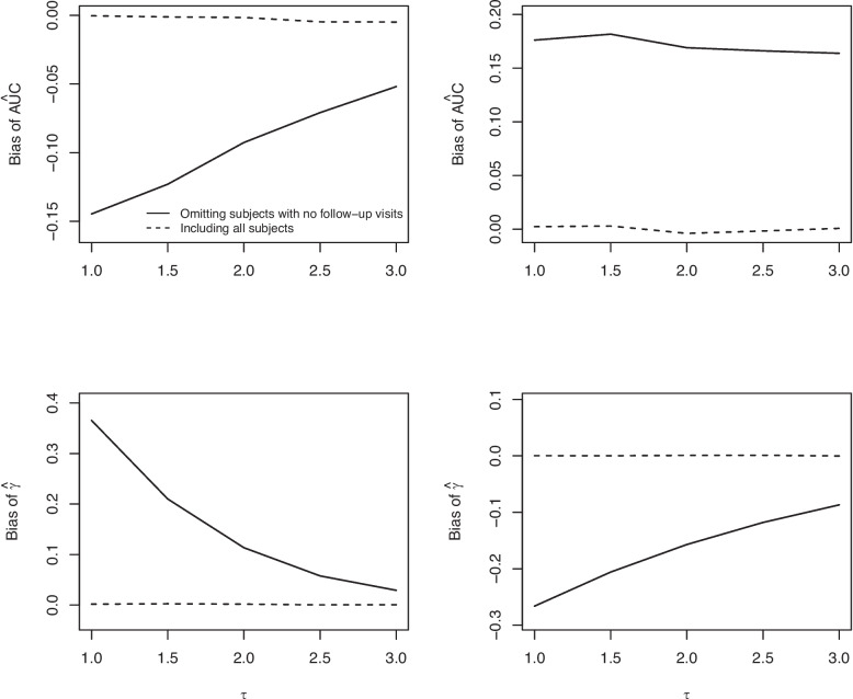 Figure 3
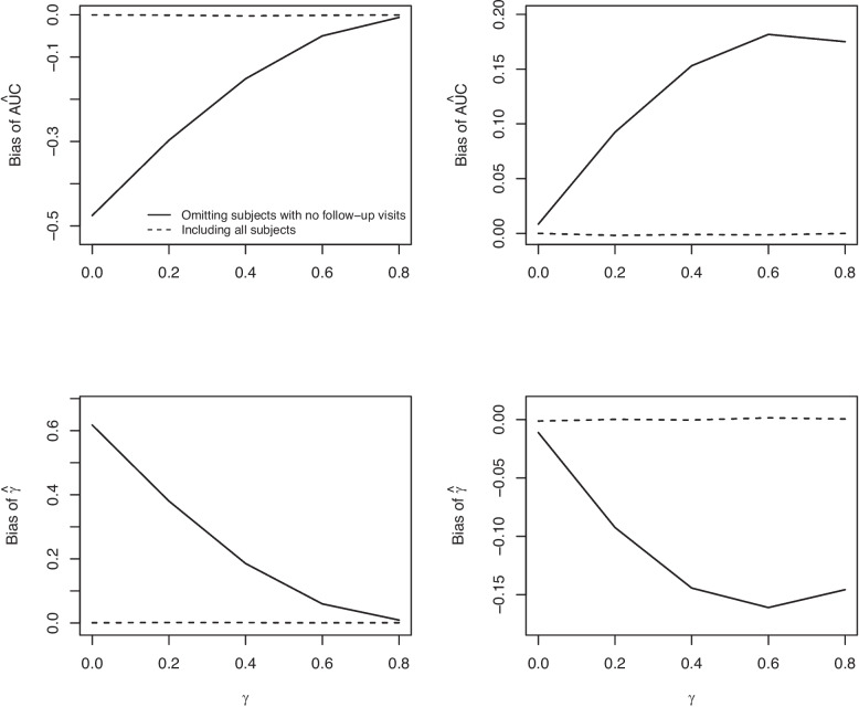 Figure 4
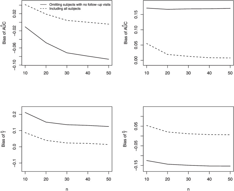 Figure 5
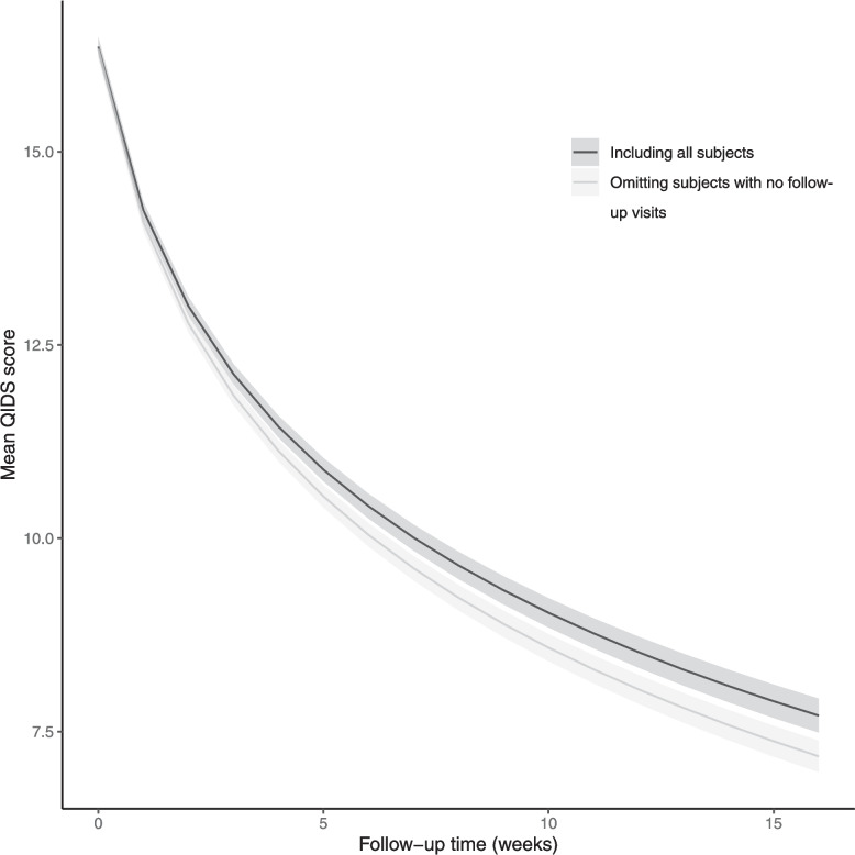 Figure 6
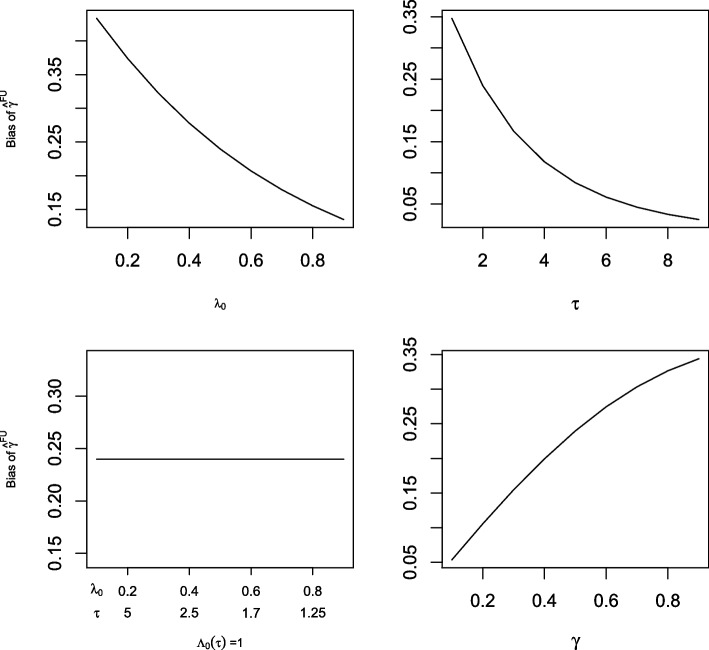 Figure 7
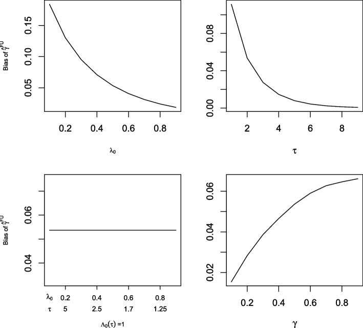 Figure 8
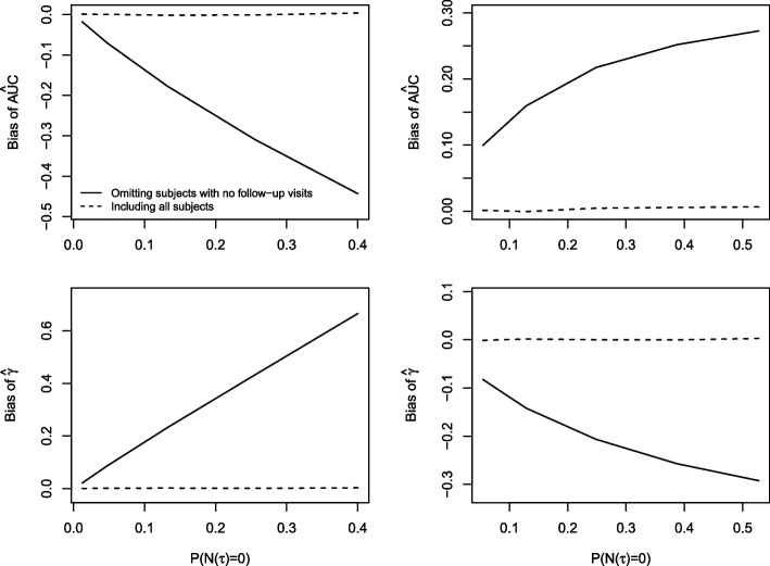 Figure 9
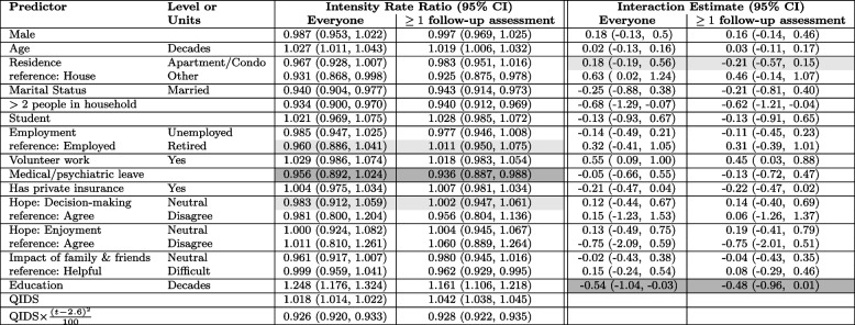 Figure 15
- —https://doi.org/10.13039/501100000038Natural Sciences and Engineering Research Council of Canada
Peer Reviews
No public reviews on file for this paper yet. If you reviewed it on a platform where reviews are public (OpenReview, ICLR, NeurIPS, ICML), you can paste yours below so the community can read it here.
Videos
No videos yet. Explain this paper in a talk, walkthrough, or lecture? Add one.
Taxonomy
TopicsMedication Adherence and Compliance · Health Systems, Economic Evaluations, Quality of Life · Chronic Disease Management Strategies
Background
Longitudinal data play a crucial role in studying prognosis and treatment effects over time. Outcomes are measured over time for each participant and studies typically aim to use these data to understand how outcomes evolve over time, or to assess whether specific treatments or patient characteristics lead to different outcome trajectories. In both observational and interventional studies, the times at which outcomes are assessed may be irregular, with the number of timing of assessments varying among subjects. This may occur, for example, if data is gathered through a chart review when all follow-up is part of usual care (see [1] for an example of a trial that used this design).
The timing of assessments is often related to study outcomes; for example, low weight gain in a neonate would trigger more frequent assessments. Dependence between outcomes and assessment frequency leads to standard methods of analysis such as Generalized Estimating Equations (GEEs) giving biased estimates of regression coefficients [2]. A range of methods have been proposed to handle irregular and informative assessment times, including inverse-intensity weighted generalized estimating equations (IIW-GEEs) [2] and semi-parametric joint models [3–6]; see [7] for a review. IIW-GEEs yield consistent inferences when the assessment time and outcome processes are conditionally independent given previously observed data, while semi-parametric joint models are appropriate when the assessment time and outcome processes are conditionally independent given random effects. In this paper we focus on IIW-GEEs as they are the most widely used [8], and unlike semi-parametric joint models can handle the common phenomenon of assessment times depending on a time-varying covariate.
A consequence of irregular assessment times is that there may be some patients with no follow-up at all. These patients are often excluded from analyses. For example, a review of prognosis studies in systemic lupus erythematosus found that 14% of studies used availability of the outcome as an inclusion criterion [9], and a review of longitudinal studies in older adults found that 75% of studies had exclusions due to lack of follow-up data [10].
Moreover, exclusion of patients with no follow-up may be unintentional and occurs through implicit inclusion criteria; this can happen when taking a subsample of an existing cohort or when creating a new cohort. For example, in studying the relationship between air quality and outoor play, Pullenayegum et al. [11, 12] used an inception cohort of children recruited through primary care clinics [13] and took a subsample of all measurements of outdoor play taken between the ages of 2 and 10 years. Consequently children who were enrolled in the original cohort but did not visit their doctor between the ages of 2 and the earlier of 10 years or the year data was cut were excluded from the dataset. A similar phenomenon can occur when creating a de novo cohort. For example, in studying the effect of statins on fasting glucose, Hadar et al. created their cohort by extracting fasting glucose measurements from an EHR database; thus only patients with a fasting glucose measurement were included in the dataset [14].
If the timing of assessments is unrelated to outcomes, these exclusions do not induce any selection bias. However, when the timing of assessments is related to outcomes, exclusion of patients with no follow-up raises concerns over bias because the assessment times are themselves informative about the outcome. While IIW-GEEs provide unbiased inferences when outcomes and assessment times are conditionally independent given previously observed data, this assumes that all patients are included in the analysis. The purpose of this paper is to examine whether exclusion of patients with no follow-up assessments causes bias in IIW-GEE estimates of regression coefficients. In the Theoretical results section we show theoretically that exclusion of patients with no follow-up will lead to bias in IIW-GEE estimates of regression coefficients. In the Simulation section we use simulation to explore factors influencing the extent of the bias, and in the Example: the STARD study section we use the Sequenced Treatment Alternatives to Relieve Depression (STARD) study [15] to illustrate the impact in practice. We conclude with a Discussion section by considering the implications for researchers dealing with data subject to irregular assessment times.
Theoretical results
In this section we show that omitting subjects with no follow-up assessments results in biased estimates of the assessment process parameters and consequently biased IIW-GEE estimates of the regression coefficients for the mean outcome model.
Notation
Suppose \documentclass[12pt]{minimal} \usepackage{amsmath} \usepackage{wasysym} \usepackage{amsfonts} \usepackage{amssymb} \usepackage{amsbsy} \usepackage{mathrsfs} \usepackage{upgreek} \setlength{\oddsidemargin}{-69pt} \begin{document}$$Y_i(t)$$\end{document} is the outcome for patient i at time t, with \documentclass[12pt]{minimal} \usepackage{amsmath} \usepackage{wasysym} \usepackage{amsfonts} \usepackage{amssymb} \usepackage{amsbsy} \usepackage{mathrsfs} \usepackage{upgreek} \setlength{\oddsidemargin}{-69pt} \begin{document}$$t \in [0,\tau ]$$\end{document} , and that we wish to fit the marginal model
\documentclass[12pt]{minimal} \usepackage{amsmath} \usepackage{wasysym} \usepackage{amsfonts} \usepackage{amssymb} \usepackage{amsbsy} \usepackage{mathrsfs} \usepackage{upgreek} \setlength{\oddsidemargin}{-69pt} \begin{document}$$\begin{aligned} E(Y_i(t)\mid \textbf{X}_i(t)) = \textbf{X}_i(t)\varvec{\beta }_0 \end{aligned}$$\end{document}for a row vector of covariates \documentclass[12pt]{minimal} \usepackage{amsmath} \usepackage{wasysym} \usepackage{amsfonts} \usepackage{amssymb} \usepackage{amsbsy} \usepackage{mathrsfs} \usepackage{upgreek} \setlength{\oddsidemargin}{-69pt} \begin{document}$$\textbf{X}_i(t)$$\end{document} and corresponding regression coefficients \documentclass[12pt]{minimal} \usepackage{amsmath} \usepackage{wasysym} \usepackage{amsfonts} \usepackage{amssymb} \usepackage{amsbsy} \usepackage{mathrsfs} \usepackage{upgreek} \setlength{\oddsidemargin}{-69pt} \begin{document}$$\varvec{\beta }_0$$\end{document} . We do not observe \documentclass[12pt]{minimal} \usepackage{amsmath} \usepackage{wasysym} \usepackage{amsfonts} \usepackage{amssymb} \usepackage{amsbsy} \usepackage{mathrsfs} \usepackage{upgreek} \setlength{\oddsidemargin}{-69pt} \begin{document}$$Y_i(t)$$\end{document} at every time point \documentclass[12pt]{minimal} \usepackage{amsmath} \usepackage{wasysym} \usepackage{amsfonts} \usepackage{amssymb} \usepackage{amsbsy} \usepackage{mathrsfs} \usepackage{upgreek} \setlength{\oddsidemargin}{-69pt} \begin{document}$$t\in [0,\tau ]$$\end{document} , but rather only when the patient comes in for a assessment.
Let \documentclass[12pt]{minimal} \usepackage{amsmath} \usepackage{wasysym} \usepackage{amsfonts} \usepackage{amssymb} \usepackage{amsbsy} \usepackage{mathrsfs} \usepackage{upgreek} \setlength{\oddsidemargin}{-69pt} \begin{document}$$N_i(t)$$\end{document} denote the number of follow-up assessments for patient i by time t, and let \documentclass[12pt]{minimal} \usepackage{amsmath} \usepackage{wasysym} \usepackage{amsfonts} \usepackage{amssymb} \usepackage{amsbsy} \usepackage{mathrsfs} \usepackage{upgreek} \setlength{\oddsidemargin}{-69pt} \begin{document}$$\Delta N_i(t) = \lim _{\delta \downarrow 0} (N_i(t) - N_i(t-\delta ))$$\end{document} ; thus \documentclass[12pt]{minimal} \usepackage{amsmath} \usepackage{wasysym} \usepackage{amsfonts} \usepackage{amssymb} \usepackage{amsbsy} \usepackage{mathrsfs} \usepackage{upgreek} \setlength{\oddsidemargin}{-69pt} \begin{document}$$\Delta N_i(t)$$\end{document} is equal to 1 if patient i has a visit at time t and 0 otherwise, and we set \documentclass[12pt]{minimal} \usepackage{amsmath} \usepackage{wasysym} \usepackage{amsfonts} \usepackage{amssymb} \usepackage{amsbsy} \usepackage{mathrsfs} \usepackage{upgreek} \setlength{\oddsidemargin}{-69pt} \begin{document}$$N_i(0)=0$$\end{document} . Suppose there is a set of observed covariates \documentclass[12pt]{minimal} \usepackage{amsmath} \usepackage{wasysym} \usepackage{amsfonts} \usepackage{amssymb} \usepackage{amsbsy} \usepackage{mathrsfs} \usepackage{upgreek} \setlength{\oddsidemargin}{-69pt} \begin{document}$$\textbf{Z}_i(t)$$\end{document} such that the outcome at time t is conditionally independent of whether a visit occurs at time t given the covariates at time t, i.e. \documentclass[12pt]{minimal} \usepackage{amsmath} \usepackage{wasysym} \usepackage{amsfonts} \usepackage{amssymb} \usepackage{amsbsy} \usepackage{mathrsfs} \usepackage{upgreek} \setlength{\oddsidemargin}{-69pt} \begin{document}$$\Delta N_i(t) \perp \!\!\! \perp Y_i(t) \mid \textbf{Z}_i(t)$$\end{document} . The covariates \documentclass[12pt]{minimal} \usepackage{amsmath} \usepackage{wasysym} \usepackage{amsfonts} \usepackage{amssymb} \usepackage{amsbsy} \usepackage{mathrsfs} \usepackage{upgreek} \setlength{\oddsidemargin}{-69pt} \begin{document}$$\textbf{Z}_i(t)$$\end{document} may contain elements of \documentclass[12pt]{minimal} \usepackage{amsmath} \usepackage{wasysym} \usepackage{amsfonts} \usepackage{amssymb} \usepackage{amsbsy} \usepackage{mathrsfs} \usepackage{upgreek} \setlength{\oddsidemargin}{-69pt} \begin{document}$$\textbf{X}_i(t)$$\end{document} and past observed values of \documentclass[12pt]{minimal} \usepackage{amsmath} \usepackage{wasysym} \usepackage{amsfonts} \usepackage{amssymb} \usepackage{amsbsy} \usepackage{mathrsfs} \usepackage{upgreek} \setlength{\oddsidemargin}{-69pt} \begin{document}$$Y_i(t)$$\end{document} , and may also contain auxiliary covariates not included in the outcome mean model. We assume that the assessment process intensity at time t conditional on \documentclass[12pt]{minimal} \usepackage{amsmath} \usepackage{wasysym} \usepackage{amsfonts} \usepackage{amssymb} \usepackage{amsbsy} \usepackage{mathrsfs} \usepackage{upgreek} \setlength{\oddsidemargin}{-69pt} \begin{document}$$\textbf{Z}_i(t)$$\end{document} follows a proportional hazards model, that is
\documentclass[12pt]{minimal} \usepackage{amsmath} \usepackage{wasysym} \usepackage{amsfonts} \usepackage{amssymb} \usepackage{amsbsy} \usepackage{mathrsfs} \usepackage{upgreek} \setlength{\oddsidemargin}{-69pt} \begin{document}$$\begin{aligned} \lambda (t;\textbf{Z}_i(t),\varvec{\gamma }_0) = \lim _{\delta \downarrow 0} \frac{E(N_i(t) - N_i(t-\delta )\mid \textbf{Z}_i(t))}{\delta } = \lambda _0(t){\textrm{exp}}(\textbf{Z}_i(t)\varvec{\gamma }_0), \end{aligned}$$\end{document}where the log hazard ratios \documentclass[12pt]{minimal} \usepackage{amsmath} \usepackage{wasysym} \usepackage{amsfonts} \usepackage{amssymb} \usepackage{amsbsy} \usepackage{mathrsfs} \usepackage{upgreek} \setlength{\oddsidemargin}{-69pt} \begin{document}$$\varvec{\gamma }_0$$\end{document} and the baseline hazard \documentclass[12pt]{minimal} \usepackage{amsmath} \usepackage{wasysym} \usepackage{amsfonts} \usepackage{amssymb} \usepackage{amsbsy} \usepackage{mathrsfs} \usepackage{upgreek} \setlength{\oddsidemargin}{-69pt} \begin{document}$$\lambda _0$$\end{document} are unknown.
Inverse-intensity weighted GEEs
The usual GEE equations under working independence can be written as
\documentclass[12pt]{minimal} \usepackage{amsmath} \usepackage{wasysym} \usepackage{amsfonts} \usepackage{amssymb} \usepackage{amsbsy} \usepackage{mathrsfs} \usepackage{upgreek} \setlength{\oddsidemargin}{-69pt} \begin{document}$$\begin{aligned} \sum \limits _i\int _0^\tau \textbf{X}_i(t)^\prime (Y_i(t)-\textbf{X}_i(t)\varvec{\beta })dN_i(t)=0 \end{aligned}$$\end{document}These result in biased estimates of the outcome model regression coefficients \documentclass[12pt]{minimal} \usepackage{amsmath} \usepackage{wasysym} \usepackage{amsfonts} \usepackage{amssymb} \usepackage{amsbsy} \usepackage{mathrsfs} \usepackage{upgreek} \setlength{\oddsidemargin}{-69pt} \begin{document}$$\varvec{\beta }_0$$\end{document} if \documentclass[12pt]{minimal} \usepackage{amsmath} \usepackage{wasysym} \usepackage{amsfonts} \usepackage{amssymb} \usepackage{amsbsy} \usepackage{mathrsfs} \usepackage{upgreek} \setlength{\oddsidemargin}{-69pt} \begin{document}$$Y_i(t)$$\end{document} and \documentclass[12pt]{minimal} \usepackage{amsmath} \usepackage{wasysym} \usepackage{amsfonts} \usepackage{amssymb} \usepackage{amsbsy} \usepackage{mathrsfs} \usepackage{upgreek} \setlength{\oddsidemargin}{-69pt} \begin{document}$$dN_i(t)$$\end{document} are dependent given \documentclass[12pt]{minimal} \usepackage{amsmath} \usepackage{wasysym} \usepackage{amsfonts} \usepackage{amssymb} \usepackage{amsbsy} \usepackage{mathrsfs} \usepackage{upgreek} \setlength{\oddsidemargin}{-69pt} \begin{document}$$\textbf{X}_i(t)$$\end{document} because the expectation of the left-hand side is no longer zero [2]. However, consistent estimates of \documentclass[12pt]{minimal} \usepackage{amsmath} \usepackage{wasysym} \usepackage{amsfonts} \usepackage{amssymb} \usepackage{amsbsy} \usepackage{mathrsfs} \usepackage{upgreek} \setlength{\oddsidemargin}{-69pt} \begin{document}$$\varvec{\beta }_0$$\end{document} can be obtained by solving the inverse-intensity weighted GEEs [2, 16], i.e. by solving
\documentclass[12pt]{minimal} \usepackage{amsmath} \usepackage{wasysym} \usepackage{amsfonts} \usepackage{amssymb} \usepackage{amsbsy} \usepackage{mathrsfs} \usepackage{upgreek} \setlength{\oddsidemargin}{-69pt} \begin{document}$$\begin{aligned} U(\varvec{\beta };\varvec{\gamma }_0) = \sum \limits _i\int _0^\tau \textbf{X}_i(t)^\prime \frac{(Y_i(t)-\textbf{X}_i(t)\varvec{\beta })}{{\textrm{exp}}(\textbf{Z}_i(t)\varvec{\gamma }_0)}dN_i(t)=0 \end{aligned}$$\end{document}Lin et al. [2] show that the mean of \documentclass[12pt]{minimal} \usepackage{amsmath} \usepackage{wasysym} \usepackage{amsfonts} \usepackage{amssymb} \usepackage{amsbsy} \usepackage{mathrsfs} \usepackage{upgreek} \setlength{\oddsidemargin}{-69pt} \begin{document}$$U(\varvec{\beta };\varvec{\gamma }_0)$$\end{document} is zero, and that the solution \documentclass[12pt]{minimal} \usepackage{amsmath} \usepackage{wasysym} \usepackage{amsfonts} \usepackage{amssymb} \usepackage{amsbsy} \usepackage{mathrsfs} \usepackage{upgreek} \setlength{\oddsidemargin}{-69pt} \begin{document}$$\hat{\varvec{\beta }}$$\end{document} to \documentclass[12pt]{minimal} \usepackage{amsmath} \usepackage{wasysym} \usepackage{amsfonts} \usepackage{amssymb} \usepackage{amsbsy} \usepackage{mathrsfs} \usepackage{upgreek} \setlength{\oddsidemargin}{-69pt} \begin{document}$$U(\varvec{\beta };\hat{\varvec{\gamma }})=0$$\end{document} is consistent provided that \documentclass[12pt]{minimal} \usepackage{amsmath} \usepackage{wasysym} \usepackage{amsfonts} \usepackage{amssymb} \usepackage{amsbsy} \usepackage{mathrsfs} \usepackage{upgreek} \setlength{\oddsidemargin}{-69pt} \begin{document}$$n^{1/2}(\hat{\varvec{\gamma }}-\varvec{\gamma })$$\end{document} is o(1). Maximizing the Cox partial likelihood for \documentclass[12pt]{minimal} \usepackage{amsmath} \usepackage{wasysym} \usepackage{amsfonts} \usepackage{amssymb} \usepackage{amsbsy} \usepackage{mathrsfs} \usepackage{upgreek} \setlength{\oddsidemargin}{-69pt} \begin{document}$$\varvec{\gamma }$$\end{document} using the full dataset yields an \documentclass[12pt]{minimal} \usepackage{amsmath} \usepackage{wasysym} \usepackage{amsfonts} \usepackage{amssymb} \usepackage{amsbsy} \usepackage{mathrsfs} \usepackage{upgreek} \setlength{\oddsidemargin}{-69pt} \begin{document}$$o(n^{-1/2})$$\end{document} -consistent estimate provided that the intensity model is correctly specified [17].
Bias due to omission of subjects with no follow-up assessments
We now consider the impact of excluding patients with no follow-up assessments. Let \documentclass[12pt]{minimal} \usepackage{amsmath} \usepackage{wasysym} \usepackage{amsfonts} \usepackage{amssymb} \usepackage{amsbsy} \usepackage{mathrsfs} \usepackage{upgreek} \setlength{\oddsidemargin}{-69pt} \begin{document}$$\varvec{\hat{\beta }}^{EV}$$\end{document} and \documentclass[12pt]{minimal} \usepackage{amsmath} \usepackage{wasysym} \usepackage{amsfonts} \usepackage{amssymb} \usepackage{amsbsy} \usepackage{mathrsfs} \usepackage{upgreek} \setlength{\oddsidemargin}{-69pt} \begin{document}$$\varvec{\hat{\gamma }}^{EV}$$\end{document} be the estimates of \documentclass[12pt]{minimal} \usepackage{amsmath} \usepackage{wasysym} \usepackage{amsfonts} \usepackage{amssymb} \usepackage{amsbsy} \usepackage{mathrsfs} \usepackage{upgreek} \setlength{\oddsidemargin}{-69pt} \begin{document}$$\varvec{\beta }$$\end{document} and \documentclass[12pt]{minimal} \usepackage{amsmath} \usepackage{wasysym} \usepackage{amsfonts} \usepackage{amssymb} \usepackage{amsbsy} \usepackage{mathrsfs} \usepackage{upgreek} \setlength{\oddsidemargin}{-69pt} \begin{document}$$\varvec{\gamma }$$\end{document} on using everyone, and \documentclass[12pt]{minimal} \usepackage{amsmath} \usepackage{wasysym} \usepackage{amsfonts} \usepackage{amssymb} \usepackage{amsbsy} \usepackage{mathrsfs} \usepackage{upgreek} \setlength{\oddsidemargin}{-69pt} \begin{document}$$\varvec{\hat{\beta }}^{FU}$$\end{document} and \documentclass[12pt]{minimal} \usepackage{amsmath} \usepackage{wasysym} \usepackage{amsfonts} \usepackage{amssymb} \usepackage{amsbsy} \usepackage{mathrsfs} \usepackage{upgreek} \setlength{\oddsidemargin}{-69pt} \begin{document}$$\varvec{\hat{\gamma }}^{FU}$$\end{document} be the estimates of \documentclass[12pt]{minimal} \usepackage{amsmath} \usepackage{wasysym} \usepackage{amsfonts} \usepackage{amssymb} \usepackage{amsbsy} \usepackage{mathrsfs} \usepackage{upgreek} \setlength{\oddsidemargin}{-69pt} \begin{document}$$\varvec{\beta }$$\end{document} and \documentclass[12pt]{minimal} \usepackage{amsmath} \usepackage{wasysym} \usepackage{amsfonts} \usepackage{amssymb} \usepackage{amsbsy} \usepackage{mathrsfs} \usepackage{upgreek} \setlength{\oddsidemargin}{-69pt} \begin{document}$$\varvec{\gamma }$$\end{document} on omitting patients with no follow-up assessments. For any given \documentclass[12pt]{minimal} \usepackage{amsmath} \usepackage{wasysym} \usepackage{amsfonts} \usepackage{amssymb} \usepackage{amsbsy} \usepackage{mathrsfs} \usepackage{upgreek} \setlength{\oddsidemargin}{-69pt} \begin{document}$$\varvec{\gamma }$$\end{document} , \documentclass[12pt]{minimal} \usepackage{amsmath} \usepackage{wasysym} \usepackage{amsfonts} \usepackage{amssymb} \usepackage{amsbsy} \usepackage{mathrsfs} \usepackage{upgreek} \setlength{\oddsidemargin}{-69pt} \begin{document}$$U(\varvec{\beta };\varvec{\gamma })$$\end{document} remains unchanged on omitting subjects with no follow-up assessments:
\documentclass[12pt]{minimal} \usepackage{amsmath} \usepackage{wasysym} \usepackage{amsfonts} \usepackage{amssymb} \usepackage{amsbsy} \usepackage{mathrsfs} \usepackage{upgreek} \setlength{\oddsidemargin}{-69pt} \begin{document}$$\begin{aligned} U(\varvec{\beta };\varvec{\gamma })= & \sum \limits _{i}\int _0^\tau \textbf{X}_i(t)^\prime (Y_i(t)-\textbf{X}_i(t)\varvec{\beta }){\textrm{exp}}(-\textbf{Z}_i(t)\varvec{\gamma })dN_i(t) \\= & \sum \limits _{i:N_i(\tau )>0}\int _0^\tau \textbf{X}_i(t)^\prime (Y_i(t)-\textbf{X}_i(t)\varvec{\beta }){\textrm{exp}}(-\textbf{Z}_i(t)\varvec{\gamma })dN_i(t) \end{aligned}$$\end{document}As excluding subjects with no follow-up assessments has no impact on the pseudo-score function \documentclass[12pt]{minimal} \usepackage{amsmath} \usepackage{wasysym} \usepackage{amsfonts} \usepackage{amssymb} \usepackage{amsbsy} \usepackage{mathrsfs} \usepackage{upgreek} \setlength{\oddsidemargin}{-69pt} \begin{document}$$U(\varvec{\beta };\varvec{\gamma })$$\end{document} , any bias in \documentclass[12pt]{minimal} \usepackage{amsmath} \usepackage{wasysym} \usepackage{amsfonts} \usepackage{amssymb} \usepackage{amsbsy} \usepackage{mathrsfs} \usepackage{upgreek} \setlength{\oddsidemargin}{-69pt} \begin{document}$$\varvec{\hat{\beta }}^{FU}$$\end{document} induced by omitting patients with no follow-up assessments will occur due to bias in \documentclass[12pt]{minimal} \usepackage{amsmath} \usepackage{wasysym} \usepackage{amsfonts} \usepackage{amssymb} \usepackage{amsbsy} \usepackage{mathrsfs} \usepackage{upgreek} \setlength{\oddsidemargin}{-69pt} \begin{document}$$\varvec{\hat{\gamma }}^{FU}$$\end{document} . In the special case where the assessment intensity covariates \documentclass[12pt]{minimal} \usepackage{amsmath} \usepackage{wasysym} \usepackage{amsfonts} \usepackage{amssymb} \usepackage{amsbsy} \usepackage{mathrsfs} \usepackage{upgreek} \setlength{\oddsidemargin}{-69pt} \begin{document}$$\textbf{Z}_i$$\end{document} and the baseline hazard \documentclass[12pt]{minimal} \usepackage{amsmath} \usepackage{wasysym} \usepackage{amsfonts} \usepackage{amssymb} \usepackage{amsbsy} \usepackage{mathrsfs} \usepackage{upgreek} \setlength{\oddsidemargin}{-69pt} \begin{document}$$\lambda _0$$\end{document} are time-independent, a Taylor expansion of \documentclass[12pt]{minimal} \usepackage{amsmath} \usepackage{wasysym} \usepackage{amsfonts} \usepackage{amssymb} \usepackage{amsbsy} \usepackage{mathrsfs} \usepackage{upgreek} \setlength{\oddsidemargin}{-69pt} \begin{document}$$U(\varvec{\beta };\varvec{\hat{\gamma }}^{FU})$$\end{document} about \documentclass[12pt]{minimal} \usepackage{amsmath} \usepackage{wasysym} \usepackage{amsfonts} \usepackage{amssymb} \usepackage{amsbsy} \usepackage{mathrsfs} \usepackage{upgreek} \setlength{\oddsidemargin}{-69pt} \begin{document}$$\varvec{\gamma }_0$$\end{document} yields, to first order,
\documentclass[12pt]{minimal} \usepackage{amsmath} \usepackage{wasysym} \usepackage{amsfonts} \usepackage{amssymb} \usepackage{amsbsy} \usepackage{mathrsfs} \usepackage{upgreek} \setlength{\oddsidemargin}{-69pt} \begin{document}$$\begin{aligned} & E(\varvec{\hat{\beta }}^{FU}-\varvec{\beta }_0) =-\left( \int _0^\tau E \left( \textbf{X}_i(t)^\prime \textbf{X}_i(t) \right) dt\right) ^{-1} \\ & E\left( \int _0^\tau E\left( \textbf{X}_i(t)^\prime (Y_i(t)-\textbf{X}_i(t)\varvec{\beta }_0)\mid \textbf{Z}_i\right) dt\textbf{Z}_iE(\hat{\gamma }^{FU}-\varvec{\gamma }_0\mid \textbf{Z}_i)\right) \end{aligned}$$\end{document}(see Appendix A for a general derivation). Thus if \documentclass[12pt]{minimal} \usepackage{amsmath} \usepackage{wasysym} \usepackage{amsfonts} \usepackage{amssymb} \usepackage{amsbsy} \usepackage{mathrsfs} \usepackage{upgreek} \setlength{\oddsidemargin}{-69pt} \begin{document}$$\varvec{\hat{\gamma }}^{FU}$$\end{document} is biased, \documentclass[12pt]{minimal} \usepackage{amsmath} \usepackage{wasysym} \usepackage{amsfonts} \usepackage{amssymb} \usepackage{amsbsy} \usepackage{mathrsfs} \usepackage{upgreek} \setlength{\oddsidemargin}{-69pt} \begin{document}$$\varvec{\hat{\beta }}^{FU}$$\end{document} will also be biased.
Bias in the inverse intensity weights
In Appendix A we give a general expression for the bias in \documentclass[12pt]{minimal} \usepackage{amsmath} \usepackage{wasysym} \usepackage{amsfonts} \usepackage{amssymb} \usepackage{amsbsy} \usepackage{mathrsfs} \usepackage{upgreek} \setlength{\oddsidemargin}{-69pt} \begin{document}$$\varvec{\hat{\gamma }}^{FU}$$\end{document} . In the special case where the intensity covariates \documentclass[12pt]{minimal} \usepackage{amsmath} \usepackage{wasysym} \usepackage{amsfonts} \usepackage{amssymb} \usepackage{amsbsy} \usepackage{mathrsfs} \usepackage{upgreek} \setlength{\oddsidemargin}{-69pt} \begin{document}$$\textbf{Z}_i$$\end{document} and the baseline hazard \documentclass[12pt]{minimal} \usepackage{amsmath} \usepackage{wasysym} \usepackage{amsfonts} \usepackage{amssymb} \usepackage{amsbsy} \usepackage{mathrsfs} \usepackage{upgreek} \setlength{\oddsidemargin}{-69pt} \begin{document}$$\lambda _0$$\end{document} are time-invariant, this expression simplifies to
\documentclass[12pt]{minimal} \usepackage{amsmath} \usepackage{wasysym} \usepackage{amsfonts} \usepackage{amssymb} \usepackage{amsbsy} \usepackage{mathrsfs} \usepackage{upgreek} \setlength{\oddsidemargin}{-69pt} \begin{document}$$\begin{aligned} -\left( \left( \frac{s_1^*(\varvec{\gamma }_0)}{s_0^*(\varvec{\gamma }_0)}\right) ^2-\frac{s_2^*(\varvec{\gamma }_0)}{s_0^*(\varvec{\gamma }_0)}\right) ^{-1} \left( \frac{s_1^*(\varvec{\gamma }_0)}{s_0^*(\varvec{\gamma }_0)}- \frac{s_1(\varvec{\gamma }_0)}{s_0(\varvec{\gamma }_0)}\right) \end{aligned}$$\end{document}where
\documentclass[12pt]{minimal} \usepackage{amsmath} \usepackage{wasysym} \usepackage{amsfonts} \usepackage{amssymb} \usepackage{amsbsy} \usepackage{mathrsfs} \usepackage{upgreek} \setlength{\oddsidemargin}{-69pt} \begin{document}$$\begin{aligned} \begin{array}{ll} s_0(\varvec{\gamma }_0)=E({\textrm{exp}}(\varvec{\gamma }_0^{\prime } \textbf{Z}_i)) & s_0^*(\varvec{\gamma }_0)=E({\textrm{exp}}(\varvec{\gamma }_0^{\prime } \textbf{Z}_i)\mid N_i(\tau )>0) \\ \textbf{s}_1(\varvec{\gamma }_0)=E(\textbf{Z}_i{\textrm{exp}}(\varvec{\gamma }_0^{\prime } \textbf{Z}_i)) & \textbf{s}_1^*(\varvec{\gamma }_0)=E(\textbf{Z}_i{\textrm{exp}}(\varvec{\gamma }_0^{\prime } Z_j)\mid N_i(\tau )>0)\\ \textbf{s}_2(\varvec{\gamma }_0)=E(\textbf{Z}_i\textbf{Z}_i^\prime {\textrm{exp}}(\varvec{\gamma }_0^{\prime } \textbf{Z}_i)) & \textbf{s}_2^*(\varvec{\gamma }_0)=E(\textbf{Z}_i\textbf{Z}_i^\prime {\textrm{exp}}(\varvec{\gamma }_0^{\prime } \textbf{Z}_i)\mid N_i(\tau )>0)\\ \end{array} \end{aligned}$$\end{document}Since both \documentclass[12pt]{minimal} \usepackage{amsmath} \usepackage{wasysym} \usepackage{amsfonts} \usepackage{amssymb} \usepackage{amsbsy} \usepackage{mathrsfs} \usepackage{upgreek} \setlength{\oddsidemargin}{-69pt} \begin{document}$$\textbf{Z}_i$$\end{document} and \documentclass[12pt]{minimal} \usepackage{amsmath} \usepackage{wasysym} \usepackage{amsfonts} \usepackage{amssymb} \usepackage{amsbsy} \usepackage{mathrsfs} \usepackage{upgreek} \setlength{\oddsidemargin}{-69pt} \begin{document}$$\lambda _0$$\end{document} are time-invariant, \documentclass[12pt]{minimal} \usepackage{amsmath} \usepackage{wasysym} \usepackage{amsfonts} \usepackage{amssymb} \usepackage{amsbsy} \usepackage{mathrsfs} \usepackage{upgreek} \setlength{\oddsidemargin}{-69pt} \begin{document}$$N_j(\tau )\mid \textbf{Z}_i\sim \text {Poisson}( \lambda _0{\textrm{exp}}(\varvec{\gamma }_0^\prime \textbf{Z}_i)\tau )$$\end{document} . It follows that if \documentclass[12pt]{minimal} \usepackage{amsmath} \usepackage{wasysym} \usepackage{amsfonts} \usepackage{amssymb} \usepackage{amsbsy} \usepackage{mathrsfs} \usepackage{upgreek} \setlength{\oddsidemargin}{-69pt} \begin{document}$$\varvec{\gamma }_0$$\end{document} is positive, when we omit patients with no follow-up assessments we will tend to see larger values of the covariates \documentclass[12pt]{minimal} \usepackage{amsmath} \usepackage{wasysym} \usepackage{amsfonts} \usepackage{amssymb} \usepackage{amsbsy} \usepackage{mathrsfs} \usepackage{upgreek} \setlength{\oddsidemargin}{-69pt} \begin{document}$$\textbf{Z}_i$$\end{document} , so that \documentclass[12pt]{minimal} \usepackage{amsmath} \usepackage{wasysym} \usepackage{amsfonts} \usepackage{amssymb} \usepackage{amsbsy} \usepackage{mathrsfs} \usepackage{upgreek} \setlength{\oddsidemargin}{-69pt} \begin{document}$$s_0^*>s_0$$\end{document} and \documentclass[12pt]{minimal} \usepackage{amsmath} \usepackage{wasysym} \usepackage{amsfonts} \usepackage{amssymb} \usepackage{amsbsy} \usepackage{mathrsfs} \usepackage{upgreek} \setlength{\oddsidemargin}{-69pt} \begin{document}$$\textbf{s}_1^*>\textbf{s}_1$$\end{document} . In fact it is possible to evaluate the conditional expectations in the expressions for \documentclass[12pt]{minimal} \usepackage{amsmath} \usepackage{wasysym} \usepackage{amsfonts} \usepackage{amssymb} \usepackage{amsbsy} \usepackage{mathrsfs} \usepackage{upgreek} \setlength{\oddsidemargin}{-69pt} \begin{document}$$s_0^*$$\end{document} and \documentclass[12pt]{minimal} \usepackage{amsmath} \usepackage{wasysym} \usepackage{amsfonts} \usepackage{amssymb} \usepackage{amsbsy} \usepackage{mathrsfs} \usepackage{upgreek} \setlength{\oddsidemargin}{-69pt} \begin{document}$$s_1^*$$\end{document} given the distribution of \documentclass[12pt]{minimal} \usepackage{amsmath} \usepackage{wasysym} \usepackage{amsfonts} \usepackage{amssymb} \usepackage{amsbsy} \usepackage{mathrsfs} \usepackage{upgreek} \setlength{\oddsidemargin}{-69pt} \begin{document}$$\textbf{Z}$$\end{document} analytically. Here we consider \documentclass[12pt]{minimal} \usepackage{amsmath} \usepackage{wasysym} \usepackage{amsfonts} \usepackage{amssymb} \usepackage{amsbsy} \usepackage{mathrsfs} \usepackage{upgreek} \setlength{\oddsidemargin}{-69pt} \begin{document}$$Z_i\sim$$\end{document} Bernoulli(0.5), and provide results for \documentclass[12pt]{minimal} \usepackage{amsmath} \usepackage{wasysym} \usepackage{amsfonts} \usepackage{amssymb} \usepackage{amsbsy} \usepackage{mathrsfs} \usepackage{upgreek} \setlength{\oddsidemargin}{-69pt} \begin{document}$$Z_i\sim$$\end{document} Normal(0,1) and \documentclass[12pt]{minimal} \usepackage{amsmath} \usepackage{wasysym} \usepackage{amsfonts} \usepackage{amssymb} \usepackage{amsbsy} \usepackage{mathrsfs} \usepackage{upgreek} \setlength{\oddsidemargin}{-69pt} \begin{document}$$Z_i\sim$$\end{document} Gamma(1,1) in Appendix A.
As can be seen from Fig. 1, the magnitude of the bias of \documentclass[12pt]{minimal} \usepackage{amsmath} \usepackage{wasysym} \usepackage{amsfonts} \usepackage{amssymb} \usepackage{amsbsy} \usepackage{mathrsfs} \usepackage{upgreek} \setlength{\oddsidemargin}{-69pt} \begin{document}$$\hat{\gamma }^{FU}$$\end{document} decreases as either the baseline hazard \documentclass[12pt]{minimal} \usepackage{amsmath} \usepackage{wasysym} \usepackage{amsfonts} \usepackage{amssymb} \usepackage{amsbsy} \usepackage{mathrsfs} \usepackage{upgreek} \setlength{\oddsidemargin}{-69pt} \begin{document}$$\lambda _0$$\end{document} or the follow-up time \documentclass[12pt]{minimal} \usepackage{amsmath} \usepackage{wasysym} \usepackage{amsfonts} \usepackage{amssymb} \usepackage{amsbsy} \usepackage{mathrsfs} \usepackage{upgreek} \setlength{\oddsidemargin}{-69pt} \begin{document}$$\tau$$\end{document} increases. If \documentclass[12pt]{minimal} \usepackage{amsmath} \usepackage{wasysym} \usepackage{amsfonts} \usepackage{amssymb} \usepackage{amsbsy} \usepackage{mathrsfs} \usepackage{upgreek} \setlength{\oddsidemargin}{-69pt} \begin{document}$$\lambda _0$$\end{document} and \documentclass[12pt]{minimal} \usepackage{amsmath} \usepackage{wasysym} \usepackage{amsfonts} \usepackage{amssymb} \usepackage{amsbsy} \usepackage{mathrsfs} \usepackage{upgreek} \setlength{\oddsidemargin}{-69pt} \begin{document}$$\tau$$\end{document} are changed while keeping \documentclass[12pt]{minimal} \usepackage{amsmath} \usepackage{wasysym} \usepackage{amsfonts} \usepackage{amssymb} \usepackage{amsbsy} \usepackage{mathrsfs} \usepackage{upgreek} \setlength{\oddsidemargin}{-69pt} \begin{document}$$\Lambda _0(\tau )=\lambda _0\tau$$\end{document} constant, the bias of \documentclass[12pt]{minimal} \usepackage{amsmath} \usepackage{wasysym} \usepackage{amsfonts} \usepackage{amssymb} \usepackage{amsbsy} \usepackage{mathrsfs} \usepackage{upgreek} \setlength{\oddsidemargin}{-69pt} \begin{document}$$\hat{\gamma }^{FU}$$\end{document} remains unchanged. This makes sense, since the probability of no follow-up assessments is \documentclass[12pt]{minimal} \usepackage{amsmath} \usepackage{wasysym} \usepackage{amsfonts} \usepackage{amssymb} \usepackage{amsbsy} \usepackage{mathrsfs} \usepackage{upgreek} \setlength{\oddsidemargin}{-69pt} \begin{document}$${\textrm{exp}}(-\lambda _0\tau {\textrm{exp}}(\gamma _0^\prime Z_i))$$\end{document} , which decreases as either \documentclass[12pt]{minimal} \usepackage{amsmath} \usepackage{wasysym} \usepackage{amsfonts} \usepackage{amssymb} \usepackage{amsbsy} \usepackage{mathrsfs} \usepackage{upgreek} \setlength{\oddsidemargin}{-69pt} \begin{document}$$\lambda _0$$\end{document} or \documentclass[12pt]{minimal} \usepackage{amsmath} \usepackage{wasysym} \usepackage{amsfonts} \usepackage{amssymb} \usepackage{amsbsy} \usepackage{mathrsfs} \usepackage{upgreek} \setlength{\oddsidemargin}{-69pt} \begin{document}$$\tau$$\end{document} increases. Moreover, \documentclass[12pt]{minimal} \usepackage{amsmath} \usepackage{wasysym} \usepackage{amsfonts} \usepackage{amssymb} \usepackage{amsbsy} \usepackage{mathrsfs} \usepackage{upgreek} \setlength{\oddsidemargin}{-69pt} \begin{document}$$\lambda _0$$\end{document} and \documentclass[12pt]{minimal} \usepackage{amsmath} \usepackage{wasysym} \usepackage{amsfonts} \usepackage{amssymb} \usepackage{amsbsy} \usepackage{mathrsfs} \usepackage{upgreek} \setlength{\oddsidemargin}{-69pt} \begin{document}$$\tau$$\end{document} affect the probability of a subject having no follow-up assessments only through their product.
Increasing \documentclass[12pt]{minimal} \usepackage{amsmath} \usepackage{wasysym} \usepackage{amsfonts} \usepackage{amssymb} \usepackage{amsbsy} \usepackage{mathrsfs} \usepackage{upgreek} \setlength{\oddsidemargin}{-69pt} \begin{document}$$\varvec{\gamma }_0$$\end{document} while decreasing \documentclass[12pt]{minimal} \usepackage{amsmath} \usepackage{wasysym} \usepackage{amsfonts} \usepackage{amssymb} \usepackage{amsbsy} \usepackage{mathrsfs} \usepackage{upgreek} \setlength{\oddsidemargin}{-69pt} \begin{document}$$\lambda _0$$\end{document} to keep the mean number of assessments constant leads to increased bias of \documentclass[12pt]{minimal} \usepackage{amsmath} \usepackage{wasysym} \usepackage{amsfonts} \usepackage{amssymb} \usepackage{amsbsy} \usepackage{mathrsfs} \usepackage{upgreek} \setlength{\oddsidemargin}{-69pt} \begin{document}$$\hat{\gamma }^{FU}$$\end{document} (Fig. 1, bottom right panel). Intuitively this makes sense because when \documentclass[12pt]{minimal} \usepackage{amsmath} \usepackage{wasysym} \usepackage{amsfonts} \usepackage{amssymb} \usepackage{amsbsy} \usepackage{mathrsfs} \usepackage{upgreek} \setlength{\oddsidemargin}{-69pt} \begin{document}$$\varvec{\gamma }_0$$\end{document} is zero the assessment process is independent of \documentclass[12pt]{minimal} \usepackage{amsmath} \usepackage{wasysym} \usepackage{amsfonts} \usepackage{amssymb} \usepackage{amsbsy} \usepackage{mathrsfs} \usepackage{upgreek} \setlength{\oddsidemargin}{-69pt} \begin{document}$$\textbf{Z}_i$$\end{document} and we would not expect omission of subjects with no follow-up assessments to lead to bias.
Similar results hold for \documentclass[12pt]{minimal} \usepackage{amsmath} \usepackage{wasysym} \usepackage{amsfonts} \usepackage{amssymb} \usepackage{amsbsy} \usepackage{mathrsfs} \usepackage{upgreek} \setlength{\oddsidemargin}{-69pt} \begin{document}$$Z_i\sim$$\end{document} Normal(0,1) and \documentclass[12pt]{minimal} \usepackage{amsmath} \usepackage{wasysym} \usepackage{amsfonts} \usepackage{amssymb} \usepackage{amsbsy} \usepackage{mathrsfs} \usepackage{upgreek} \setlength{\oddsidemargin}{-69pt} \begin{document}$$Z_i\sim$$\end{document} Gamma(1,1) (see Appendix A).Fig. 1. Bias in the regression coefficient \documentclass[12pt]{minimal} \usepackage{amsmath} \usepackage{wasysym} \usepackage{amsfonts} \usepackage{amssymb} \usepackage{amsbsy} \usepackage{mathrsfs} \usepackage{upgreek} \setlength{\oddsidemargin}{-69pt} \begin{document}$$\hat{\gamma }$$\end{document} in the assessment intensity model for a single time-invariant covariate \documentclass[12pt]{minimal} \usepackage{amsmath} \usepackage{wasysym} \usepackage{amsfonts} \usepackage{amssymb} \usepackage{amsbsy} \usepackage{mathrsfs} \usepackage{upgreek} \setlength{\oddsidemargin}{-69pt} \begin{document}$$Z_j \sim$$\end{document} Bernoulli(0.5) as: the time-invariant assessment intensity \documentclass[12pt]{minimal} \usepackage{amsmath} \usepackage{wasysym} \usepackage{amsfonts} \usepackage{amssymb} \usepackage{amsbsy} \usepackage{mathrsfs} \usepackage{upgreek} \setlength{\oddsidemargin}{-69pt} \begin{document}$$\lambda _0$$\end{document} is varied (top left); the total follow-up time \documentclass[12pt]{minimal} \usepackage{amsmath} \usepackage{wasysym} \usepackage{amsfonts} \usepackage{amssymb} \usepackage{amsbsy} \usepackage{mathrsfs} \usepackage{upgreek} \setlength{\oddsidemargin}{-69pt} \begin{document}$$\tau$$\end{document} is varied (top right); \documentclass[12pt]{minimal} \usepackage{amsmath} \usepackage{wasysym} \usepackage{amsfonts} \usepackage{amssymb} \usepackage{amsbsy} \usepackage{mathrsfs} \usepackage{upgreek} \setlength{\oddsidemargin}{-69pt} \begin{document}$$\lambda _0$$\end{document} and \documentclass[12pt]{minimal} \usepackage{amsmath} \usepackage{wasysym} \usepackage{amsfonts} \usepackage{amssymb} \usepackage{amsbsy} \usepackage{mathrsfs} \usepackage{upgreek} \setlength{\oddsidemargin}{-69pt} \begin{document}$$\tau$$\end{document} are varied while holding \documentclass[12pt]{minimal} \usepackage{amsmath} \usepackage{wasysym} \usepackage{amsfonts} \usepackage{amssymb} \usepackage{amsbsy} \usepackage{mathrsfs} \usepackage{upgreek} \setlength{\oddsidemargin}{-69pt} \begin{document}$$\Lambda _0(\tau )(=\lambda _0 \times \tau )$$\end{document} fixed (bottom left); \documentclass[12pt]{minimal} \usepackage{amsmath} \usepackage{wasysym} \usepackage{amsfonts} \usepackage{amssymb} \usepackage{amsbsy} \usepackage{mathrsfs} \usepackage{upgreek} \setlength{\oddsidemargin}{-69pt} \begin{document}$$\gamma$$\end{document} is varied while decreasing \documentclass[12pt]{minimal} \usepackage{amsmath} \usepackage{wasysym} \usepackage{amsfonts} \usepackage{amssymb} \usepackage{amsbsy} \usepackage{mathrsfs} \usepackage{upgreek} \setlength{\oddsidemargin}{-69pt} \begin{document}$$\lambda _0$$\end{document} to hold the expected number of assessments constant (bottom right)
Simulation
Simulation set-Up
While closed-form expressions for the bias in \documentclass[12pt]{minimal} \usepackage{amsmath} \usepackage{wasysym} \usepackage{amsfonts} \usepackage{amssymb} \usepackage{amsbsy} \usepackage{mathrsfs} \usepackage{upgreek} \setlength{\oddsidemargin}{-69pt} \begin{document}$$\varvec{\hat{\beta }}^{FU}$$\end{document} are available when the intensity model covariates \documentclass[12pt]{minimal} \usepackage{amsmath} \usepackage{wasysym} \usepackage{amsfonts} \usepackage{amssymb} \usepackage{amsbsy} \usepackage{mathrsfs} \usepackage{upgreek} \setlength{\oddsidemargin}{-69pt} \begin{document}$$\varvec{Z}$$\end{document} are time-invariant, this is not the case for time-varying \documentclass[12pt]{minimal} \usepackage{amsmath} \usepackage{wasysym} \usepackage{amsfonts} \usepackage{amssymb} \usepackage{amsbsy} \usepackage{mathrsfs} \usepackage{upgreek} \setlength{\oddsidemargin}{-69pt} \begin{document}$$\varvec{Z}$$\end{document} . We used a simulation study that aimed to examine the bias when omitting subjects with no follow-up assessments when \documentclass[12pt]{minimal} \usepackage{amsmath} \usepackage{wasysym} \usepackage{amsfonts} \usepackage{amssymb} \usepackage{amsbsy} \usepackage{mathrsfs} \usepackage{upgreek} \setlength{\oddsidemargin}{-69pt} \begin{document}$$\varvec{Z}$$\end{document} is time-varying. Specific hypotheses are outlined in Table 1.Table 1. Simulation parameters, hypotheses and results. Unless otherwise specified, \documentclass[12pt]{minimal} \usepackage{amsmath} \usepackage{wasysym} \usepackage{amsfonts} \usepackage{amssymb} \usepackage{amsbsy} \usepackage{mathrsfs} \usepackage{upgreek} \setlength{\oddsidemargin}{-69pt} \begin{document}$$\lambda _0=0.5$$\end{document} , \documentclass[12pt]{minimal} \usepackage{amsmath} \usepackage{wasysym} \usepackage{amsfonts} \usepackage{amssymb} \usepackage{amsbsy} \usepackage{mathrsfs} \usepackage{upgreek} \setlength{\oddsidemargin}{-69pt} \begin{document}$$\varvec{\gamma }_0=0.5$$\end{document} , \documentclass[12pt]{minimal} \usepackage{amsmath} \usepackage{wasysym} \usepackage{amsfonts} \usepackage{amssymb} \usepackage{amsbsy} \usepackage{mathrsfs} \usepackage{upgreek} \setlength{\oddsidemargin}{-69pt} \begin{document}$$n=500$$\end{document} , \documentclass[12pt]{minimal} \usepackage{amsmath} \usepackage{wasysym} \usepackage{amsfonts} \usepackage{amssymb} \usepackage{amsbsy} \usepackage{mathrsfs} \usepackage{upgreek} \setlength{\oddsidemargin}{-69pt} \begin{document}$$\tau =2$$\end{document} . We consider two data-generating mechanisms, one with \documentclass[12pt]{minimal} \usepackage{amsmath} \usepackage{wasysym} \usepackage{amsfonts} \usepackage{amssymb} \usepackage{amsbsy} \usepackage{mathrsfs} \usepackage{upgreek} \setlength{\oddsidemargin}{-69pt} \begin{document}$$E(Y(t)) = \mu _{01}(t) = 3.3+\frac{4}{(1+t)^2} + 10.5\frac{log(1+t)}{(1+t)^2}$$\end{document} and the other with \documentclass[12pt]{minimal} \usepackage{amsmath} \usepackage{wasysym} \usepackage{amsfonts} \usepackage{amssymb} \usepackage{amsbsy} \usepackage{mathrsfs} \usepackage{upgreek} \setlength{\oddsidemargin}{-69pt} \begin{document}$$E(Y(t))=\mu _{02}=3.3$$\end{document} HypothesisResultsChangeBias ofParameter \documentclass[12pt]{minimal} \usepackage{amsmath} \usepackage{wasysym} \usepackage{amsfonts} \usepackage{amssymb} \usepackage{amsbsy} \usepackage{mathrsfs} \usepackage{upgreek} \setlength{\oddsidemargin}{-69pt} \begin{document}$$E(Y(t))=$$\end{document} \documentclass[12pt]{minimal} \usepackage{amsmath} \usepackage{wasysym} \usepackage{amsfonts} \usepackage{amssymb} \usepackage{amsbsy} \usepackage{mathrsfs} \usepackage{upgreek} \setlength{\oddsidemargin}{-69pt} \begin{document}$$\hat{\gamma }^{FU}$$\end{document} & \documentclass[12pt]{minimal} \usepackage{amsmath} \usepackage{wasysym} \usepackage{amsfonts} \usepackage{amssymb} \usepackage{amsbsy} \usepackage{mathrsfs} \usepackage{upgreek} \setlength{\oddsidemargin}{-69pt} \begin{document}$$\hat{AUC}^{FU}$$\end{document} values \documentclass[12pt]{minimal} \usepackage{amsmath} \usepackage{wasysym} \usepackage{amsfonts} \usepackage{amssymb} \usepackage{amsbsy} \usepackage{mathrsfs} \usepackage{upgreek} \setlength{\oddsidemargin}{-69pt} \begin{document}$$\mu _{01}(t)$$\end{document} \documentclass[12pt]{minimal} \usepackage{amsmath} \usepackage{wasysym} \usepackage{amsfonts} \usepackage{amssymb} \usepackage{amsbsy} \usepackage{mathrsfs} \usepackage{upgreek} \setlength{\oddsidemargin}{-69pt} \begin{document}$$\mu _{02}$$\end{document} Increasing \documentclass[12pt]{minimal} \usepackage{amsmath} \usepackage{wasysym} \usepackage{amsfonts} \usepackage{amssymb} \usepackage{amsbsy} \usepackage{mathrsfs} \usepackage{upgreek} \setlength{\oddsidemargin}{-69pt} \begin{document}$$\lambda _0$$\end{document} \documentclass[12pt]{minimal} \usepackage{amsmath} \usepackage{wasysym} \usepackage{amsfonts} \usepackage{amssymb} \usepackage{amsbsy} \usepackage{mathrsfs} \usepackage{upgreek} \setlength{\oddsidemargin}{-69pt} \begin{document}$$\downarrow$$\end{document} \documentclass[12pt]{minimal} \usepackage{amsmath} \usepackage{wasysym} \usepackage{amsfonts} \usepackage{amssymb} \usepackage{amsbsy} \usepackage{mathrsfs} \usepackage{upgreek} \setlength{\oddsidemargin}{-69pt} \begin{document}$$\lambda _0=$$\end{document} 0.1, 0.3, 0.5, 0.7, 0.9 \documentclass[12pt]{minimal} \usepackage{amsmath} \usepackage{wasysym} \usepackage{amsfonts} \usepackage{amssymb} \usepackage{amsbsy} \usepackage{mathrsfs} \usepackage{upgreek} \setlength{\oddsidemargin}{-69pt} \begin{document}$$\checkmark$$\end{document} \documentclass[12pt]{minimal} \usepackage{amsmath} \usepackage{wasysym} \usepackage{amsfonts} \usepackage{amssymb} \usepackage{amsbsy} \usepackage{mathrsfs} \usepackage{upgreek} \setlength{\oddsidemargin}{-69pt} \begin{document}$$\checkmark$$\end{document} Increasing \documentclass[12pt]{minimal} \usepackage{amsmath} \usepackage{wasysym} \usepackage{amsfonts} \usepackage{amssymb} \usepackage{amsbsy} \usepackage{mathrsfs} \usepackage{upgreek} \setlength{\oddsidemargin}{-69pt} \begin{document}$$\tau$$\end{document} \documentclass[12pt]{minimal} \usepackage{amsmath} \usepackage{wasysym} \usepackage{amsfonts} \usepackage{amssymb} \usepackage{amsbsy} \usepackage{mathrsfs} \usepackage{upgreek} \setlength{\oddsidemargin}{-69pt} \begin{document}$$\downarrow$$\end{document} \documentclass[12pt]{minimal} \usepackage{amsmath} \usepackage{wasysym} \usepackage{amsfonts} \usepackage{amssymb} \usepackage{amsbsy} \usepackage{mathrsfs} \usepackage{upgreek} \setlength{\oddsidemargin}{-69pt} \begin{document}$$\tau =$$\end{document} 1, 1.5, 2.0, 2.5, 3 \documentclass[12pt]{minimal} \usepackage{amsmath} \usepackage{wasysym} \usepackage{amsfonts} \usepackage{amssymb} \usepackage{amsbsy} \usepackage{mathrsfs} \usepackage{upgreek} \setlength{\oddsidemargin}{-69pt} \begin{document}$$\checkmark$$\end{document} \documentclass[12pt]{minimal} \usepackage{amsmath} \usepackage{wasysym} \usepackage{amsfonts} \usepackage{amssymb} \usepackage{amsbsy} \usepackage{mathrsfs} \usepackage{upgreek} \setlength{\oddsidemargin}{-69pt} \begin{document}$$\checkmark$$\end{document} Increasing \documentclass[12pt]{minimal} \usepackage{amsmath} \usepackage{wasysym} \usepackage{amsfonts} \usepackage{amssymb} \usepackage{amsbsy} \usepackage{mathrsfs} \usepackage{upgreek} \setlength{\oddsidemargin}{-69pt} \begin{document}$$\varvec{\gamma }_0$$\end{document} while decreasing \documentclass[12pt]{minimal} \usepackage{amsmath} \usepackage{wasysym} \usepackage{amsfonts} \usepackage{amssymb} \usepackage{amsbsy} \usepackage{mathrsfs} \usepackage{upgreek} \setlength{\oddsidemargin}{-69pt} \begin{document}$$\lambda _0$$\end{document} to hold \documentclass[12pt]{minimal} \usepackage{amsmath} \usepackage{wasysym} \usepackage{amsfonts} \usepackage{amssymb} \usepackage{amsbsy} \usepackage{mathrsfs} \usepackage{upgreek} \setlength{\oddsidemargin}{-69pt} \begin{document}$$P(N_i(\tau )=0)$$\end{document} fixed \documentclass[12pt]{minimal} \usepackage{amsmath} \usepackage{wasysym} \usepackage{amsfonts} \usepackage{amssymb} \usepackage{amsbsy} \usepackage{mathrsfs} \usepackage{upgreek} \setlength{\oddsidemargin}{-69pt} \begin{document}$$\uparrow$$\end{document} \documentclass[12pt]{minimal} \usepackage{amsmath} \usepackage{wasysym} \usepackage{amsfonts} \usepackage{amssymb} \usepackage{amsbsy} \usepackage{mathrsfs} \usepackage{upgreek} \setlength{\oddsidemargin}{-69pt} \begin{document}$$\gamma =$$\end{document} 0, 0.2, 0.4, 0.6, 0.8✗ \documentclass[12pt]{minimal} \usepackage{amsmath} \usepackage{wasysym} \usepackage{amsfonts} \usepackage{amssymb} \usepackage{amsbsy} \usepackage{mathrsfs} \usepackage{upgreek} \setlength{\oddsidemargin}{-69pt} \begin{document}$$\checkmark$$\end{document} Increasing n when n is large enough that the bias in \documentclass[12pt]{minimal} \usepackage{amsmath} \usepackage{wasysym} \usepackage{amsfonts} \usepackage{amssymb} \usepackage{amsbsy} \usepackage{mathrsfs} \usepackage{upgreek} \setlength{\oddsidemargin}{-69pt} \begin{document}$$\hat{\gamma }^{EV}$$\end{document} is smallno effect \documentclass[12pt]{minimal} \usepackage{amsmath} \usepackage{wasysym} \usepackage{amsfonts} \usepackage{amssymb} \usepackage{amsbsy} \usepackage{mathrsfs} \usepackage{upgreek} \setlength{\oddsidemargin}{-69pt} \begin{document}$$n=$$\end{document} 100, 200, 300, 400, 500 \documentclass[12pt]{minimal} \usepackage{amsmath} \usepackage{wasysym} \usepackage{amsfonts} \usepackage{amssymb} \usepackage{amsbsy} \usepackage{mathrsfs} \usepackage{upgreek} \setlength{\oddsidemargin}{-69pt} \begin{document}$$\checkmark$$\end{document} \documentclass[12pt]{minimal} \usepackage{amsmath} \usepackage{wasysym} \usepackage{amsfonts} \usepackage{amssymb} \usepackage{amsbsy} \usepackage{mathrsfs} \usepackage{upgreek} \setlength{\oddsidemargin}{-69pt} \begin{document}$$\checkmark$$\end{document} Increasing n when n is small enough that the bias of \documentclass[12pt]{minimal} \usepackage{amsmath} \usepackage{wasysym} \usepackage{amsfonts} \usepackage{amssymb} \usepackage{amsbsy} \usepackage{mathrsfs} \usepackage{upgreek} \setlength{\oddsidemargin}{-69pt} \begin{document}$$\hat{\gamma }^{EV}$$\end{document} is non-negligible \documentclass[12pt]{minimal} \usepackage{amsmath} \usepackage{wasysym} \usepackage{amsfonts} \usepackage{amssymb} \usepackage{amsbsy} \usepackage{mathrsfs} \usepackage{upgreek} \setlength{\oddsidemargin}{-69pt} \begin{document}$$\downarrow$$\end{document} \documentclass[12pt]{minimal} \usepackage{amsmath} \usepackage{wasysym} \usepackage{amsfonts} \usepackage{amssymb} \usepackage{amsbsy} \usepackage{mathrsfs} \usepackage{upgreek} \setlength{\oddsidemargin}{-69pt} \begin{document}$$n=$$\end{document} 10, 20, 30, 40, 50 \documentclass[12pt]{minimal} \usepackage{amsmath} \usepackage{wasysym} \usepackage{amsfonts} \usepackage{amssymb} \usepackage{amsbsy} \usepackage{mathrsfs} \usepackage{upgreek} \setlength{\oddsidemargin}{-69pt} \begin{document}$$\checkmark$$\end{document} ✗
We parameterized our simulation study using a study of intravenous immunoglobulin for the treatment of juvenile dermatomyositis (JDM) [18]. The primary outcome of the study was a modified disease activity score [19], with higher scores indicating worse disease activity; scores range from 0–12 and although slightly non-Normal we assumed Normality in our simulation for simplicity. Taking \documentclass[12pt]{minimal} \usepackage{amsmath} \usepackage{wasysym} \usepackage{amsfonts} \usepackage{amssymb} \usepackage{amsbsy} \usepackage{mathrsfs} \usepackage{upgreek} \setlength{\oddsidemargin}{-69pt} \begin{document}$$T_{ij}$$\end{document} to be the follow-up time of subject i at the \documentclass[12pt]{minimal} \usepackage{amsmath} \usepackage{wasysym} \usepackage{amsfonts} \usepackage{amssymb} \usepackage{amsbsy} \usepackage{mathrsfs} \usepackage{upgreek} \setlength{\oddsidemargin}{-69pt} \begin{document}$$j^{th}$$\end{document} assessment, we followed [20], in setting the the assessment intensity to be
\documentclass[12pt]{minimal} \usepackage{amsmath} \usepackage{wasysym} \usepackage{amsfonts} \usepackage{amssymb} \usepackage{amsbsy} \usepackage{mathrsfs} \usepackage{upgreek} \setlength{\oddsidemargin}{-69pt} \begin{document}$$\begin{aligned} \lambda _i(t)=\lambda _0{\textrm{exp}}(\gamma \log (1+Y_i(T_{iN_i(t^-)}))), \end{aligned}$$\end{document}i.e., the assessment intensity depends on the value of the outcome at the last visit.
We considered two data-generating mechanisms, one in which the mean of the outcome was time-varying, and one in which the mean of the outcome was time-invariant. Specifically, setting \documentclass[12pt]{minimal} \usepackage{amsmath} \usepackage{wasysym} \usepackage{amsfonts} \usepackage{amssymb} \usepackage{amsbsy} \usepackage{mathrsfs} \usepackage{upgreek} \setlength{\oddsidemargin}{-69pt} \begin{document}$$X_1(t) = \frac{1}{(1+t)^2}$$\end{document} , \documentclass[12pt]{minimal} \usepackage{amsmath} \usepackage{wasysym} \usepackage{amsfonts} \usepackage{amssymb} \usepackage{amsbsy} \usepackage{mathrsfs} \usepackage{upgreek} \setlength{\oddsidemargin}{-69pt} \begin{document}$$X_2(t) = \frac{\log (1+t)}{(1+t)^2}$$\end{document} and letting \documentclass[12pt]{minimal} \usepackage{amsmath} \usepackage{wasysym} \usepackage{amsfonts} \usepackage{amssymb} \usepackage{amsbsy} \usepackage{mathrsfs} \usepackage{upgreek} \setlength{\oddsidemargin}{-69pt} \begin{document}$$E(Y_i(t))=\mu (t)$$\end{document} , we took:
\documentclass[12pt]{minimal} \usepackage{amsmath} \usepackage{wasysym} \usepackage{amsfonts} \usepackage{amssymb} \usepackage{amsbsy} \usepackage{mathrsfs} \usepackage{upgreek} \setlength{\oddsidemargin}{-69pt} \begin{document}$$\begin{aligned} \mu (t)= & \begin{array}{ll} \mu _{01}(t) = 3.3 + 4X_1(t) + 10.5 X_2(t) & \text { (data generating mechanism 1)}\\ \mu _{02} = 3.3 & \text { (data generating mechanism 2)} \end{array} \\ Y_i(t)= & \mu (t) + u_i + v_it +\epsilon _i(t)\quad \text{ with}\\ \left( \begin{array}{c} u_i \\ v_i \end{array}\right)\sim & \text {Multivariate Normal }\left( 0, \left( \begin{array}{cc} 1.6^2 & -0.7\times 1.6\times 1.2\\ -0.7\times 1.6\times 1.2 & 1.2^2 \end{array}\right) \right) \end{aligned}$$\end{document}where the residual \documentclass[12pt]{minimal} \usepackage{amsmath} \usepackage{wasysym} \usepackage{amsfonts} \usepackage{amssymb} \usepackage{amsbsy} \usepackage{mathrsfs} \usepackage{upgreek} \setlength{\oddsidemargin}{-69pt} \begin{document}$$\epsilon _i(t)$$\end{document} followed an exponential correlation structure (standard deviation \documentclass[12pt]{minimal} \usepackage{amsmath} \usepackage{wasysym} \usepackage{amsfonts} \usepackage{amssymb} \usepackage{amsbsy} \usepackage{mathrsfs} \usepackage{upgreek} \setlength{\oddsidemargin}{-69pt} \begin{document}$$=1.5$$\end{document} , range \documentclass[12pt]{minimal} \usepackage{amsmath} \usepackage{wasysym} \usepackage{amsfonts} \usepackage{amssymb} \usepackage{amsbsy} \usepackage{mathrsfs} \usepackage{upgreek} \setlength{\oddsidemargin}{-69pt} \begin{document}$$=0.5$$\end{document} , nugget \documentclass[12pt]{minimal} \usepackage{amsmath} \usepackage{wasysym} \usepackage{amsfonts} \usepackage{amssymb} \usepackage{amsbsy} \usepackage{mathrsfs} \usepackage{upgreek} \setlength{\oddsidemargin}{-69pt} \begin{document}$$=0.4$$\end{document} ). Since the assessment intensity depends on the last observed outcome, we began by simulating outcomes at baseline and thereafter alternated between simulating visit times given the last observed outcome and outcome given visit time.
Our estimand was the estimated AUC, i.e. the area under the curve when mean disease activity score is plotted against time (AUC = \documentclass[12pt]{minimal} \usepackage{amsmath} \usepackage{wasysym} \usepackage{amsfonts} \usepackage{amssymb} \usepackage{amsbsy} \usepackage{mathrsfs} \usepackage{upgreek} \setlength{\oddsidemargin}{-69pt} \begin{document}$$\int _0^\tau \mu (t;\varvec{\beta })dt$$\end{document} ); the AUC indicates the average burden of disease over the time interval \documentclass[12pt]{minimal} \usepackage{amsmath} \usepackage{wasysym} \usepackage{amsfonts} \usepackage{amssymb} \usepackage{amsbsy} \usepackage{mathrsfs} \usepackage{upgreek} \setlength{\oddsidemargin}{-69pt} \begin{document}$$[0,\tau ]$$\end{document} . For \documentclass[12pt]{minimal} \usepackage{amsmath} \usepackage{wasysym} \usepackage{amsfonts} \usepackage{amssymb} \usepackage{amsbsy} \usepackage{mathrsfs} \usepackage{upgreek} \setlength{\oddsidemargin}{-69pt} \begin{document}$$E(Y(t)) = \mu _{01}(t)$$\end{document} , the true value of the AUC is \documentclass[12pt]{minimal} \usepackage{amsmath} \usepackage{wasysym} \usepackage{amsfonts} \usepackage{amssymb} \usepackage{amsbsy} \usepackage{mathrsfs} \usepackage{upgreek} \setlength{\oddsidemargin}{-69pt} \begin{document}$$3.3\tau -4.0\frac{1}{1+\tau }+10.5\frac{\ln (1+\tau )+1}{1+\tau }-6.5$$\end{document} ; for \documentclass[12pt]{minimal} \usepackage{amsmath} \usepackage{wasysym} \usepackage{amsfonts} \usepackage{amssymb} \usepackage{amsbsy} \usepackage{mathrsfs} \usepackage{upgreek} \setlength{\oddsidemargin}{-69pt} \begin{document}$$E(Y(t))=\mu _{02} = 3.3$$\end{document} , it is \documentclass[12pt]{minimal} \usepackage{amsmath} \usepackage{wasysym} \usepackage{amsfonts} \usepackage{amssymb} \usepackage{amsbsy} \usepackage{mathrsfs} \usepackage{upgreek} \setlength{\oddsidemargin}{-69pt} \begin{document}$$3.3\tau$$\end{document} . Our main performance measure was bias of the estimated AUC on omitting subjects with no follow-up assessments ( \documentclass[12pt]{minimal} \usepackage{amsmath} \usepackage{wasysym} \usepackage{amsfonts} \usepackage{amssymb} \usepackage{amsbsy} \usepackage{mathrsfs} \usepackage{upgreek} \setlength{\oddsidemargin}{-69pt} \begin{document}$$\hat{AUC}^{FU}$$\end{document} ). To aid interpretation we also examined the bias of \documentclass[12pt]{minimal} \usepackage{amsmath} \usepackage{wasysym} \usepackage{amsfonts} \usepackage{amssymb} \usepackage{amsbsy} \usepackage{mathrsfs} \usepackage{upgreek} \setlength{\oddsidemargin}{-69pt} \begin{document}$$\hat{\gamma }^{FU}$$\end{document} , and for the purposes of comparison considered the bias of the estimated AUC on including everyone \documentclass[12pt]{minimal} \usepackage{amsmath} \usepackage{wasysym} \usepackage{amsfonts} \usepackage{amssymb} \usepackage{amsbsy} \usepackage{mathrsfs} \usepackage{upgreek} \setlength{\oddsidemargin}{-69pt} \begin{document}$$\hat{AUC}^{EV}$$\end{document} , and the bias of \documentclass[12pt]{minimal} \usepackage{amsmath} \usepackage{wasysym} \usepackage{amsfonts} \usepackage{amssymb} \usepackage{amsbsy} \usepackage{mathrsfs} \usepackage{upgreek} \setlength{\oddsidemargin}{-69pt} \begin{document}$$\hat{\gamma }^{EV}$$\end{document} .
Each simulated dataset was analyzed using IIW-GEEs, regressing outcomes onto \documentclass[12pt]{minimal} \usepackage{amsmath} \usepackage{wasysym} \usepackage{amsfonts} \usepackage{amssymb} \usepackage{amsbsy} \usepackage{mathrsfs} \usepackage{upgreek} \setlength{\oddsidemargin}{-69pt} \begin{document}$$X_1(t)$$\end{document} and \documentclass[12pt]{minimal} \usepackage{amsmath} \usepackage{wasysym} \usepackage{amsfonts} \usepackage{amssymb} \usepackage{amsbsy} \usepackage{mathrsfs} \usepackage{upgreek} \setlength{\oddsidemargin}{-69pt} \begin{document}$$X_2(t)$$\end{document} , first including everyone then excluding patients with no follow-up assessments. We used 5000 iterations for each set of parameter values and each data generating mechanism. All data generation and modelling was performed using R 4.4.0 [21].
Simulation results
Increasing either \documentclass[12pt]{minimal} \usepackage{amsmath} \usepackage{wasysym} \usepackage{amsfonts} \usepackage{amssymb} \usepackage{amsbsy} \usepackage{mathrsfs} \usepackage{upgreek} \setlength{\oddsidemargin}{-69pt} \begin{document}$$\lambda _0$$\end{document} or \documentclass[12pt]{minimal} \usepackage{amsmath} \usepackage{wasysym} \usepackage{amsfonts} \usepackage{amssymb} \usepackage{amsbsy} \usepackage{mathrsfs} \usepackage{upgreek} \setlength{\oddsidemargin}{-69pt} \begin{document}$$\tau$$\end{document} decreased the bias of \documentclass[12pt]{minimal} \usepackage{amsmath} \usepackage{wasysym} \usepackage{amsfonts} \usepackage{amssymb} \usepackage{amsbsy} \usepackage{mathrsfs} \usepackage{upgreek} \setlength{\oddsidemargin}{-69pt} \begin{document}$$\hat{\text {AUC}}^{FU}$$\end{document} and \documentclass[12pt]{minimal} \usepackage{amsmath} \usepackage{wasysym} \usepackage{amsfonts} \usepackage{amssymb} \usepackage{amsbsy} \usepackage{mathrsfs} \usepackage{upgreek} \setlength{\oddsidemargin}{-69pt} \begin{document}$$\hat{\gamma }^{FU}$$\end{document} (see Figs. 2, 3). When \documentclass[12pt]{minimal} \usepackage{amsmath} \usepackage{wasysym} \usepackage{amsfonts} \usepackage{amssymb} \usepackage{amsbsy} \usepackage{mathrsfs} \usepackage{upgreek} \setlength{\oddsidemargin}{-69pt} \begin{document}$$E(Y(t))=\mu _{01}(t)$$\end{document} the bias in the estimated AUC was negative, whereas when \documentclass[12pt]{minimal} \usepackage{amsmath} \usepackage{wasysym} \usepackage{amsfonts} \usepackage{amssymb} \usepackage{amsbsy} \usepackage{mathrsfs} \usepackage{upgreek} \setlength{\oddsidemargin}{-69pt} \begin{document}$$E(Y(t))=3.3$$\end{document} it was positive.Fig. 2. The relationship between bias ( \documentclass[12pt]{minimal} \usepackage{amsmath} \usepackage{wasysym} \usepackage{amsfonts} \usepackage{amssymb} \usepackage{amsbsy} \usepackage{mathrsfs} \usepackage{upgreek} \setlength{\oddsidemargin}{-69pt} \begin{document}$$\hat{\text {AUC}}$$\end{document} and \documentclass[12pt]{minimal} \usepackage{amsmath} \usepackage{wasysym} \usepackage{amsfonts} \usepackage{amssymb} \usepackage{amsbsy} \usepackage{mathrsfs} \usepackage{upgreek} \setlength{\oddsidemargin}{-69pt} \begin{document}$$\hat{\gamma }$$\end{document} ) and \documentclass[12pt]{minimal} \usepackage{amsmath} \usepackage{wasysym} \usepackage{amsfonts} \usepackage{amssymb} \usepackage{amsbsy} \usepackage{mathrsfs} \usepackage{upgreek} \setlength{\oddsidemargin}{-69pt} \begin{document}$$\lambda _0$$\end{document} . Figures in the left column are for \documentclass[12pt]{minimal} \usepackage{amsmath} \usepackage{wasysym} \usepackage{amsfonts} \usepackage{amssymb} \usepackage{amsbsy} \usepackage{mathrsfs} \usepackage{upgreek} \setlength{\oddsidemargin}{-69pt} \begin{document}$$E(Y(t)) = 3.3 + \frac{4.0}{(1+t)^2} +10.5\frac{\log (1+t)}{(1+t)^2}$$\end{document} and figures in the right column are for \documentclass[12pt]{minimal} \usepackage{amsmath} \usepackage{wasysym} \usepackage{amsfonts} \usepackage{amssymb} \usepackage{amsbsy} \usepackage{mathrsfs} \usepackage{upgreek} \setlength{\oddsidemargin}{-69pt} \begin{document}$$E(Y(t))=3.3$$\end{document}
Fig. 3. The relationship between bias ( \documentclass[12pt]{minimal} \usepackage{amsmath} \usepackage{wasysym} \usepackage{amsfonts} \usepackage{amssymb} \usepackage{amsbsy} \usepackage{mathrsfs} \usepackage{upgreek} \setlength{\oddsidemargin}{-69pt} \begin{document}$$\hat{\text {AUC}}$$\end{document} and \documentclass[12pt]{minimal} \usepackage{amsmath} \usepackage{wasysym} \usepackage{amsfonts} \usepackage{amssymb} \usepackage{amsbsy} \usepackage{mathrsfs} \usepackage{upgreek} \setlength{\oddsidemargin}{-69pt} \begin{document}$$\hat{\gamma }$$\end{document} ) and \documentclass[12pt]{minimal} \usepackage{amsmath} \usepackage{wasysym} \usepackage{amsfonts} \usepackage{amssymb} \usepackage{amsbsy} \usepackage{mathrsfs} \usepackage{upgreek} \setlength{\oddsidemargin}{-69pt} \begin{document}$$\tau$$\end{document} . Figures in the left column are for \documentclass[12pt]{minimal} \usepackage{amsmath} \usepackage{wasysym} \usepackage{amsfonts} \usepackage{amssymb} \usepackage{amsbsy} \usepackage{mathrsfs} \usepackage{upgreek} \setlength{\oddsidemargin}{-69pt} \begin{document}$$E(Y(t)) = 3.3 + \frac{4.0}{(1+t)^2} +10.5\frac{\log (1+t)}{(1+t)^2}$$\end{document} and figures in the right column are for \documentclass[12pt]{minimal} \usepackage{amsmath} \usepackage{wasysym} \usepackage{amsfonts} \usepackage{amssymb} \usepackage{amsbsy} \usepackage{mathrsfs} \usepackage{upgreek} \setlength{\oddsidemargin}{-69pt} \begin{document}$$E(Y(t))=3.3$$\end{document}
When \documentclass[12pt]{minimal} \usepackage{amsmath} \usepackage{wasysym} \usepackage{amsfonts} \usepackage{amssymb} \usepackage{amsbsy} \usepackage{mathrsfs} \usepackage{upgreek} \setlength{\oddsidemargin}{-69pt} \begin{document}$$E(Y(t))=\mu _{01}(t)$$\end{document} , the magnitude of the bias of \documentclass[12pt]{minimal} \usepackage{amsmath} \usepackage{wasysym} \usepackage{amsfonts} \usepackage{amssymb} \usepackage{amsbsy} \usepackage{mathrsfs} \usepackage{upgreek} \setlength{\oddsidemargin}{-69pt} \begin{document}$$\hat{\text {AUC}}^{FU}$$\end{document} and \documentclass[12pt]{minimal} \usepackage{amsmath} \usepackage{wasysym} \usepackage{amsfonts} \usepackage{amssymb} \usepackage{amsbsy} \usepackage{mathrsfs} \usepackage{upgreek} \setlength{\oddsidemargin}{-69pt} \begin{document}$$\hat{\gamma }^{FU}$$\end{document} decreased with increasing \documentclass[12pt]{minimal} \usepackage{amsmath} \usepackage{wasysym} \usepackage{amsfonts} \usepackage{amssymb} \usepackage{amsbsy} \usepackage{mathrsfs} \usepackage{upgreek} \setlength{\oddsidemargin}{-69pt} \begin{document}$$\varvec{\gamma }_0$$\end{document} and was non-zero when \documentclass[12pt]{minimal} \usepackage{amsmath} \usepackage{wasysym} \usepackage{amsfonts} \usepackage{amssymb} \usepackage{amsbsy} \usepackage{mathrsfs} \usepackage{upgreek} \setlength{\oddsidemargin}{-69pt} \begin{document}$$\varvec{\gamma }_0=0$$\end{document} (Fig. 4). When \documentclass[12pt]{minimal} \usepackage{amsmath} \usepackage{wasysym} \usepackage{amsfonts} \usepackage{amssymb} \usepackage{amsbsy} \usepackage{mathrsfs} \usepackage{upgreek} \setlength{\oddsidemargin}{-69pt} \begin{document}$$E(Y(t))=3.3$$\end{document} , the bias increased with increasing \documentclass[12pt]{minimal} \usepackage{amsmath} \usepackage{wasysym} \usepackage{amsfonts} \usepackage{amssymb} \usepackage{amsbsy} \usepackage{mathrsfs} \usepackage{upgreek} \setlength{\oddsidemargin}{-69pt} \begin{document}$$\varvec{\gamma }_0$$\end{document} , and was approximately zero when \documentclass[12pt]{minimal} \usepackage{amsmath} \usepackage{wasysym} \usepackage{amsfonts} \usepackage{amssymb} \usepackage{amsbsy} \usepackage{mathrsfs} \usepackage{upgreek} \setlength{\oddsidemargin}{-69pt} \begin{document}$$\varvec{\gamma }_0=0$$\end{document} .Fig. 4. The relationship between bias ( \documentclass[12pt]{minimal} \usepackage{amsmath} \usepackage{wasysym} \usepackage{amsfonts} \usepackage{amssymb} \usepackage{amsbsy} \usepackage{mathrsfs} \usepackage{upgreek} \setlength{\oddsidemargin}{-69pt} \begin{document}$$\hat{\text {AUC}}$$\end{document} and \documentclass[12pt]{minimal} \usepackage{amsmath} \usepackage{wasysym} \usepackage{amsfonts} \usepackage{amssymb} \usepackage{amsbsy} \usepackage{mathrsfs} \usepackage{upgreek} \setlength{\oddsidemargin}{-69pt} \begin{document}$$\hat{\gamma }$$\end{document} ) and \documentclass[12pt]{minimal} \usepackage{amsmath} \usepackage{wasysym} \usepackage{amsfonts} \usepackage{amssymb} \usepackage{amsbsy} \usepackage{mathrsfs} \usepackage{upgreek} \setlength{\oddsidemargin}{-69pt} \begin{document}$$\gamma$$\end{document} . Figures in the left column are for \documentclass[12pt]{minimal} \usepackage{amsmath} \usepackage{wasysym} \usepackage{amsfonts} \usepackage{amssymb} \usepackage{amsbsy} \usepackage{mathrsfs} \usepackage{upgreek} \setlength{\oddsidemargin}{-69pt} \begin{document}$$E(Y(t)) = 3.3 + \frac{4.0}{(1+t)^2} +10.5\frac{\log (1+t)}{(1+t)^2}$$\end{document} and figures in the right column are for \documentclass[12pt]{minimal} \usepackage{amsmath} \usepackage{wasysym} \usepackage{amsfonts} \usepackage{amssymb} \usepackage{amsbsy} \usepackage{mathrsfs} \usepackage{upgreek} \setlength{\oddsidemargin}{-69pt} \begin{document}$$E(Y(t))=3.3$$\end{document}
Once sample size was sufficient that the bias of \documentclass[12pt]{minimal} \usepackage{amsmath} \usepackage{wasysym} \usepackage{amsfonts} \usepackage{amssymb} \usepackage{amsbsy} \usepackage{mathrsfs} \usepackage{upgreek} \setlength{\oddsidemargin}{-69pt} \begin{document}$$\hat{\gamma }^{EV}$$\end{document} was small, further increasing the sample size did not affect the bias in either \documentclass[12pt]{minimal} \usepackage{amsmath} \usepackage{wasysym} \usepackage{amsfonts} \usepackage{amssymb} \usepackage{amsbsy} \usepackage{mathrsfs} \usepackage{upgreek} \setlength{\oddsidemargin}{-69pt} \begin{document}$$\hat{\gamma }^{FU}$$\end{document} or \documentclass[12pt]{minimal} \usepackage{amsmath} \usepackage{wasysym} \usepackage{amsfonts} \usepackage{amssymb} \usepackage{amsbsy} \usepackage{mathrsfs} \usepackage{upgreek} \setlength{\oddsidemargin}{-69pt} \begin{document}$$\hat{\text {AUC}}^{FU}$$\end{document} on excluding subjects with no follow-up (see Appendix Fig. 11).
When sample sizes were small enough that \documentclass[12pt]{minimal} \usepackage{amsmath} \usepackage{wasysym} \usepackage{amsfonts} \usepackage{amssymb} \usepackage{amsbsy} \usepackage{mathrsfs} \usepackage{upgreek} \setlength{\oddsidemargin}{-69pt} \begin{document}$$\hat{\gamma }^{EV}$$\end{document} was biased, increases in sample size reduced the bias in \documentclass[12pt]{minimal} \usepackage{amsmath} \usepackage{wasysym} \usepackage{amsfonts} \usepackage{amssymb} \usepackage{amsbsy} \usepackage{mathrsfs} \usepackage{upgreek} \setlength{\oddsidemargin}{-69pt} \begin{document}$$\hat{\gamma }^{FU}$$\end{document} and \documentclass[12pt]{minimal} \usepackage{amsmath} \usepackage{wasysym} \usepackage{amsfonts} \usepackage{amssymb} \usepackage{amsbsy} \usepackage{mathrsfs} \usepackage{upgreek} \setlength{\oddsidemargin}{-69pt} \begin{document}$$\hat{\text {AUC}}^{FU}$$\end{document} when \documentclass[12pt]{minimal} \usepackage{amsmath} \usepackage{wasysym} \usepackage{amsfonts} \usepackage{amssymb} \usepackage{amsbsy} \usepackage{mathrsfs} \usepackage{upgreek} \setlength{\oddsidemargin}{-69pt} \begin{document}$$E(Y(t))=\mu _{01}(t)$$\end{document} , but had little effect on the bias in \documentclass[12pt]{minimal} \usepackage{amsmath} \usepackage{wasysym} \usepackage{amsfonts} \usepackage{amssymb} \usepackage{amsbsy} \usepackage{mathrsfs} \usepackage{upgreek} \setlength{\oddsidemargin}{-69pt} \begin{document}$$\hat{\text {AUC}}^{FU}$$\end{document} when \documentclass[12pt]{minimal} \usepackage{amsmath} \usepackage{wasysym} \usepackage{amsfonts} \usepackage{amssymb} \usepackage{amsbsy} \usepackage{mathrsfs} \usepackage{upgreek} \setlength{\oddsidemargin}{-69pt} \begin{document}$$E(Y(t))=3.3$$\end{document} (Fig. 5). Looking at the bias in \documentclass[12pt]{minimal} \usepackage{amsmath} \usepackage{wasysym} \usepackage{amsfonts} \usepackage{amssymb} \usepackage{amsbsy} \usepackage{mathrsfs} \usepackage{upgreek} \setlength{\oddsidemargin}{-69pt} \begin{document}$$\hat{\gamma }^{EV}$$\end{document} we see that for \documentclass[12pt]{minimal} \usepackage{amsmath} \usepackage{wasysym} \usepackage{amsfonts} \usepackage{amssymb} \usepackage{amsbsy} \usepackage{mathrsfs} \usepackage{upgreek} \setlength{\oddsidemargin}{-69pt} \begin{document}$$E(Y(t))=\mu _{01}(t)$$\end{document} the bias due to the sample size being small was positive but reduced with increasing n so that at \documentclass[12pt]{minimal} \usepackage{amsmath} \usepackage{wasysym} \usepackage{amsfonts} \usepackage{amssymb} \usepackage{amsbsy} \usepackage{mathrsfs} \usepackage{upgreek} \setlength{\oddsidemargin}{-69pt} \begin{document}$$n=50$$\end{document} it was close to zero. Looking at \documentclass[12pt]{minimal} \usepackage{amsmath} \usepackage{wasysym} \usepackage{amsfonts} \usepackage{amssymb} \usepackage{amsbsy} \usepackage{mathrsfs} \usepackage{upgreek} \setlength{\oddsidemargin}{-69pt} \begin{document}$$\hat{\gamma }^{FU}$$\end{document} at \documentclass[12pt]{minimal} \usepackage{amsmath} \usepackage{wasysym} \usepackage{amsfonts} \usepackage{amssymb} \usepackage{amsbsy} \usepackage{mathrsfs} \usepackage{upgreek} \setlength{\oddsidemargin}{-69pt} \begin{document}$$n=50$$\end{document} we see that the bias in \documentclass[12pt]{minimal} \usepackage{amsmath} \usepackage{wasysym} \usepackage{amsfonts} \usepackage{amssymb} \usepackage{amsbsy} \usepackage{mathrsfs} \usepackage{upgreek} \setlength{\oddsidemargin}{-69pt} \begin{document}$$\hat{\gamma }^{FU}$$\end{document} is positive, indicating that the bias due to omitting subjects with no follow-up assessments is also positive. Making these same comparisons for \documentclass[12pt]{minimal} \usepackage{amsmath} \usepackage{wasysym} \usepackage{amsfonts} \usepackage{amssymb} \usepackage{amsbsy} \usepackage{mathrsfs} \usepackage{upgreek} \setlength{\oddsidemargin}{-69pt} \begin{document}$$E(Y(t))=3.3$$\end{document} , the small sample bias is still positive, however the bias due to omitting subjects with no follow-up assessments is negative.Fig. 5. The relationship between bias ( \documentclass[12pt]{minimal} \usepackage{amsmath} \usepackage{wasysym} \usepackage{amsfonts} \usepackage{amssymb} \usepackage{amsbsy} \usepackage{mathrsfs} \usepackage{upgreek} \setlength{\oddsidemargin}{-69pt} \begin{document}$$\hat{\text {AUC}}$$\end{document} and \documentclass[12pt]{minimal} \usepackage{amsmath} \usepackage{wasysym} \usepackage{amsfonts} \usepackage{amssymb} \usepackage{amsbsy} \usepackage{mathrsfs} \usepackage{upgreek} \setlength{\oddsidemargin}{-69pt} \begin{document}$$\hat{\gamma }$$\end{document} ) and small n, figures in the left panel are for data-generating mechanism 1 and figures in the right panel are for data-generating mechanism 2
Tabulated simulation results, including empirical standard errors, are available in Appendix B. Empirical standard errors were very similar on including everyone vs. omitting people with no follow-up assessments; in cases where they differed, the standard errors on including everyone were smaller than those on omitting people with no follow-up assessments.
Example: the STAR*D study
We showed the impact of omitting patients with no follow-up assessments through the Sequenced Treatment Alternatives to Relieve Depression (STARD) study [22]. STARD was a large randomized clinical trial to evaluate the effectiveness of the different treatments of major depressive disorder [15, 23]. For the purposes of illustration, we focussed on the first 16 weeks of level 1 of the study, in which everyone was treated with Citalopram. The protocol specified assessment times were 2, 4, 6, 9 and 12 weeks after enrolment, however there were both missed assessments and additional assessments due to patient need (see Fig. 12 in Appendix C). The Quick Inventory of Depressive Symptomatology (clinician-rated) (QIDS) [22] was recorded at every clinical assessment, where higher QIDS scores represent more severe depression. This analysis focussed on the trajectory of mean QIDS score over time.
We began by modeling the assessment intensity using an Andersen-Gill model in order to obtain inverse-intensity weights. The assessment intensity model used baseline characterstics as well as the last observed QIDS score; variables were retained in the model regardless of statistical significance. The log intensity ratio for last observed QIDS score was time-varying (see Appendix C Fig. 13), which was accommodated in the intensity model using the tt transform in the coxph function in R. Multiple imputation (MI) was used to handle missing baseline data.
The mean QIDS score declined over time in a non-linear manner, so we used the best-fitting fractional polynomial (with up to two time transforms) [24], as indicated by the adjusted R-squared. We modelled the outcome trajectory as a function of time alone in order to estimate the total burden of depressive symptoms over the 16 weeks (i.e., the area under the curve when mean QIDS score was plotted against time). We also examined which baseline variables affected the outcome trajectory by adding both the baseline covariates and their interactions with the fractional polynomial to the model; for this model we studied the change in QIDS score from baseline, as this is more meaningful when studying patient-specific effects. All interactions were added simulatenously and retained regardless of statistical significance. Parameters in these regression models were estimated through IIW-GEEs using the geeglm() function [25].
We conducted the analysis (a) including all patients and (b) excluding those without follow-up QIDS scores.
Results
Our analysis included 4041 patients with a mean of 3.38 assessments (IQR 2 to 5, min 0, max 9). There were 481 (12%) patients with no follow-up assessments. Demographic characteristics are provided in Appendix C Table 6.Table 2. Intensity rate ratios for the fitted assessment intensity models and interaction effects for the QIDS model, fitted through inverse-intensity weighting. Light grey shading indicates covariates where the direction of association changed on restricting to those with at least one assessment, and dark grey shading indicates covariates where significance at the 5% level changed on restricting to those with at least one assessment. CI: Confidence Interval; QIDS: Quick Inventory of Depressive Symptomology
The assessment intensity model is given in Table 2. Regardless of whether patients with no follow-up were retained in the model, males visited less frequently than females, whereas those who were married visited more frequently. On including everyone, those who were retired visited less frequently than those who were employed, as did those who did not express hope for improvement in their decision-making, however these associations were reversed on excluding patients with no follow-up assessments. Those who were on medical or psychiatric leave visited less frequently regardless of whether those with no follow-up assessments were excluded; the association was not statistically significant on including everyone but became statistically significant on excluding those with no follow-up assessments.
The estimated trajectories of QIDS scores are given in Fig. 6. While both trajectories decrease over time, omitting patients with no follow-up assessments leads to steeper estimates of the rate of decline. The AUC when mean QIDS score is plotted against time is 162 (standard error (SE) 1.32) on including everyone and 157 (SE 1.25) on excluding those with no follow-up assessments.Fig. 6. Mean QIDS score trajectory over time including all subjects and omitting subjects with no follow-up assessments. The shaded regions correspond to 95% confidence intervals for the mean QIDS score trajectory. The fitted mean model on including everyone is \documentclass[12pt]{minimal} \usepackage{amsmath} \usepackage{wasysym} \usepackage{amsfonts} \usepackage{amssymb} \usepackage{amsbsy} \usepackage{mathrsfs} \usepackage{upgreek} \setlength{\oddsidemargin}{-69pt} \begin{document}$$\text {mean}(\text {QIDS}(t))=16.4 -3.1\log (1+t)$$\end{document} with standard errors 0.061 and 0.042 for the intercept and \documentclass[12pt]{minimal} \usepackage{amsmath} \usepackage{wasysym} \usepackage{amsfonts} \usepackage{amssymb} \usepackage{amsbsy} \usepackage{mathrsfs} \usepackage{upgreek} \setlength{\oddsidemargin}{-69pt} \begin{document}$$\log (1+t)$$\end{document} respectively. On omitting people with no follow-up assessments the fitted model becomes \documentclass[12pt]{minimal} \usepackage{amsmath} \usepackage{wasysym} \usepackage{amsfonts} \usepackage{amssymb} \usepackage{amsbsy} \usepackage{mathrsfs} \usepackage{upgreek} \setlength{\oddsidemargin}{-69pt} \begin{document}$$\text {mean}(\text {QIDS}(t))=16.3 -3.2\log (1+t)$$\end{document} with standard errors 0.064 and 0.040 respectively
Interactions between baseline variables and \documentclass[12pt]{minimal} \usepackage{amsmath} \usepackage{wasysym} \usepackage{amsfonts} \usepackage{amssymb} \usepackage{amsbsy} \usepackage{mathrsfs} \usepackage{upgreek} \setlength{\oddsidemargin}{-69pt} \begin{document}$$\log (1+\text {time})$$\end{document} are given in Table 2 (see Appendix C Table 8 for main effects from this model). Patients living in households with more than two people and patients engaged in volunteer work experienced slower declines in QIDS scores (as evidenced by positive interaction effects); excluding patients with no follow-up assessments led to smaller estimates of the interactions (0.52 in excluding patients with no follow-up assessments vs. 0.57 on including everyone for \documentclass[12pt]{minimal} \usepackage{amsmath} \usepackage{wasysym} \usepackage{amsfonts} \usepackage{amssymb} \usepackage{amsbsy} \usepackage{mathrsfs} \usepackage{upgreek} \setlength{\oddsidemargin}{-69pt} \begin{document}$$>2$$\end{document} person households and 0.45 vs. 0.55 for volunteer work). More years of education were associated with more rapid declines in QIDS scores; the estimated interactions were smaller in magnitude on omitting patients with no follow-up assessments (−0.48 vs. −0.54), and moreover, the interaction effect lost statistical significance at the 5% level on excluding patients with no follow-up assessments.
Discussion
While it is common practice to omit patients with no follow-up data in longitudinal studies [9, 10], we have shown, both theoretically and empirically, that omitting patients with no follow-up assessments from analyses using IIW-GEEs may lead to bias.
Our simulation study demonstrated that the magnitude of the bias can be difficult to predict when there are time-varying predictors of assessment intensity; our pre-specified hypotheses around the relationship between bias and \documentclass[12pt]{minimal} \usepackage{amsmath} \usepackage{wasysym} \usepackage{amsfonts} \usepackage{amssymb} \usepackage{amsbsy} \usepackage{mathrsfs} \usepackage{upgreek} \setlength{\oddsidemargin}{-69pt} \begin{document}$$\varvec{\gamma }_0$$\end{document} and n (for small n) were both false for one of the data generating mechanisms.
Specifically, when the mean of the outcome was time varying, we found that even when the assessment process was completely at random (i.e. \documentclass[12pt]{minimal} \usepackage{amsmath} \usepackage{wasysym} \usepackage{amsfonts} \usepackage{amssymb} \usepackage{amsbsy} \usepackage{mathrsfs} \usepackage{upgreek} \setlength{\oddsidemargin}{-69pt} \begin{document}$$\varvec{\gamma }_0=0$$\end{document} ), fitting an IIW-GEE excluding patients with no follow-up assessments induced bias. We believe that this is because when \documentclass[12pt]{minimal} \usepackage{amsmath} \usepackage{wasysym} \usepackage{amsfonts} \usepackage{amssymb} \usepackage{amsbsy} \usepackage{mathrsfs} \usepackage{upgreek} \setlength{\oddsidemargin}{-69pt} \begin{document}$$E(Y_i(t))$$\end{document} decreases over time, the expectation of the last observed \documentclass[12pt]{minimal} \usepackage{amsmath} \usepackage{wasysym} \usepackage{amsfonts} \usepackage{amssymb} \usepackage{amsbsy} \usepackage{mathrsfs} \usepackage{upgreek} \setlength{\oddsidemargin}{-69pt} \begin{document}$$Y_i(t)$$\end{document} decreases when we condition on \documentclass[12pt]{minimal} \usepackage{amsmath} \usepackage{wasysym} \usepackage{amsfonts} \usepackage{amssymb} \usepackage{amsbsy} \usepackage{mathrsfs} \usepackage{upgreek} \setlength{\oddsidemargin}{-69pt} \begin{document}$$N_j(\tau )>0$$\end{document} , inducing a relationship between \documentclass[12pt]{minimal} \usepackage{amsmath} \usepackage{wasysym} \usepackage{amsfonts} \usepackage{amssymb} \usepackage{amsbsy} \usepackage{mathrsfs} \usepackage{upgreek} \setlength{\oddsidemargin}{-69pt} \begin{document}$$N_i(t)$$\end{document} and the last observed outcome. It is for this reason that we see bias in \documentclass[12pt]{minimal} \usepackage{amsmath} \usepackage{wasysym} \usepackage{amsfonts} \usepackage{amssymb} \usepackage{amsbsy} \usepackage{mathrsfs} \usepackage{upgreek} \setlength{\oddsidemargin}{-69pt} \begin{document}$$\hat{\gamma }^{FU}$$\end{document} when E(Y(t)) is time varying, but not when E(Y(t)) is constant.
For a time-constant E(Y(t)), when the sample size was small enough that \documentclass[12pt]{minimal} \usepackage{amsmath} \usepackage{wasysym} \usepackage{amsfonts} \usepackage{amssymb} \usepackage{amsbsy} \usepackage{mathrsfs} \usepackage{upgreek} \setlength{\oddsidemargin}{-69pt} \begin{document}$$\hat{\gamma }^{EV}$$\end{document} was biased, the bias in \documentclass[12pt]{minimal} \usepackage{amsmath} \usepackage{wasysym} \usepackage{amsfonts} \usepackage{amssymb} \usepackage{amsbsy} \usepackage{mathrsfs} \usepackage{upgreek} \setlength{\oddsidemargin}{-69pt} \begin{document}$$\hat{\gamma }^{FU}$$\end{document} increased rather than decreased as sample size increased. This may be due to the small sample size bias in \documentclass[12pt]{minimal} \usepackage{amsmath} \usepackage{wasysym} \usepackage{amsfonts} \usepackage{amssymb} \usepackage{amsbsy} \usepackage{mathrsfs} \usepackage{upgreek} \setlength{\oddsidemargin}{-69pt} \begin{document}$$\hat{\gamma }$$\end{document} acting in the opposite direction to bias due to omitting people with no follow-up assessments, so that they partially cancel one another out; when the sample size is increased the bias due to small sample size decreases so that the total bias in fact increases. Figure 5 supports this: the small sample bias is positive while the bias due to omitting patients with no follow-up assessments is negative. We do not see this cancelling out when \documentclass[12pt]{minimal} \usepackage{amsmath} \usepackage{wasysym} \usepackage{amsfonts} \usepackage{amssymb} \usepackage{amsbsy} \usepackage{mathrsfs} \usepackage{upgreek} \setlength{\oddsidemargin}{-69pt} \begin{document}$$E(Y(t))=\mu _{01}(t)$$\end{document} because both biases are positive.
In addition to the magnitude of the bias being unpredictable, as exemplified in the STAR*D study the extent of the bias can be non-trivial: omitting patients with no follow-up assessments leads to differing conclusions about predictors of assessment intensity, and also the trajectory of depressive symptoms over time.
The issue of exclusion of patients with no follow-up data also occurs in the context of regular observation (i.e., repeated measures data); this would happen when some patients miss all their pre-specified follow-up assessments. This has been widely studied in the missing data literature (see e.g. [26]). In a repeated measures study it is likely that at least some baseline data is available on everyone, making either multiple imputation [27, 28] or inverse-probability weighting [29, 30] (or a combination [31]) suitable approaches provided missingness is at random. In the presence of missingness not at random, approaches to global sensitivity analysis have been developed [32].
Despite its similarities with missing data, irregular observation is a much less recognised problem. Analytic solutions have been proposed, but as we have illustrated here in the context of IIW-GEEs, exclusion of patients with no follow-up data from the dataset prevent these methods from being applied appropriately. While we have studied only IIW-GEEs, we note that semi-parametric joint models rely on estimating equations that are zero mean [3–6], and that these equations lose their zero-mean property when analysis is restricted to individuals with follow-up assessments, and are thus also subject to bias. The same principle holds for fully parametric joint models [33–35], where omission of individuals with no follow-up assessments will lead to biased estimation of the intensity model. Furthermore, while we have focussed on cases where the stochastic nature of the visit process leads to some individuals having no follow-up assessments, there are also cases where individuals drop out of the study or data collection process, possibly informatively so. This issue has received limited attention and approaches to handling informative dropout in the presence of irregular observation are needed [36].Table 3. Recommendations, by reason for exclusion of people with no follow-up dataStudy designReason for exclusionDesign solutionCohort studyExplicit exclusion criterionDrop exclusion criteria based on number of follow-up assessmentsSub-study of existing cohortImplicit inclusion criterion: patients must have a assessment in a specified time window in order to be included in the data cutInclude everyone with the desired baseline features in the data cut, regardless of whether there are follow-up assessments or notDe novo prevalent cohortImplicit inclusion criterion: patients must have outcome assessed at an assessment in order to be recruited into the studyPrioritize population-based cohort studies of healthy individuals and inception cohorts among those with disease
It is therefore important that patients with no follow-up assessments be included in analyses. This is straightforward to do provided that they were in the dataset when it was originally cut. Specifically, we maintain them in the dataset when estimating the intensity model, noting that between the date they entered the study and the date of censoring (administrative or otherwise), there was no follow-up assessment. Detailed guidance on how to do this, with a sample dataset, code, and an R Markdown file is included in the Supplementary material. However, if patients are included in the dataset only if they have an observation in some pre-defined window, the problem is much harder to rectify. For example, in the study of outdoor play and air quality described in the introduction, we would need a new cut of the data including everyone enrolled in the study who was at least 2 years old at the date the data was cut; this would cost thousands of dollars. In other cases, where there is no parent cohort but we are instead creating a de novo prevalent cohort, it may be impossible to obtain data on patients who have no assessments. For example, the PROactive cohort [37] studies children with chronic disease at high risk of fatigue, decreased participation in daily life and psychosocial problems. Recruitment occurs at outpatient visits and the primary outcomes are assessed through patient-reported outcome measures longitudinally when patients attend their outpatient visits. Thus patients are recruited into the study only if they have an outpatient visit. In such prevalent cohort studies, there will typically be no way of knowing how many patients had no assessments, or how they differ in terms of demographic or health profiles from those patients included in the dataset.
One solution to this problem is to build large population-based cohorts (i.e., recruited when healthy) and inception cohorts (i.e., created at disease onset) with broad objectives and rich information collected from each participant; some of the research questions to be addressed in these cohorts will be posed a priori, however a particular strength of this design is that these cohorts can also be used to address questions that arise later. For example, the TARGetKids! study recuited children aged 0–5 years and is following them longitudinally until age 18, with the aim of identifying early life exposures predictive of later cardiometabolic risk [13]. The richness of the data collected at longitudinal follow-ups has allowed analyses beyond the originally posed questions, for example the association between early childhood nutritional risk and school readiness [38]. Similarly, the Canadian Longitudinal Study of Aging began in 2009 and recruited over 50,000 individuals aged 45–85 who are being followed longitudinally, with the overarching aim of identifying reasons why some people age in a healthy fashion whereas others do not [39]. The data are currently being used to study the impact of the COVID-19 pandemic on obesity and diabetes among older adults [40], a question that could not have been posed when the study was first initiated. Such population-based inception cohorts avoid the exclusion of patients with no outcome assessments. Table 3 provides a summary of our recommendations around designing studies to ensure that patients with no follow-up are included in the data.
In conclusion, excluding patients with no follow-up assessments results in biased estimates of regression coefficients. Consequently, researchers should ask themselves whether their study design requires patients to have the outcome assessed in a specific window in order to be included; this criterion may be present even if not explicitly stated. Wherever possible, patients should be included regardless of whether or not they had outcome assessments. If this is not possible, estimates of outcome trajectories should be interpreted with caution given the potential for bias.
Supplementary Information
Additional file 1. Simulation code.
The reference list from the paper itself. Each links out to its DOI / PubMed record.
- 1Fava M, Rush AJ, Trivedi MH, Nierenberg AA, Thase ME, Sackeim HA, et al. Background and rationale for the sequenced treatment alternatives to relieve depression (STARD) study. Psychiatr Clin. 2003;26(2):457–94.10.1016/s 0193-953x(02)00107-712778843 · doi ↗ · pubmed ↗
- 2R Core Team. R: A Language and Environment for Statistical Computing. Vienna; 2021. https://www.R-project.org/. Acessed 11 Nov 2025.
- 3Tompkins G, Dubin JA, Wallace M. On Flexible Inverse Probability of Treatment and Intensity Weighting: Informative Censoring, Variable Inclusion, and Weight Trimming. 2024. ar Xiv:2405.15740.10.1177/0962280224131328940289608 · doi ↗ · pubmed ↗
- 4Nap van der Vlist M, Hoefnagels J, Dalmeijer G, Moopen N, van der Ent C, Swart J, et al. The PR Oactive cohort study: rationale, design, and study procedures. Eur J Epidemiol. 2022;37(9):993–1002.10.1007/s 10654-022-00889-y PMC 938541735980506 · doi ↗ · pubmed ↗
- 5Raina P, Wolfson C, Kirkland S, Griffith L, Oremus M, Patterson C, et al. The Canadian longitudinal study on aging (CLSA). Can J Aging. 2009(3). 10.1017/S 0714980809990055.10.1017/S 071498080999005519860977 · doi ↗ · pubmed ↗
- 6Andersen L. Impact of the COVID-19 pandemic on obesity and diabetes in adults: A longitudinal study of participants of the Canadian Longitudinal Study on Aging (CLSA). https://www.clsa-elcv.ca/our-approved-projects/impact-of-the-covid-19-pandemic-on-obesity-and-diabetes-in-adults-a-longitudinal-study-of-participants-of-the-canadian-longitudinal-study-on-aging-clsa/. Accessed 11 Nov 2025.