The chromosomal genome sequence of the bigfin reef squid, Sepioteuthis lessoniana d'Orbigny, 1826 and its associated microbial metagenome sequences
Gustavo Sanchez, Oleg Simakov, Spencer Nyholm, Michele Nishiguchi, Margaret McFall-Ngai, Raphael Lami, Elizabeth Heath-Heckman, Graeme Oatley, Elizabeth Sinclair, Eerik Aunin, Noah Gettle, Camilla Santos, Michael Paulini, Haoyu Niu, Victoria McKenna, Rebecca O’Brien

TL;DR
This paper presents the chromosomal genome sequence of the bigfin reef squid and its associated microbial metagenome.
Contribution
The study provides a high-quality genome assembly and gene annotation for the bigfin reef squid.
Findings
The genome assembly is 5,056.23 megabases long with 86.4% scaffolded into 44 chromosomal pseudomolecules.
The mitochondrial genome is 16.64 kilobases in length.
Gene annotation identified 28,970 protein-coding genes.
Abstract
We present a genome assembly from a specimen of Sepioteuthis lessoniana (bigfin reef squid; Mollusca; Cephalopoda; Myopsida; Loliginidae). The genome sequence has a total length of 5,056.23 megabases. Most of the assembly (86.4%) is scaffolded into 44 chromosomal pseudomolecules. The mitochondrial genome has also been assembled and is 16.64 kilobases in length. Gene annotation of this assembly on Ensembl identified 28,970 protein-coding genes.
Genes, proteins, chemicals, diseases, species, mutations and cell lines named across the full text — each resolved to its canonical identifier and authoritative record.
Click any figure to enlarge with its caption.
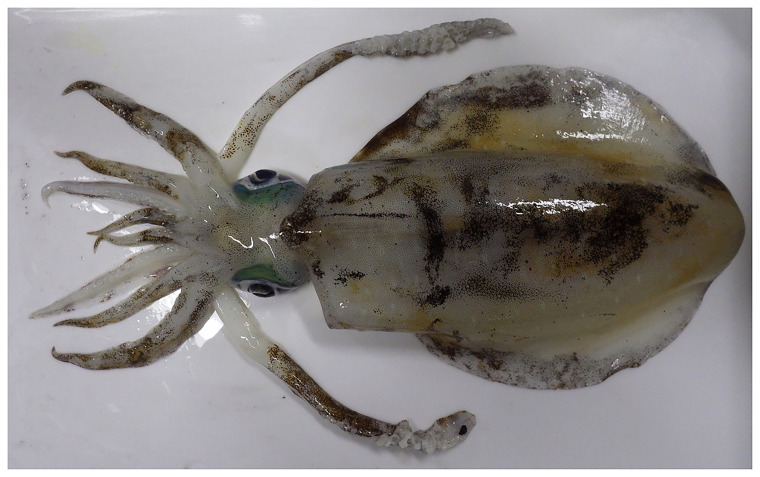 Figure 1
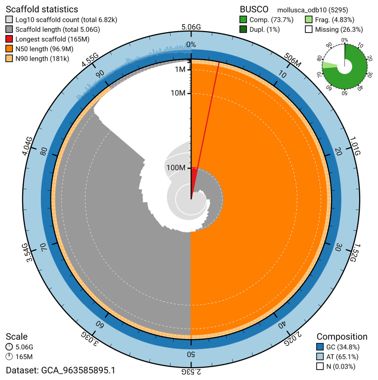 Figure 2
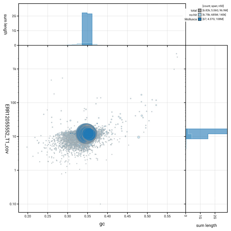 Figure 3
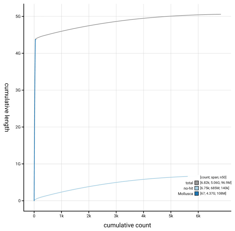 Figure 4
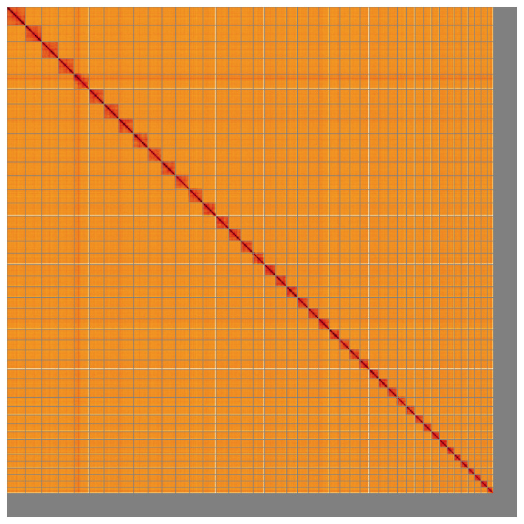 Figure 5
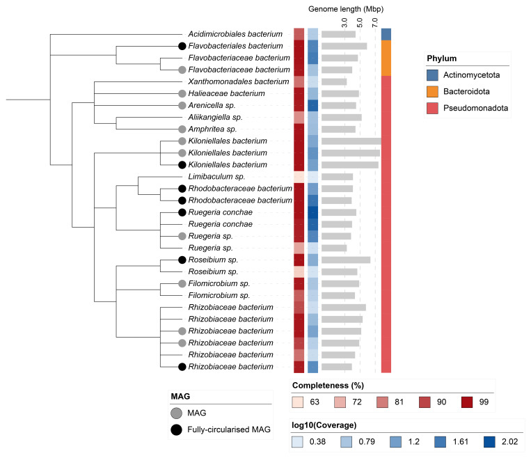 Figure 6
| Project information | |||
|---|---|---|---|
|
| Sepioteuthis lessoniana (bigfin reef squid) | ||
|
| PRJEB64979 | ||
|
|
| ||
|
| SAMEA11646235 | ||
|
| 34570 | ||
| Specimen information | |||
|
|
|
|
|
|
| xcSepLess1 | SAMEA11646288 | Somatic tissue |
|
| xcSepLess2 | SAMEA11646318 | Somatic tissue |
|
| xcSepLess2 | SAMEA11646297 | Gill |
| Sequencing information | |||
|
|
|
|
|
|
| ERR11837536 | 3.61e+09 | 545.23 |
|
| ERR11837535 | 4.36e+09 | 658.36 |
|
| ERR11843445 | 2.75e+06 | 19.73 |
|
| ERR11843447 | 2.69e+06 | 22.08 |
|
| ERR11843448 | 2.63e+06 | 25.16 |
|
| ERR11843449 | 2.64e+06 | 23.25 |
|
| ERR11843451 | 2.88e+06 | 19.13 |
|
| ERR12055552 | 8.23e+06 | 69.17 |
|
| ERR11843446 | 2.94e+06 | 20.88 |
|
| ERR11843450 | 2.93e+06 | 21.37 |
|
| ERR11843452 | 2.49e+06 | 29.14 |
|
| ERR13093641 | 1.36e+08 | 20.58 |
|
| ERR11837537 | 4.42e+07 | 6.68 |
| Genome assembly | ||
|---|---|---|
| Assembly name | xcSepLess1.1 | |
| Assembly accession | GCA_963585895.1 | |
|
|
| |
| Assembly level for primary assembly | chromosome | |
| Span (Mb) | 5,056.23 | |
| Number of contigs | 13,916 | |
| Number of scaffolds | 6,819 | |
| Longest scaffold (Mb) | 165.03 | |
| Assembly metric | Measure |
|
| Contig N50 length | 0.66 Mb |
|
| Scaffold N50 length | 96.87 Mb |
|
| Consensus quality (QV) | Primary: 51.5; alternate: 52.7; combined 52.0 |
|
|
| Primary: 84.36%; alternate: 81.77%; combined: 94.54% |
|
| BUSCO
| C:73.7%[S:72.7%,D:1.0%],F:4.8%,M:21.4%,n:5,295 |
|
| Percentage of assembly assigned to chromosomes | 86.38% |
|
| Organelles | Mitochondrial genome: 16.64 kb |
|
| Genome annotation of assembly GCA_963585895.1 at Ensembl | ||
| Number of protein-coding genes | 28,970 | |
| Number of non-coding genes | 21,583 | |
| Number of gene transcripts | 68,971 | |
| INSDC accession | Name | Length (Mb) | GC% |
|---|---|---|---|
| 1 | 165.03 | 34.5 | |
| 2 | 148.29 | 34.5 | |
| 3 | 146.83 | 34.5 | |
| 4 | 143.61 | 34.5 | |
| 5 | 135.24 | 35 | |
| 6 | 133.26 | 35 | |
| 7 | 133.09 | 35 | |
| 8 | 131.98 | 34.5 | |
| 9 | 131.16 | 34.5 | |
| 10 | 124.05 | 34.5 | |
| 11 | 122.65 | 35 | |
| 12 | 122.42 | 35 | |
| 13 | 122.24 | 34.5 | |
| 14 | 117.8 | 35 | |
| 15 | 114.22 | 35 | |
| 16 | 111.07 | 35 | |
| 17 | 108.32 | 34.5 | |
| 18 | 101.85 | 35 | |
| 19 | 101.23 | 35.5 | |
| 20 | 97.57 | 35 | |
| 21 | 96.87 | 35 | |
| 22 | 96.03 | 35 | |
| 23 | 95.44 | 35.5 | |
| 24 | 95.42 | 35 | |
| 25 | 93.84 | 35 | |
| 26 | 90.61 | 34.5 | |
| 27 | 89.63 | 35 | |
| 28 | 84.68 | 35.5 | |
| 29 | 84.74 | 35.5 | |
| 30 | 83.72 | 35 | |
| 31 | 82.93 | 35 | |
| 32 | 80.29 | 35 | |
| 33 | 78.34 | 35 | |
| 34 | 78.08 | 35 | |
| 35 | 71.07 | 35 | |
| 36 | 70.69 | 35.5 | |
| 37 | 68.51 | 35.5 | |
| 38 | 63.29 | 35.5 | |
| 39 | 62.91 | 35.5 | |
| 40 | 62.5 | 35.5 | |
| 41 | 58.21 | 35.5 | |
| 42 | 57.4 | 35 | |
| 43 | 57.12 | 35.5 | |
| 44 | 53.38 | 35 | |
| MT | 0.02 | 29 |
| NCBI taxon | Taxid | GTDB taxonomy | Quality | Size (bp) | Contigs | Circular | Mean coverage | Completeness (%) | Contamination (%) |
|---|---|---|---|---|---|---|---|---|---|
| Ruegeria sp. | 259304 | g__Ruegeria | High | 3,805,421 | 1 | No | 29.78 | 97.34 | 0.53 |
| Rhodobacteraceae bacterium | 157276 | g__SZUA-547 | High | 3,886,458 | 1 | Yes | 46.65 | 99.6 | 0.6 |
| Rhizobiaceae bacterium | 271151 | f__Rhizobiaceae | High | 3,917,026 | 1 | Yes | 25.66 | 97.91 | 1.23 |
| Ruegeria conchae | 981384 | s__Ruegeria conchae | High | 3,942,089 | 1 | Yes | 66.83 | 97.66 | 0.32 |
| Flavobacteriaceae bacterium | 165436 | g__SMXJ01 | High | 3,961,667 | 3 | No | 6.69 | 98.76 | 0.41 |
| Rhodobacteraceae bacterium | 157276 | g__SZUA-547 | High | 4,052,132 | 1 | Yes | 16.84 | 99.6 | 0.6 |
| Amphritea sp. | 981605 | g__Amphritea | High | 4,385,521 | 2 | No | 7.67 | 99.29 | 1 |
| Arenicella sp. | 1586337 | g__Arenicella | High | 4,474,314 | 19 | Partial | 65.39 | 98.17 | 0.61 |
| Ruegeria conchae | 981384 | s__Ruegeria conchae | High | 4,502,159 | 2 | Yes | 104.23 | 99.49 | 0.43 |
| Halieaceae bacterium | 2735679 | f__Halieaceae | High | 4,838,237 | 1 | No | 8.96 | 98.7 | 1.99 |
| Filomicrobium sp. | 293328 | g__Filomicrobium | High | 4,869,283 | 35 | Partial | 6.22 | 98.39 | 2.35 |
| Rhizobiaceae bacterium | 271151 | f__Rhizobiaceae | High | 4,883,131 | 32 | No | 4.87 | 91.73 | 2.09 |
| Rhizobiaceae bacterium | 271151 | f__Rhizobiaceae | High | 5,142,339 | 7 | No | 14.59 | 98.8 | 4.78 |
| Flavobacteriales bacterium | 213322 | o__Flavobacteriales | High | 5,895,559 | 1 | Yes | 29.94 | 99.73 | 1.34 |
| Roseibium sp. | 1936171 | g__Roseibium | High | 6,353,716 | 1 | Yes | 10.96 | 99.58 | 0.63 |
| Kiloniellales bacterium | 1667039 | g__JACOMY01 | High | 7,402,078 | 1 | Yes | 15.46 | 99.57 | 0.87 |
| Kiloniellales bacterium | 1667039 | g__JACOMY01 | High | 7,596,607 | 1 | No | 21.94 | 99.57 | 0.43 |
| Kiloniellales bacterium | 1667039 | g__JACOMY01 | High | 7,789,244 | 1 | No | 13.27 | 99.57 | 0.22 |
| Xanthomonadales bacterium | 412058 | f__SZUA-36 | Medium | 3,248,922 | 30 | No | 3.55 | 83.14 | 0.91 |
| Ruegeria sp. | 259304 | s__Ruegeria sp003443535 | Medium | 3,249,342 | 27 | No | 3.29 | 74.63 | 0 |
| Limibaculum sp. | 2036014 | g__Limibaculum | Medium | 4,064,720 | 170 | No | 2.4 | 63.37 | 1.2 |
| Filomicrobium sp. | 293328 | g__Filomicrobium | Medium | 4,321,939 | 42 | No | 4.53 | 86.38 | 1.81 |
| Rhizobiaceae bacterium | 271151 | g__JAALLB01 | Medium | 4,339,548 | 49 | No | 3.58 | 83.5 | 1.34 |
| Acidimicrobiales bacterium | 310071 | f__Bin134 | Medium | 4,404,047 | 14 | No | 5.15 | 87.18 | 2.99 |
| Roseibium sp. | 1936171 | g__Roseibium | Medium | 4,625,544 | 74 | No | 2.97 | 67.24 | 3.45 |
| Flavobacteriaceae bacterium | 165436 | g__GCA-2733415 | Medium | 4,710,532 | 7 | No | 36.9 | 99.53 | 7.38 |
| Aliikangiella sp. | 1920244 | g__Aliikangiella | Medium | 5,204,448 | 13 | No | 7.08 | 78.38 | 0.27 |
| Rhizobiaceae bacterium | 271151 | f__Rhizobiaceae | Medium | 5,326,527 | 32 | No | 8.06 | 98.8 | 5.26 |
| Rhizobiaceae bacterium | 271151 | g__SPNT01 | Medium | 5,757,256 | 129 | Partial | 3.41 | 89.74 | 8.83 |
| Software tool | Version | Source |
|---|---|---|
| BEDTools | 2.30.0 |
|
| bin3C | 0.3.3 |
|
| BLAST | 2.14.0 |
|
| BlobToolKit | 4.3.9 |
|
| BUSCO | 5.5.0 |
|
| bwa-mem2 | 2.2.1 |
|
| CheckM | 1.2.1 |
|
| Cooler | 0.8.11 |
|
| DIAMOND | 2.1.8 |
|
| dRep | 3.4.0 |
|
| fasta_windows | 0.2.4 |
|
| FastK | 427104ea91c78c3b8b8b49f1a7d6bbeaa869ba1c |
|
| Gfastats | 1.3.6 |
|
| GoaT CLI | 0.2.5 |
|
| GTDB-TK | 2.3.2 |
|
| Hifiasm | 0.19.5-r587 |
|
| HiGlass | 44086069ee7d4d3f6f3f0012569789ec138f42b84aa44357826c0b6753eb28de |
|
| MaxBin | 2.7 |
|
| MerquryFK | d00d98157618f4e8d1a9190026b19b471055b22e |
|
| MetaBat2 | 2.15-15-gd6ea400 |
|
| MetaTOR | - |
|
| Minimap2 | 2.24-r1122 |
|
| MitoHiFi | 2 |
|
| MultiQC | 1.14, 1.17, and 1.18 |
|
| Nextflow | 23.04.1 |
|
| PretextView | 0.2.5 |
|
| PROKKA | 1.14.5 |
|
| purge_dups | 1.2.3 |
|
| samtools | 1.19.2 |
|
| sanger-tol/ascc | - |
|
| sanger-tol/blobtoolkit | 0.4.0 |
|
| Seqtk | 1.3 |
|
| Singularity | 3.9.0 |
|
| TreeVal | 1.2.0 |
|
| YaHS | 1.1a.2 |
|
- —Wellcome Trust
- —Gordon and Betty Moore Foundation
- —Japan Society for the Promotion of Science (JSPS)
Peer Reviews
No public reviews on file for this paper yet. If you reviewed it on a platform where reviews are public (OpenReview, ICLR, NeurIPS, ICML), you can paste yours below so the community can read it here.
Videos
No videos yet. Explain this paper in a talk, walkthrough, or lecture? Add one.
Taxonomy
TopicsCephalopods and Marine Biology · Chemical synthesis and alkaloids
Species taxonomy
Eukaryota; Opisthokonta; Metazoa; Eumetazoa; Bilateria; Protostomia; Spiralia; Lophotrochozoa; Mollusca; Cephalopoda; Coleoidea; Decapodiformes; Myopsida; Loliginidae; Sepioteuthis; Sepioteuthis lessoniana d'Orbigny, 1826 (NCBI:txid34570)
Background
The bigfin reef squid Sepioteuthis lessoniana Férussac, 1831 in Lesson (1830–1831) is a demersal neritic species that belongs the Order Myopsida and the Family Loliginidae. S. lessoniana is a species complex with three lineages distributed across the coast of the Indo-Pacific Ocean, from the western Indian Ocean in the Red Sea to the Central Pacific Ocean (Hawaii) ( Cheng et al., 2014). In Japanese waters, three cryptic species have been identified based on COI sequences, allozyme electrophoresis patterns and morphology, referred to as the “aka,” “shiro,” and “kua” types ( Imai & Aoki, 2012; Tomano et al., 2016). These types correspond to Sepioteuthis sp. 1, sp. 2, and sp. 3, respectively, which represent the three distinct lineages found throughout the entire distribution of the S. lessoniana sensu stricto. The “aka” and “shiro” types are abundant off mainland Japanese waters, while the “kua,” “shiro,” and “aka” types are all found in the waters of the Ryukyu Archipelago. In addition, the “kua” type is absent from mainland Japanese waters, while the “shiro” type is the most dominant species in mainland Japan.
Hatchlings of Sepioteuthis sp. 2 are larger and more developed than any other loliginids. This advanced development has enabled successful culturing of this species over several generations ( Arnold, 1990; Shigeno et al., 2001), the study of social behaviour such as schooling ( Sakurai & Ikeda, 2024; Sugimoto et al., 2013; Sugimoto & Ikeda, 2012) and camouflage ( Nakajima et al., 2022). A reference genome for this species will facilitate comparative genomics in the Myopsida Order, enable research into the neural mechanisms underlying social behaviour, and support selective breeding through genotyping, ultimately advancing aquaculture practices.
Genome sequence report
Sequencing data
The genome of a specimen of Sepioteuthis lessoniana ( Figure 1) was sequenced using Pacific Biosciences single-molecule HiFi long reads, generating 249.90 Gb from 30.19 million reads. Based on the estimated genome size, the sequencing data provided approximately 34× coverage of the genome. Chromosome conformation Hi-C data produced 1,203.59 Gb from 7,970.82 million reads. RNA sequencing data were also generated and are available in public sequence repositories. Table 1 summarises the specimen and sequencing information.
Photograph of the Sepioteuthis lessoniana (xcSepLess1) specimen used for genome sequencing.(Photo Credits to Dr Satoshi Tomano.)
Table 1.: Specimen and sequencing data for Sepioteuthis lessoniana.
Assembly statistics
The primary haplotype was assembled, and contigs corresponding to an alternate haplotype were also deposited in INSDC databases. The assembly was improved by manual curation, which corrected 577 misjoins or missing joins and removed 3 haplotypic duplications. These interventions reduced the total assembly length by 0.35%, decreased the scaffold count by 4.09%, and increased the scaffold N50 by 14.75%. The final assembly has a total length of 5,056.23 Mb in 6,819 scaffolds, with 7,097 gaps, and a scaffold N50 of 96.87 Mb ( Table 2).
Table 2.: Genome assembly data for Sepioteuthis lessoniana.
The snail plot in Figure 2 provides a summary of the assembly statistics, indicating the distribution of scaffold lengths and other assembly metrics. Figure 3 shows the distribution of scaffolds by GC proportion and coverage. Figure 4 presents a cumulative assembly plot, with separate curves representing different scaffold subsets assigned to various phyla, illustrating the completeness of the assembly.
Genome assembly of Sepioteuthis lessoniana, xcSepLess1.1: metrics.The BlobToolKit snail plot provides an overview of assembly metrics and BUSCO gene completeness. The circumference represents the length of the whole genome sequence, and the main plot is divided into 1,000 bins around the circumference. The outermost blue tracks display the distribution of GC, AT, and N percentages across the bins. Scaffolds are arranged clockwise from longest to shortest and are depicted in dark grey. The longest scaffold is indicated by the red arc, and the deeper orange and pale orange arcs represent the N50 and N90 lengths. A light grey spiral at the centre shows the cumulative scaffold count on a logarithmic scale. A summary of complete, fragmented, duplicated, and missing BUSCO genes in the mollusca_odb10 set is presented at the top right. An interactive version of this figure is available at https://blobtoolkit.genomehubs.org/view/GCA_963585895.1/dataset/GCA_963585895.1/snail.
Genome assembly of Sepioteuthis lessoniana, xcSepLess1.1: BlobToolKit GC-coverage plot.Blob plot showing sequence coverage (vertical axis) and GC content (horizontal axis). The circles represent scaffolds, with the size proportional to scaffold length and the colour representing phylum membership. The histograms along the axes display the total length of sequences distributed across different levels of coverage and GC content. An interactive version of this figure is available at https://blobtoolkit.genomehubs.org/view/GCA_963585895.1/dataset/GCA_963585895.1/blob.
Genome assembly of Sepioteuthis lessoniana, xcSepLess1.1: BlobToolKit cumulative sequence plot.The grey line shows cumulative length for all scaffolds. Coloured lines show cumulative lengths of scaffolds assigned to each phylum using the buscogenes taxrule. An interactive version of this figure is available at https://blobtoolkit.genomehubs.org/view/GCA_963585895.1/dataset/GCA_963585895.1/cumulative.
Most of the assembly sequence (86.38%) was assigned to 44 chromosomal-level scaffolds. These chromosome-level scaffolds, confirmed by Hi-C data, are named according to size ( Figure 5; Table 3). During curation, it was noted that a large amount of repeat sequences could not be placed on chromosomes.
Genome assembly of Sepioteuthis lessoniana, xcSepLess1.1: Hi-C contact map of the xcSepLess1.1 assembly, visualised using HiGlass.Chromosomes are shown in order of size from left to right and top to bottom. An interactive version of this figure may be viewed at https://genome-note-higlass.tol.sanger.ac.uk/l/?d=RfIiARSCSauoz1ZtvLxtng.
Table 3.: Chromosomal pseudomolecules in the genome assembly of Sepioteuthis lessoniana, xcSepLess1.
The mitochondrial genome was also assembled. This sequence is included as a contig in the multifasta file of the genome submission and as a standalone record in GenBank.
Assembly quality metrics
The estimated Quality Value (QV) and k-mer completeness metrics, along with BUSCO completeness scores, were calculated for each haplotype and the combined assembly. The QV reflects the base-level accuracy of the assembly, while k-mer completeness indicates the proportion of expected k-mers identified in the assembly. BUSCO scores provide a measure of completeness based on benchmarking universal single-copy orthologues.
The combined primary and alternate assemblies achieve an estimated QV of 52.0. The k-mer completeness is 84.36% for the primary haplotype and 81.77% for the alternate haplotype; and 94.54% for the combined primary and alternate assemblies. BUSCO v.5.5.0 analysis using the mollusca_odb10 reference set ( n = 5,295) identified 73.7% of the expected gene set (single = 72.7%, duplicated = 1.0%).
Metagenome report
Twenty-nine binned genomes were generated from the metagenome assembly, of which 17 were classified as high-quality metagenome assembled genomes (MAGs) (see methods). The completeness values for these assemblies range from approximately 63% to 100% with contamination below 9%. A cladogram of the binned metagenomes is shown in Figure 6. For details on binned genomes see Table 4.
Cladogram showing the taxonomic placement of metagenome bins, constructed using NCBI taxonomic identifiers with taxonomizr and annotated in iTOL. Colours indicate phylum-level taxonomy. Additional tracks show sequencing coverage (log₁₀), genome size (Mbp), and completeness. Bins that meet the criteria for MAGs are marked with a grey circle; fully circularised MAGs are marked in black.
Genome annotation report
The Sepioteuthis lessoniana genome assembly (GCA_963585895.1) was annotated at the European Bioinformatics Institute (EBI) on Ensembl Rapid Release. The resulting annotation includes 68,971 transcribed mRNAs from 28,970 protein-coding and 21,583 non-coding genes ( Table 2; https://beta.ensembl.org/species/f1e0d42d-d087-4e33-b0af-a3606c35ba3b). The average transcript length is 27,933.39, with 1.36 coding transcripts per gene and 4.95 exons per transcript.
Methods
Sample acquisition
The specimen used for genome sequencing, one female of Sepioteuthis sp. 2, the “shiro” type (specimen ID VIEC0000008, ToLID xcSepLess1), was collected using jigging off Tosa Bay in Kochi Prefecture on 2021-04-23. The specimen was shipped frozen at –20 °C to Hiroshima University. The muscle mantle of this specimen was preserved in a 2mL Eppendorf tube and kept at –20 °C.
The specimen used for Hi-C and RNA sequencing (specimen ID VIEC0000009, ToLID xcSepLess2) was an adult specimen collected from Shimane Prefecturen, Hamada, Japan on 2021-05-21 by jigging. The specimens were collected and identified by Gustavo Sanchez (Hiroshima University).
Nucleic acid extraction
The workflow for high molecular weight (HMW) DNA extraction at the Wellcome Sanger Institute (WSI) Tree of Life Core Laboratory includes a sequence of procedures: sample preparation and homogenisation, DNA extraction, fragmentation and purification. Detailed protocols are available on protocols.io ( Denton et al., 2023). The xcSepLess1 sample was prepared for DNA extraction by weighing and dissecting it on dry ice ( Jay et al., 2023). Tissue from the muscle tissue was cryogenically disrupted using the Covaris cryoPREP ^®^ Automated Dry Pulverizer ( Narváez-Gómez et al., 2023). HMW DNA was extracted using the Automated MagAttract v2 protocol ( Oatley et al., 2023). DNA was sheared into an average fragment size of 12–20 kb in a Megaruptor 3 system ( Bates et al., 2023). Sheared DNA was purified by solid-phase reversible immobilisation, using AMPure PB beads to eliminate shorter fragments and concentrate the DNA ( Strickland et al., 2023). The concentration of the sheared and purified DNA was assessed using a Nanodrop spectrophotometer and Qubit Fluorometer using the Qubit dsDNA High Sensitivity Assay kit. Fragment size distribution was evaluated by running the sample on the FemtoPulse system.
RNA was extracted from gill tissue of xcSepLess2 in the Tree of Life Laboratory at the WSI using the RNA Extraction: Automated MagMax™ mirVana protocol ( do Amaral et al., 2023). The RNA concentration was assessed using a Nanodrop spectrophotometer and a Qubit Fluorometer using the Qubit RNA Broad-Range Assay kit. Analysis of the integrity of the RNA was done using the Agilent RNA 6000 Pico Kit and Eukaryotic Total RNA assay.
Sequencing
Pacific Biosciences HiFi circular consensus DNA sequencing libraries were constructed according to the manufacturers’ instructions. DNA sequencing was performed by the Scientific Operations core at the WSI on Pacific Biosciences Sequel IIe. Tissue from the somatic tissue of the xcSepLess2 sample was processed for Hi-C sequencing at the WSI Scientific Operations core, using the Arima-HiC v2 kit.and sequenced on the Illumina NovaSeq 6000 instrument. Poly(A) RNA-Seq libraries were constructed using the NEB Ultra II RNA Library Prep kit, following the manufacturer’s instructions. RNA sequencing was performed on the Illumina NovaSeq 6000 instrument.
Genome assembly, curation and evaluation
** Assembly **
Prior to assembly of the PacBio HiFi reads, a database of k-mer counts ( k = 31) was generated from the filtered reads using FastK. GenomeScope2 ( Ranallo-Benavidez et al., 2020) was used to analyse the k-mer frequency distributions, providing estimates of genome size, heterozygosity, and repeat content.
The HiFi reads were assembled using Hifiasm ( Cheng et al., 2021) with the --primary option. Haplotypic duplications were identified and removed using purge_dups ( Guan et al., 2020). The Hi-C reads were mapped to the primary contigs using bwa-mem2 ( Vasimuddin et al., 2019). The contigs were further scaffolded using the provided Hi-C data ( Rao et al., 2014) in YaHS ( Zhou et al., 2023) using the --break option for handling potential misassemblies. The scaffolded assemblies were evaluated using Gfastats ( Formenti et al., 2022), BUSCO ( Manni et al., 2021) and MERQURY.FK ( Rhie et al., 2020).
The mitochondrial genome was assembled using MitoHiFi ( Uliano-Silva et al., 2023), which runs MitoFinder ( Allio et al., 2020) and uses these annotations to select the final mitochondrial contig and to ensure the general quality of the sequence.
** Assembly curation **
The assembly was decontaminated using the Assembly Screen for Cobionts and Contaminants (ASCC) pipeline. Flat files and maps used in curation were generated via the TreeVal pipeline ( Pointon et al., 2023). Manual curation was conducted primarily in PretextView ( Harry, 2022) and HiGlass ( Kerpedjiev et al., 2018), with additional insights provided by JBrowse2 ( Diesh et al., 2023). Scaffolds were visually inspected and corrected as described by Howe et al. (2021). Any identified contamination, missed joins, and mis-joins were amended, and duplicate sequences were tagged and removed. The curation process is documented at https://gitlab.com/wtsi-grit/rapid-curation.
** Assembly quality assessment **
The Merqury.FK tool ( Rhie et al., 2020), run in a Singularity container ( Kurtzer et al., 2017), was used to evaluate k-mer completeness and assembly quality for the primary and alternate haplotypes using the k-mer databases ( k = 31) that were computed prior to genome assembly. The analysis outputs included assembly QV scores and completeness statistics.
A Hi-C contact map was produced for the final version of the assembly. The Hi-C reads were aligned using bwa-mem2 ( Vasimuddin et al., 2019) and the alignment files were combined using SAMtools ( Danecek et al., 2021). The Hi-C alignments were converted into a contact map using BEDTools ( Quinlan & Hall, 2010) and the Cooler tool suite ( Abdennur & Mirny, 2020). The contact map is visualised in HiGlass ( Kerpedjiev et al., 2018).
The blobtoolkit pipeline is a Nextflow port of the previous Snakemake Blobtoolkit pipeline ( Challis et al., 2020). It aligns the PacBio reads in SAMtools and minimap2 ( Li, 2018) and generates coverage tracks for regions of fixed size. In parallel, it queries the GoaT database ( Challis et al., 2023) to identify all matching BUSCO lineages to run BUSCO ( Manni et al., 2021). For the three domain-level BUSCO lineages, the pipeline aligns the BUSCO genes to the UniProt Reference Proteomes database ( Bateman et al., 2023) with DIAMOND blastp ( Buchfink et al., 2021). The genome is also divided into chunks according to the density of the BUSCO genes from the closest taxonomic lineage, and each chunk is aligned to the UniProt Reference Proteomes database using DIAMOND blastx. Genome sequences without a hit are chunked using seqtk and aligned to the NT database with blastn ( Altschul et al., 1990). The blobtools suite combines all these outputs into a blobdir for visualisation.
The blobtoolkit pipeline was developed using nf-core tooling ( Ewels et al., 2020) and MultiQC ( Ewels et al., 2016), relying on the Conda package manager, the Bioconda initiative ( Grüning et al., 2018), the Biocontainers infrastructure ( da Veiga Leprevost et al., 2017), as well as the Docker ( Merkel, 2014) and Singularity ( Kurtzer et al., 2017) containerisation solutions.
Table 5 contains a list of relevant software tool versions and sources.
Genome annotation
The Ensembl Genebuild annotation system ( Aken et al., 2016) was used to generate annotation for the Sepioteuthis lessoniana assembly (GCA_963585895.1) in Ensembl Rapid Release at the EBI. Annotation was created primarily through alignment of transcriptomic data to the genome, with gap filling via protein-to-genome alignments of a select set of proteins from UniProt ( UniProt Consortium, 2019).
Metagenome assembly
The metagenome assembly was generated using MetaMDBG ( Benoit et al., 2024) and binned using MetaBAT2 ( Kang et al., 2019), MaxBin ( Wu et al., 2014), bin3C ( DeMaere & Darling, 2019), and MetaTOR. The resulting bin sets of each binning algorithm were optimised and refined using MAGScoT ( Rühlemann et al., 2022). PROKKA ( Seemann, 2014) was used to identify tRNAs and rRNAs in each bin, CheckM ( Parks et al., 2015) (checkM_DB release 2015-01-16) was used to assess bin completeness/contamination, and GTDB-TK ( Chaumeil et al., 2022) (GTDB release 214) was used to taxonomically classify bins. Taxonomic replicate bins were identified using dRep ( Olm et al., 2017) with default settings (95% ANI threshold). The final bin set was filtered for bacteria and archaea. All bins were assessed for quality and categorised as metagenome-assembled genomes (MAGs) if they met the following criteria: contamination ≤ 5%, presence of 5S, 16S, and 23S rRNA genes, at least 18 unique tRNAs, and either ≥ 90% completeness or ≥ 50% completeness with fully circularised chromosomes. Bins that did not meet these thresholds, or were identified as taxonomic replicates of MAGs, were retained as ‘binned metagenomes’ provided they had ≥ 50% completeness and ≤ 10% contamination. A cladogram based on NCBI taxonomic assignments was generated using the ‘taxonomizr’ package in R. The tree was visualised and annotated using iTOL ( Letunic & Bork, 2024). Software tool versions and sources are given in Table 5.
Wellcome Sanger Institute – Legal and Governance
The materials that have contributed to this genome note have been supplied by a Tree of Life collaborator. The Wellcome Sanger Institute employs a process whereby due diligence is carried out proportionate to the nature of the materials themselves, and the circumstances under which they have been/are to be collected and provided for use. The purpose of this is to address and mitigate any potential legal and/or ethical implications of receipt and use of the materials as part of the research project, and to ensure that in doing so we align with best practice wherever possible. The overarching areas of consideration are:
• Ethical review of provenance and sourcing of the material
• Legality of collection, transfer and use (national and international)
Each transfer of samples is undertaken according to a Research Collaboration Agreement or Material Transfer Agreement entered into by the Tree of Life collaborator, Genome Research Limited (operating as the Wellcome Sanger Institute) and in some circumstances other Tree of Life collaborators.
The reference list from the paper itself. Each links out to its DOI / PubMed record.
- 1Abdennur N Mirny LA : Cooler: scalable storage for Hi-C data and other genomically labeled arrays. Bioinformatics. 2020;36(1):311–316. 10.1093/bioinformatics/btz 540 31290943 PMC 8205516 · doi ↗ · pubmed ↗
- 2Aken BL Ayling S Barrell D : The ensembl gene annotation system. Database (Oxford). 2016;2016: baw 093. 10.1093/database/baw 093 27337980 PMC 4919035 · doi ↗ · pubmed ↗
- 3Allio R Schomaker-Bastos A Romiguier J : Mito Finder: efficient automated large-scale extraction of mitogenomic data in target enrichment phylogenomics. Mol Ecol Resour. 2020;20(4):892–905. 10.1111/1755-0998.13160 32243090 PMC 7497042 · doi ↗ · pubmed ↗
- 4Altschul SF Gish W Miller W : Basic Local Alignment Search Tool. J Mol Biol. 1990;215(3):403–410. 10.1016/S 0022-2836(05)80360-2 2231712 · doi ↗ · pubmed ↗
- 5Arnold JM : Embryonic development of the squid.In: Gilbert, D. L., Adelman, W. J., and Arnold, J. M. (eds.) Squid as experimental animals.Boston, MA: Springer US,1990;77–90. 10.1007/978-1-4899-2489-6_6 · doi ↗
- 6Bateman A Martin MJ Orchard S : Uni Prot: the Universal Protein Knowledgebase in 2023. Nucleic Acids Res. 2023;51(D 1):D 523–D 531. 10.1093/nar/gkac 1052 36408920 PMC 9825514 · doi ↗ · pubmed ↗
- 7Bates A Clayton-Lucey I Howard C : Sanger Tree of Life HMW DNA fragmentation: diagenode Megaruptor ®3 for LI Pac Bio. protocols.io. 2023. 10.17504/protocols.io.81wgbxzq 3lpk/v 1 · doi ↗
- 8Benoit G Raguideau S James R : High-quality metagenome assembly from long accurate reads with meta MDBG. Nat Biotechnol. 2024;42(9):1378–1383. 10.1038/s 41587-023-01983-6 38168989 PMC 11392814 · doi ↗ · pubmed ↗