Contemporary hybridization among Arabis floodplain species creates opportunities for adaptation
Neda Rahnamae, Lukas Metzger, Lea Hördemann, Kevin Korfmann, Abdul Saboor Khan, Yasar Özoglan, Craig I. Dent, Samija Amar, Raúl Y. Wijfjes, Tahir Ali, Gregor Schmitz, Benjamin Stich, Aurelien Tellier, Juliette de Meaux

TL;DR
Hybridization between two Arabis species creates new genetic combinations that may help them adapt, but also brings some fitness challenges.
Contribution
The study reveals how hybridization can generate adaptive traits while identifying genomic regions linked to introgression and fitness.
Findings
Two genomic regions show strong segregation distortion favoring Arabis sagittata alleles.
A major QTL affecting flowering time implicates Terminal-Flower 1 (TFL1) as a candidate gene for adaptation.
48% of QTLs were unlinked to reduced fitness or segregation distortion.
Abstract
Hybridization between closely related species is increasingly recognized as a major source of biodiversity. Yet, whether it can create advantageous trait combinations while purging harmful alleles remains unknown. To address this question, we studied Arabis nemorensis and Arabis sagittata, two endangered species that currently hybridize in a single hotspot.We chose two representative individuals originating from the hotspot, generated high‐quality annotated genome sequences, crossed them to form an F2 population, quantified segregation distortion along the genome, measured 22 phenotypic traits and mapped their genetic basis.Two genomic regions showed strong segregation distortion favoring A. sagittata alleles in the F2 and potentially accelerating their introgression. Fifty‐eight quantitative trait loci (QTLs) were identified for 20 traits, with additive and dominance effects best…
Genes, proteins, chemicals, diseases, species, mutations and cell lines named across the full text — each resolved to its canonical identifier and authoritative record.
Click any figure to enlarge with its caption.
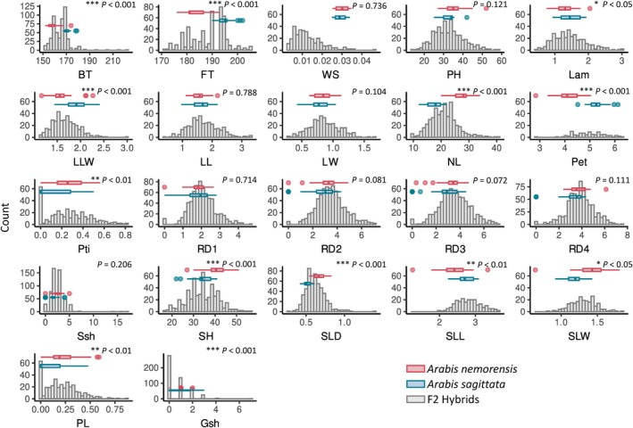 Fig. 1
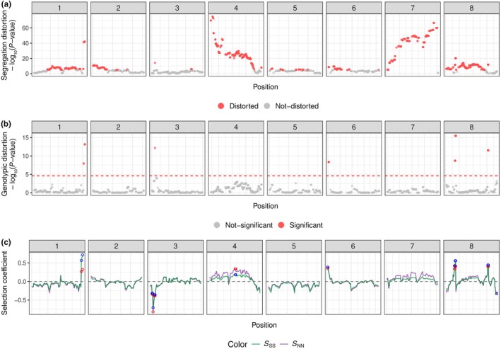 Fig. 2
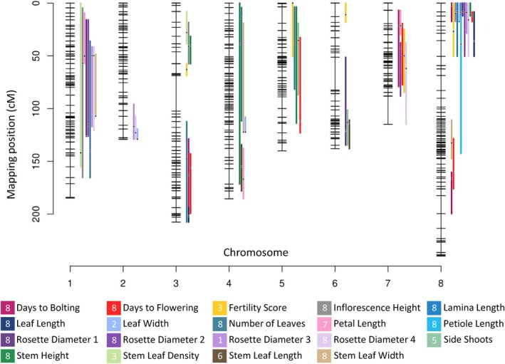 Fig. 3
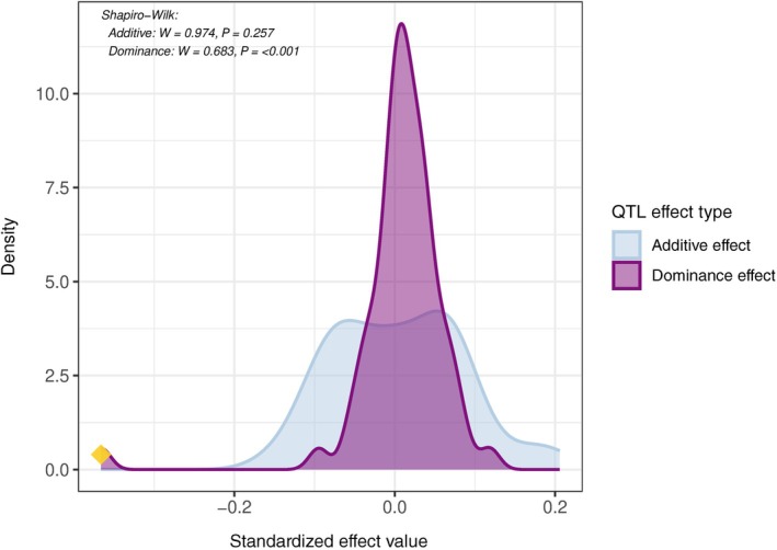 Fig. 4
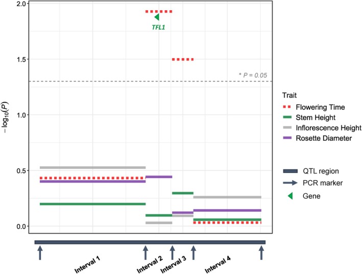 Fig. 5
| Trait | Mean | Mean | Distance |
|
|---|---|---|---|---|
| Days to Bolting (BT) (d) | 157.2857 | 169.2857 | 12 | 7.67733569186116e−29 |
| Days to Flowering (FT) (d) | 183.5714 | 193.4286 | 9.8571 | 9.92819572840268e−26 |
| Fertility Score (WS) (g) | 0.0298 | 0.0295 | 0.0004 | 0.735982604 |
| Inflorescence Height (PH) (cm) | 35.2500 | 34.5714 | 0.6786 | 0.121159231 |
| Lamina Length (Lam) (cm) | 1.2729 | 1.4646 | 0.1916 | 0.011923973 |
| Lamina L : W (LLW) (ratio) | 1.4760 | 1.7938 | 0.3178 | 3.3370726452435e−10 |
| Leaf Length (LL) (cm) | 1.5562 | 1.7161 | 0.1599 | 0.787509948 |
| Leaf Width (LW) (cm) | 0.8589 | 0.8213 | 0.0376 | 0.103685956 |
| No. of Stem Leaves (NL) | 28.1429 | 18.1429 | 10 | 2.24983890109023e−33 |
| Petal Length (Pet) (mm) | 4.0569 | 5.3579 | 1.3010 | 6.04691680241348e−34 |
| Petiole Length (Pti) (cm) | 0.2833 | 0.2516 | 0.0317 | 0.002181075 |
| Rosette Diameter 1 (RD1) (cm) | 1.8331 | 2.2419 | 0.4087 | 0.713598816 |
| Rosette Diameter 2 (RD2) (cm) | 3.2946 | 3.6893 | 0.3947 | 0.081329783 |
| Rosette Diameter 3 (RD3) (cm) | 3.3611 | 3.4424 | 0.0813 | 0.072384866 |
| Rosette Diameter 4 (RD4) (cm) | 3.8805 | 3.9110 | 0.0305 | 0.111109462 |
| Side Shoots (Ssh) (number) | 2.7857 | 2.1429 | 0.6429 | 0.205905044 |
| Stem Height (SH) (cm) | 40.4286 | 34.4286 | 6 | 3.02830254946091e−07 |
| Stem Leaf Density (SLD) (ratio) | 0.6979 | 0.5271 | 0.1707 | 3.18884502716871e−20 |
| Stem Leaf Length (SLL) (cm) | 2.3894 | 2.7921 | 0.4028 | 0.004243421 |
| Stem Leaf Width (SLW) (cm) | 1.4021 | 1.2337 | 0.1684 | 0.014377018 |
| Petiole L : Lamina L (PL) (ratio) | 0.2464 | 0.1886 | 0.0579 | 0.001013407 |
| Ground Shoots (Gsh) (number) | 0.2143 | 1.2857 | 1.0714 | 3.27306200327204e−05 |
| Trait | No. of observations | Significance of parental differences | Chr | Position (bp) | Position(cM) | LOD | %Variance explained | Est | Est |
|---|---|---|---|---|---|---|---|---|---|
| Days to Bolting (BT) | 631 | *** | 3 | 20 040 893 | 163 | 5.146 | 3.130 | 0.005914 | −0.012765 |
| 7 | 1835 566 | 21.5 | 5.359 | 3.263 | 0.010990 | 0.002648 | |||
| 8 | 2061 023 | 12.2 | 7.786 | 4.783 | −0.011989 | 0.000447 | |||
| 8 | 19 500 950 | 134.2 | 12.396 | 7.746 | 0.016244 | −0.003620 | |||
| Days to Flowering (FT) | 578 | *** | 3 | 26 882 840 | 190 | 9.915 | 4.785 | 0.012242 | −0.001815 |
| 5 | 23 418 119 | 111 | 4.868 | 2.289 | −0.007092 | 0.003427 | |||
| 7 | 1835 566 | 21.5 | 11.241 | 5.423 | 0.011243 | −0.001854 | |||
| 8 | 2061 023 | 13 | 42.112 | 23.075 | −0.021252 | 0.008320 | |||
| 8 | 18 832 553 | 133 | 9.374 | 4.488 | 0.009159 | −0.005437 | |||
| Fertility Score (WS) | 552 | 3 | 8362 080 | 63 | 8.774 | 6.165 | −0.056270 | −0.366350 | |
| 6 | 1052 484 | 10 | 3.897 | 2.683 | 0.172390 | −0.055580 | |||
| 7 | 3192 272 | 31 | 6.663 | 4.641 | 0.205690 | −0.053080 | |||
| 8 | 3118 527 | 17 | 5.070 | 3.507 | 0.178080 | −0.028820 | |||
| Inflorescence Height (PH) | 578 | . | 1 | 9004 320 | 49.9 | 4.166 | 2.385 | −0.012682 | 0.062053 |
| 3 | 2664 384 | 27 | 11.394 | 6.714 | 0.078301 | 0.016361 | |||
| 8 | 1180 103 | 6 | 20.789 | 12.728 | −0.094477 | 0.076771 | |||
| 8 | 10 128 705 | 101 | 6.383 | 3.686 | −0.062798 | −0.038649 | |||
| Lamina Length (Lam) | 436 | * | 8 | 5481 058 | 36.0 | 4.334 | 4.475 | −0.075590 | 0.042250 |
| Lamina L : W (LLW) | 436 | *** | 3 | 6744 303 | 61 | 15.635 | 14.890 | 0.089464 | −0.031374 |
| 4 | 38 897 287 | 163 | 4.045 | 3.620 | 0.041307 | 0.028487 | |||
| Leaf Length (LL) | 436 | 1 | 13 071 968 | 72.4 | 4.458 | 3.766 | 0.071867 | −0.012244 | |
| 3 | 14 255 522 | 136.2 | 5.214 | 4.423 | −0.007829 | 0.118366 | |||
| 3 | 29 031 007 | 201.4 | 5.617 | 4.775 | 0.066584 | −0.094772 | |||
| 7 | 14 342 773 | 68.8 | 4.284 | 3.615 | −0.020747 | 0.086727 | |||
| 8 | 5624 776 | 35 | 9.433 | 8.183 | −0.104748 | 0.036218 | |||
| Leaf Width (LW) | 436 | 1 | 21 722 429 | 116 | 4.313 | 3.893 | 0.069770 | 0.045460 | |
| 2 | 19 435 694 | 87 | 3.027 | 2.713 | −0.043950 | 0.056000 | |||
| 2 | 25 576 894 | 129 | 5.987 | 5.452 | 0.091250 | 0.012400 | |||
| 8 | 4356 973 | 32 | 6.705 | 6.129 | −0.081970 | 0.036770 | |||
| Number of Stem Leaves (NL) | 625 | *** | 3 | 14 075 550 | 130.9 | 4.581 | 2.557 | 0.025147 | 0.059693 |
| 4 | 7558 305 | 18 | 4.001 | 2.228 | 0.056356 | 0.010451 | |||
| 5 | 16 624 270 | 70.7 | 5.384 | 3.014 | −0.055649 | 0.004690 | |||
| 8 | 1180 103 | 7 | 28.109 | 17.139 | −0.119377 | 0.052082 | |||
| Petal Length (Pet) | 106 | *** | 1 | 9074 627 | 51 | 4.863 | 15.820 | 0.064910 | 0.039080 |
| 7 | 1835 566 | 21.5 | 5.689 | 18.850 | 0.079160 | 0.013480 | |||
| Petiole Length (Pti) | 361 | ** | 8 | 10 723 493 | 107.5 | 3.814 | 4.749 | −0.153200 | −0.035130 |
| Rosette Diameter 1 (RD1) | 695 | 1 | 17 879 753 | 95 | 4.498 | 2.747 | 0.068440 | −0.020590 | |
| 3 | 623 617 | 2.3 | 3.632 | 2.212 | 0.054350 | 0.023100 | |||
| 8 | 4362 085 | 28 | 6.942 | 4.275 | −0.074250 | 0.032990 | |||
| Rosette Diameter 2 (RD2) | 700 | . | 1 | 21 954 996 | 115 | 6.158 | 3.703 | 0.079730 | 0.013670 |
| 7 | 5769 578 | 42.7 | 3.839 | 2.291 | −0.056060 | 0.024000 | |||
| 8 | 4356 973 | 31 | 7.822 | 4.729 | −0.085450 | 0.033910 | |||
| Rosette Diameter 3 (RD3) | 696 | . | 1 | 9004 320 | 49.9 | 9.389 | 5.683 | 0.102710 | −0.005208 |
| 2 | 23 541 930 | 118 | 4.024 | 2.392 | 0.043216 | 0.071859 | |||
| 8 | 2718 077 | 18 | 7.209 | 4.332 | −0.087105 | 0.022622 | |||
| Rosette Diameter 4 (RD4) | 701 | * | 1 | 21 722 429 | 115.3 | 4.330 | 2.678 | 0.061815 | 0.014845 |
| 8 | 4356 973 | 32 | 7.814 | 4.888 | −0.078677 | 0.035138 | |||
| Side Shoots (Ssh) | 595 | * | 4 | 36 501 835 | 137.7 | 3.859 | 2.842 | −0.119930 | −0.038550 |
| 5 | 5129 643 | 35.5 | 4.875 | 3.605 | 0.126580 | 0.031450 | |||
| Stem Height (SH) | 625 | *** | 1 | 29 847 516 | 162 | 3.594 | 1.778 | −0.029247 | 0.036282 |
| 3 | 4035 375 | 36 | 13.598 | 6.984 | 0.074366 | 0.005981 | |||
| 4 | 38 897 287 | 160 | 4.386 | 2.177 | 0.042699 | −0.004189 | |||
| 8 | 1180 103 | 6 | 26.851 | 14.500 | −0.091994 | 0.070533 | |||
| 8 | 10 506 892 | 102 | 7.858 | 3.951 | −0.059677 | −0.004408 | |||
| Stem Leaf Density (SLD) | 624 | *** | 3 | 3491 752 | 29 | 5.760 | 4.162 | −0.052426 | −0.018081 |
| Stem Leaf Length (SLL) | 259 | ** | 6 | 21 070 306 | 134.8 | 5.918 | 9.356 | 0.046349 | 0.011155 |
| 8 | 3118 527 | 15 | 3.967 | 6.163 | −0.035380 | 0.011240 | |||
| Stem Leaf Width (SLW) | 259 | *** | 8 | 18 832 576 | 132.5 | 13.228 | 20.958 | −0.084603 | 0.017725 |
- —European Life Science Infrastructure for Biological Information
- —Deutsche Forschungsgemeinschaft10.13039/501100001659
Peer Reviews
No public reviews on file for this paper yet. If you reviewed it on a platform where reviews are public (OpenReview, ICLR, NeurIPS, ICML), you can paste yours below so the community can read it here.
Videos
No videos yet. Explain this paper in a talk, walkthrough, or lecture? Add one.
Taxonomy
TopicsGenetic diversity and population structure · Genetic Mapping and Diversity in Plants and Animals · Plant Molecular Biology Research
Introduction
Biodiversity is increasingly threatened by anthropogenic pressures and climate change, raising urgent questions about the mechanisms that allow species to persist (Moore & Hendry, 2009; Staudinger et al., 2012; Cochrane et al., 2016; Bontrager & Angert, 2019; Ceballos et al., 2020; Eichenberg et al., 2021; Cowie et al., 2022; IPCC, 2023; Schlaepfer & Lawler, 2023; Theissinger et al., 2023). One such mechanism is hybridization, the interbreeding of individuals from genetically distinct populations or species, which occurs frequently among close relatives (Blanckaert et al., 2023; Peñalba et al., 2024; Rosser et al., 2024). It can have both advantageous and detrimental consequences on the species receiving gene flow (Peñalba et al., 2024). First, interspecific hybridization can enable locally adapted alleles to be transferred across species barriers and thus enhance the adaptive potential of species (Seehausen, 2004; Pfennig et al., 2016; Abbott, 2017). Indeed, hybridization between populations with different ecological specializations can give rise to new, viable, and fertile hybrids equipped with novel trait combinations. Such combinations may improve the fitness of the population or even enable previously untapped habitats to be colonized (Buerkle et al., 2000; Rieseberg et al., 2003; Mallet, 2007; Abbott et al., 2013; Blanckaert et al., 2023). Hybridization can therefore have positive effects by providing a mechanism for fast evolutionary rescue (Becker et al., 2013; Todesco et al., 2020; Brauer et al., 2023; Nocchi et al., 2023).
However, the detrimental effects of hybridization are often more readily detected than its advantageous effects. Indeed, allelic incompatibilities can cause a massive fitness breakdown, when gene pools reunite after long periods of evolution in isolation (e.g. Wang et al., 2015; Cooper et al., 2018; Zuellig & Sweigart, 2018; Coughlan & Matute, 2020; Li et al., 2022; Moran et al., 2024). The overall fitness of the hybridizing population will be reduced if too many resources are used to produce poorly performing hybrids (Rhymer & Simberloff, 1996; Goulet et al., 2017). This phenomenon, sometimes described as ‘demographic swamping’, elevates the risk of extinction but may also select for allelic variations that reinforce species isolation (Hopkins, 2013; Goulet et al., 2017; Ma et al., 2019; Brauer et al., 2023).
Despite the interest in the positive consequences of hybridization and the abundant evidence for allelic incompatibilities (Bomblies & Weigel, 2007), we know little about how the positive and negative effects of hybridization interact, much less about how a genotype carrying adaptive alleles might emerge – especially against a background in which detrimental effects have been recombined out. Such ‘super genotypes’, although rare in the offspring of the first generation of hybrids (many of which may perform poorly), may represent new and exceptional combinations of adaptive alleles that, in selfing species, can determine the evolutionary success of hybridization. In addition, much focus has been placed on showing that introgressed alleles bring adaptive advantages to the recipient species (Edelman & Mallet, 2021). Yet, the role that natural selection has played in shaping the introgressing alleles of the donor species has seldom been examined. Addressing these two challenges is best achieved when hybridization can be studied as it proceeds, as this allows direct observation of the recombination and selection dynamics shaping introgression.
Here, we focused on a hybridization hotspot located along the banks of the Rhine River near Mainz, Germany, where two endangered Arabis species hybridize in a floodplain meadow (Dittberner et al., 2019, 2022). Arabis nemorensis, a perennial species within the Brassicaceae family (Arabis hirsuta tribe), inhabits floodplain meadows and is currently in a critical state in Central Europe, requiring special attention from conservation authorities (Schnittler & Günther, 1999; Burmeier et al., 2011). Arabis nemorensis is self‐pollinating and exhibits low levels of nucleotide diversity. Its endangered status is further intensified by its unique ecological requirements, and the loss of its natural habitat (Hölzel, 2005; Burmeier et al., 2011; Mathar et al., 2015; Dittberner et al., 2019). Arabis sagittata, another member of the same phylogenetic tribe (Karl & Koch, 2014), also perennial, is morphologically very similar but commonly found in calcareous grasslands and thus possibly more tolerant to drought (Dittberner et al., 2022). Arabis sagittata was recently observed in floodplains, where it naturally hybridizes with A. nemorensis (Dittberner et al., 2019, 2022). Both species mostly self in nature, although A. sagittata seems to experience rare outcrossing events more often (Dittberner et al., 2022).
Introgression analysis has revealed that gene flow between A. nemorensis and A. sagittata has happened in the past, but contemporary hybridization is restricted to the sympatric population, where intraspecific genetic variation is extremely low (Dittberner et al., 2019, 2022). Additionally, population genetics analyses estimated the divergence between A. nemorensis and A. sagittata occurred c. 900 000 generations ago, with practically complete isolation after the last glaciation (Dittberner et al., 2022).
Using the F2 progeny of a cross between two representative genotypes of A. nemorensis and A. sagittata from the hybridizing hotspot, we addressed the following questions: (1) what traits differ between species and how do these differences segregate in the F2 hybrids? (2) What is the genetic architecture of interspecific differences in this hybridizing hotspot? (3) Can a new combination of ecologically relevant traits arise and establish after hybridization? (4) Do quantitative trait locus (QTL) regions enriched in genomic regions carry footprints of past selection? Our study confirmed the extent of the genetic differences underpinning phenotypic divergence between two species. In addition, we found that some F2 hybrids show extreme trait values, despite their generally lower seed production compared to parental lines. Interestingly, incompatibility QTLs have a simple genetic basis, and some ecologically relevant QTLs are independent from the incompatibility QTLs. Collectively, these results indicate that a few offspring of hybridized species may potentially harbor a genotype with a combination of properties that none of the parents have.
Materials and Methods
Common garden experiment and phenotyping
To generate the hybrids, we crossed sympatric Arabis nemorensis genotype 10 with the Arabis sagittata genotype 69, collected from the banks of the Rhine River near Mainz in Riedstadt, Hessen, Germany, in 2015 and fully sequenced (Dittberner et al., 2019, 2022). Because nucleotide diversity within the population is very low (A. nemorensis π = 4.37e−5 and A. sagittata π = 1.32e−5, synonymous sites; Dittberner et al., 2022), we assume here that differences between these genotypes will predominantly reflect differences between species. Reciprocal F1s showed fitness comparable to parents (Supporting Information Fig. S1), and F2 progeny were raised under seminatural conditions in Cologne. In total, 1204 individuals (hybrids and parental replicates) were established. More than 20 morphological and life‐history traits, including growth, flowering time, leaf morphology, stem characteristics, fitness measures, and survival under a controlled submergence treatment, were recorded between November 2018 and April 2019. Full details of plant growth, experimental setup, and trait measurement protocols are provided in Methods S1.
Phenotypic analyses
Phenotypic differences between the parental species were assessed using generalized linear models (Trait ~ Species + Tray) with false discovery rate (FDR) correction across traits. Effect sizes are reported as incidence rate ratios with 95% confidence intervals. To evaluate genetically based correlations within the F2 population, we used mixed models accounting for cross‐direction and tray effects, extracted residuals, and calculated pairwise Spearman correlations among corrected trait values. Significant correlations (α = 0.05) were used to construct a trait network, in which nodes represent traits and edges reflect positive or negative correlations. Full details of statistical models, software, and visualization procedures are provided in Methods S2 and Notes S1.
DNA extraction and RAD‐seq library construction
We extracted DNA from frozen leaf tissue using the Nucleospin® 8 Plant II protocol. Restriction‐site‐associated DNA (RAD‐seq) libraries were prepared following Dittberner et al. (2019), with 801 F2 individuals sequenced across four NovaSeq runs at the Cologne Center for Genomics. Sequencing produced between 3 and 6 million reads per individual, covering c. 2% of the 248 Mb genome. Further details of library preparation and sequencing are provided in the Methods S3.
Genome assembly, SNP calling, and linkage map construction
Chromosome‐scale genome assemblies for both parental lines were generated using PacBio HiFi and Hi‐C sequencing, scaffolded with reference‐ and linkage‐map–based approaches (ENA Project ID: PRJEB89863). Variant calling from RAD‐seq data and genetic map construction were performed using standard filtering and imputation procedures, resulting in 2082 single‐nucleotide polymorphism (SNP) markers across 742 F2 individuals. Full protocols, filtering thresholds, and software parameters are available in Methods S4 and S5, and Notes S2–S4.
Segregation distortion and selection coefficient
We assessed segregation distortion within each region by applying a test of segregation distortion (profileMark) for each marker with Bonferroni correction using the ASMap package in R. To assess deviations from the Hardy–Weinberg equilibrium (HWE) and estimate selection coefficients, allele frequencies for each genotype (NN, NS, SS) were calculated based on the total number of individuals (n = 742). The observed genotype counts were used to compute allele frequencies (FreqN and FreqS) by summing homozygous and heterozygous contributions. Expected genotype frequencies under the HWE were then computed as FreqN2 (NN), 2 × FreqN × FreqS (NS), and FreqS2 (SS). These frequencies were scaled to expected counts by multiplying by the total number of individuals (Notes S4).
To determine significant deviations from the HWE, a chi‐squared goodness‐of‐fit test was performed for each locus. The observed and expected genotype counts were compared using the chi‐squared statistic, with 2 degrees of freedom. Significant deviations were identified based on a Bonferroni‐corrected P‐value threshold, accounting for multiple testing across all loci. The Bonferroni correction was applied by adjusting the significance threshold to 0.05 divided by the total number of markers (2082); this adjustment ensured that false positives were stringently controlled. Additionally, selection coefficients (t and s) were estimated by calculating the relative differences in ratios of observed to expected frequencies among genotypes. Specifically, the coefficients were defined sNN=1−ratioNNratioNS and sSS=1−ratioSSratioNS, reflecting the relative fitness difference between homozygotes and heterozygotes (Carey & Ganders, 1980) (Notes S4).
Significance of genotype deviations from the HWE was assessed using a chi‐squared test for each marker. P‐values were adjusted for multiple testing using the FDR correction method, controlling the FDR at 5%. Markers with FDR‐adjusted P‐values below 0.05 were considered significant and were visually highlighted in the selection coefficient plot. Red and blue circles denote significant selection against NN (t) and SS (s), respectively. When both t and s were significantly greater than zero, markers were interpreted as showing potential selection favoring the heterozygote (NS).
QTL mapping
QTL analyses were conducted using the r/qtl and qtltools packages (v.1.66; Broman et al., 2003; v.1.3.1; Delaneau et al., 2017) in R. QTL mapping was performed on the residuals of the phenotypic models described above (Phenotypic Analyses), in which we had already controlled for cross‐direction (cytoplasmic effects) and TrayBlock structure (positional effects). These residuals were then used directly in genome‐wide QTL scans for 22 traits listed in Table 1. However, survival after flooding, being a binomial trait, lacked a sufficient number of F2 individuals for QTL mapping (Notes S5).
For each trait, we used the scantwo function to perform a two‐dimensional genome scan with a two‐QTL model, applying the Haley–Knott regression algorithm (Haley & Knott, 1992). Penalties were calculated from 1000 permutations of the scantwo function to support the stepwise fitting of multiple QTL models. The stepwiseqtl function was then employed, with a maximum of five QTL, using Haley–Knott regression to search for optimized models. Allowing for more QTL did not change the results. We activated the refine.locations option in stepwiseqtl to improve the localization of QTLs and deactivated the additive.only option to allow for potential interactions between QTLs in the model.
We then looked into the summary output of stepwiseqtl to obtain information on the percentage of variance explained by each QTL, as well as the peak Logarithm of the odds (LOD) scores, and the additive (a) and dominance (d) effects for each significant QTL, reported relative to the A. nemorensis (N) allele (coded as the baseline parental allele in the QTL analysis), identified in the best stepwise models for each trait. For each identified QTL, we determined the 1.5 LOD confidence interval using the lodint function in r/qtl. Finally, we used the segmentsOnMap function from qtltools to visualize QTL segments on the genetic map, and ggplot2 (v.3.5.1; Wickham, 2011) to plot QTL effect sizes using the LOD scores obtained from the summary output of stepwiseqtl. To assess the distribution of estimated additive and dominance effects across traits, we performed the Shapiro–Wilk normality test in R (Villasenor Alva & Estrada, 2009) using standardized phenotype residuals derived from a GLM that accounted for cytoplasmic and positional effects, enabling comparisons across traits (Notes S5). Because QTLs associated with fertility or segregation distortion can inflate effect size estimates, we excluded those loci from this analysis. Specifically, we removed QTLs located in known segregation distortion regions (Chromosomes 4 and 7) and QTLs whose intervals overlapped with fertility score QTLs on the same chromosome. This allowed us to focus on the distribution of effect sizes among QTLs associated with other phenotypic traits.
Analysis of whole‐genome resequencing data
We reanalyzed published whole‐genome resequencing data for 37 A. nemorensis and A. sagittata individuals, with A. androsacea as an outgroup (Dittberner et al., 2022). Reads were mapped to our new A. nemorensis reference genome, and SNP calling and filtering were performed using standard pipelines. Full details of read processing, variant calling, and filtering thresholds are provided in the Methods S6.
Genome‐wide selection scans
Using the 37 full genome samples, we identified selective sweeps using biallelic SNPs and the omegaplus software (Alachiotis et al., 2012). The OmegaPlus statistics (omega) were calculated using a grid size of 200 000 bp. We defined a minimum window size (minwin) of 50 kb and a maximum window size (maxwin) of 100 kb for computing LD values between SNPs. Outlier omega statistics, which indicated selective sweeps had occurred, were determined based on the genome‐wide distribution of values. To minimize false positives arising from demographic processes, the cutoff values for the omega statistics were established using forward simulations in SLiM4 (Haller et al., 2019; Haller & Messer, 2023) that were simulated under the demographic history inferred by Dittberner et al. (2022). In short, the demography consists of two pulses of interspecific gene flow between both species, one ancient pulse that occurred directly after the species split and one recent migration event that occurred only between the sympatric populations.
We generated 10 000 neutral datasets of 2 Mb each under the demographic history of ancient and recent migration events that occurred between the two species, assuming a fixed recombination rate for each simulated block (5.5e−8). The maximum omega value from each simulated dataset was extracted, yielding a distribution of 10 000 maximum values. The 99th percentile of this distribution that was used as the threshold to identify outlier windows indicated selective sweeps had occurred.
To optimize sweep detection, we tested multiple combinations of grid, minwin, and maxwin parameters (from 50 to 200 kb for grid size, and 50 to 100 kb for minwin and maxwin). We then applied the optimized parameters to the real dataset of A. nemorensis and A. sagittata, extracting only the sweep regions that exceeded the simulation‐based threshold, which were considered high‐confidence selective sweep regions.
We further investigated the potential association between selective sweeps and phenotypic traits by analyzing the overlap between the identified sweep regions and QTLs in A. nemorensis and A. sagittate (Notes S6). We used only high‐confidence selective sweeps in 200‐kb windows across the genome and overlaid these with the positions of all QTLs. We focused on the 10 percent quantile regions around the QTL peak positions to increase specificity.
Fine‐mapping the largest effect QTL
To fine‐map the largest effect QTL, which was associated with the Days to Flowering trait (first QTL on Chromosome 8), we identified F2 lines that were heterozygous for the QTL of interest and homozygous for other Days to Flowering QTLs; a total of 15 lines resulted (Tables S1, S2). We sowed 90 F3 seeds per line (3 seeds per pot) in trays and transferred these to the cold chamber for vernalization. After 2 wk, we transplanted one seedling into each 7 × 7 cm pot filled with Topferde (Einheitserde, Sinntal‐Altengronau, Germany), resulting in 30 seedlings per line. Pots were kept in the glasshouse for 6 wk, after which plants were transplanted into larger 9 × 9 cm pots and moved to cold frames in the garden for 7 wk. During this period, leaf material was harvested from each plant, and DNA was extracted from fresh leaves using the NucleoSpin® 8 Plant II protocol. Subsequently, the plants were transplanted into new 11 × 11 cm pots and placed on tables in the garden under a bird‐protected cage. We recorded flowering time, inflorescence height, internode length, number of shoots, plant height, stem leaf density, stem height, and rosette diameter (RD). Two successive trials were carried out on 483 plants; the first started on 26 September 2022, the second on 16 November 2022. Plants flowered between April and June 2023.
geneious prime® (v.2024.0.5) was used to design multiple species‐specific primers targeting the QTL region based on the A. nemorensis and A. sagittata genomes. We designed five pairs of PCR markers, which divided the QTL region into four intervals. PCR was conducted on the DNA of 407 plants to identify recombinants and locate their recombination events within the predefined intervals. We built a quantitative model using the glm function from the stats package (v.3.6.2) in R, accounting for both family and trial effects as fixed factors (glm(flowering_time ~ family × (exp/tray_garden), family = quasipoisson)), in which trays were nested within experiments because tray labels were reused across experiments. We included the interaction term (family × (exp/tray_garden)) because families showed variation among experiments in flowering time. Flowering time was defined as the number of days from sowing to the first open flower (days after sowing). Then, we extracted residuals and ran another model on the residuals (glm(res_ftime ~ interval1 + interval2 + interval3 + interval4, family = gaussian)). The model was run for each interval, with the interval that best explained variation in flowering time residuals containing the flowering time QTL (Notes S7). The same procedure was then applied to assess the impact of each interval on traits with overlapping QTLs in the same region as the F2 mapping population (Inflorescence Height, RD, and Stem Height). Parental DNA was used as a positive control, and nuclease‐free water (no template) was included as a negative control to monitor for contamination and confirm that amplification was specific to DNA templates.
Results
Phenotypic differences of ecologically relevant traits
In total, 1193 individuals germinated in the glasshouse and were set to grow in a common garden situated at the University of Cologne. All replicates of A. nemorensis and A. sagittata survived the common garden experiment (35 A. nemorensis and 35 A. sagittata). Arabis nemorensis flowered c. 12 d earlier than A. sagittata (P < 0.001, Table 1). Mean values for 13 of the 22 scored traits differed between species (Table 1; Notes S1).
Arabis nemorensis individuals displayed a markedly higher number of stem leaves compared to A. sagittata (mean difference = 10 leaves, P < 0.001), as expected for a trait that is often used to determine the taxonomy of these species (Titz, 1979). The RD of the parental genotypes did not differ significantly after 1, 2, 3 and 4 wk of growth (all P > 0.05). Moreover, trait variance among F2 hybrids was generally larger than trait variance between their parental genotypes, suggesting transgressive segregation (Fig. 1). Although the seed production of parents did not differ significantly (Fertility Score or WS, P = 0.735982604), the low fertility observed for most F2 contrasted with the normal fertility of F1s (Fig. S1) and indicated outbreeding depression (Fig. 1).
*Phenotype distribution in Arabis F2 progeny and their parental lines. Histograms illustrate the distribution of traits in the 1193 plants of the F2 generation grown in a common garden. Boxplots highlight trait variations between the two parental lines and indications of transgressive segregation in their offspring. The box represents the interquartile range, the horizontal line shows the median, whiskers extend to 1.5x IQR, and points beyond the whiskers are plotted as outliers. The P‐values and stars depict the significance of trait differences between parents: *, P < 0.05; **, P < 0.01; **, P < 0.001. They were obtained with generalized linear models (Trait ~ Parent + Tray). Parental contrasts were obtained via emmeans and P‐value were corrected for false discovery rate. BT, Days to Bolting; FT, Days to Flowering; Gsh, Ground Shoots; LL, Leaf Length; LW, Leaf Width; Lam, Lamina Length; LLW, Lamina Length‐to‐Width Ratio; NL, Number of Stem Leaves; PH, Inflorescence Height; PL, Petiole Length‐to‐Lamina Length Ratio; Pet, Petal Length; Pti, Petiole Length; RD1‐4, RD at four time points; SH, Stem Height; SLD, Stem Leaf Density; SLL, Stem Leaf Length; SLW, Stem Leaf Width; Ssh, Side Shoots; WS, Fertility Score – Seed Production.
After 4 wk of flooding, the survival rates of parental genotypes showed no significant differences (χ2(1, n = 14) = 0.43, P = 0.5116).
The cross‐direction impacted several traits, suggesting maternal influence and potential cytoplasmic effects (Table S3). Traits such as Stem Leaf Length (SLL, P = 3 × 10^−5^), RD at early stages (RD1, P = 8 × 10^−5^), and Petiole Length (Pti, P = 0.006) exhibited strong associations with the direction of the cross. Additionally, Petiole Length‐to‐Lamina Length Ratio (PL, P = 0.011), RD 2 (RD2, P = 0.013), and RD 3 (RD3, P = 0.03) also displayed significant maternal effects. In terms of direction, A. sagittata maternal cytoplasmic inheritance increased SLL (consistent with the larger parental SLL of A. sagittata), but decreased RDs RD1‐RD3 (opposite to the parental difference, since A. sagittata parents had larger rosettes). For Pti and PL, in which A. nemorensis parents were larger, having A. sagittata as the mother increased trait values, again opposite to the parental difference. Arabis sagittata maternal cytoplasmic inheritance decreased rosette lamina size on the rosette but increased it on the stem (Table S3; Fig. S2). Thus, maternal effects were trait‐specific, sometimes reinforcing and sometimes opposing parental trait differences. By contrast, the majority of traits, including Days to Bolting (BT), Days to Flowering (FT), Fertility Score (Seed Production or WS), and structural traits such as Inflorescence Height (PH) and Number of Stem Leaves (NL), showed no cytotype effects (P > 0.05), indicating limited or negligible maternal influence.
Spearman correlation analysis of 22 traits in the F2 population revealed relationships among traits (Figs S3, S4). Traits associated with leaf shape, such as Lamina Length (Lam) and Leaf Width (LW), exhibited strong positive correlations (r > 0.8, P < 0.001). Similarly, RD (RD1–RD4) measured at different time points showed strong positive correlations (r > 0.7, P < 0.001).
Developmental traits, such as Days to Bolting (BT) and Days to Flowering (FT), showed moderate correlations with vertical growth traits, including Stem Height (SH) and Inflorescence Height (PH). For instance, Inflorescence Height was positively correlated with Days to Flowering (r = 0.535, P < 0.001), suggesting that later‐flowering individuals allocate more resources to vertical growth. By contrast, Fertility Score (Seed Production or WS), a component of fitness, exhibited weaker and often insignificant correlations with other traits, indicating potential independence from vegetative and structural phenotypes.
Petiole traits, including Petiole Length (Pti) and its ratio to Lamina Length (PL), were moderately correlated with rosette size and leaf shape traits such as Leaf Width (LW). Overall, these findings highlight the interdependencies among structural traits (e.g. plant size, leaf shape), developmental traits (e.g. flowering time, rosette size over time), and fitness components in Arabis F2 hybrids. The statistical analyses of ecologically relevant traits in the common garden experiment provide valuable insights into the extent of phenotypic integration and the nature of resource allocation strategies in the F2 hybrid population.
Genetic map, pre‐ and postzygotic selection distortion
To investigate the genetic architecture underlying trait variation, we used a reduced sequencing approach to determine the genotypes of 742 F2 individuals at 2082 reliable SNP markers with the help of high‐quality genome assembly (Fig. S5; Notes S2), and constructed a genetic map. The map consisted of eight linkage groups (LGs), which were numbered according to the chromosome numbers of Arabis alpina. The length of the linkage map was 240 cM, with 160–369 markers per chromosome (Table S4). Contrasting the genetic and physical distances of SNPs along chromosomes showed that recombination was higher on chromosome arms compared to in centromeric regions (Figs S6, S7).
The analysis of allele and genotype frequencies along the genome uncovered strong segregation distortions in the F2 population. A strong segregation distortion was found on Chromosomes 4 and 7 with the percentage of N alleles dropping from 50% (expected) to 32% (Fig. 2a). Because the sequencing data were mapped on the high‐quality A. nemorensis genome, we can conclude that this depletion is clearly not due to mapping biases. To disentangle prezygotic from postzygotic mechanisms of allele distortion, we estimated the difference between expected and observed genotype distributions across the genome using a chi‐squared test (Fig. 2b), and inferred selection coefficients against each type of homozygote. This analysis showed that the segregation distortions on Chromosome 7 and on the tip of Chromosome 4 were not due to postzygotic selection on the genotype. Yet, it identified six regions in the genome with a significant excess of heterozygotes, three of which were particularly strong on Chromosomes 1 and 8. It further highlighted one region in Chromosome 3 with massively depleted homozygotes.
Segregation distortion, genotypic distortion and strength of selection along the genome in Arabis F2 progeny. This figure illustrates segregation distortion, genotypic distortion, and the strength of selection across the genome in the F2 population. The x‐axis represents marker positions along the genome across the eight chromosomes (2082 markers). The y‐axis in (a, b) shows −log10 (P‐value); the y‐axis in (c) represents the selection coefficient. (a) Gametic distortion: shown by the deviation of single‐nucleotide polymorphism from expected Mendelian segregation ratios, assessed using a segregation distortion test (profileMark) with Bonferroni correction for multiple testing (threshold P < 2.4 × 10⁻⁵). Significant deviations are highlighted in red. A total of 1257 markers are significantly distorted. (b) Genotypic distortion: calculated as the deviation of observed genotypes from expected values according to the Hardy–Weinberg equilibrium (HWE), assessed using a chi‐squared test. Bonferroni‐adjusted significant differences are highlighted in red. Only 47 markers surpassed the Bonferroni significance threshold. (c) Selection coefficient (s): calculated based on deviations from expected allele frequencies, with selection on allele S represented in green and on allele N in purple. Red and blue circles indicate markers where genotype frequencies significantly deviate from the HWE (false discovery rate (FDR)‐adjusted P < 0.05, chi‐squared test), suggesting selection at those loci. Red circles represent significant selection against the NN genotype (t); blue circles represent selection against the SS genotype (s). Loci where both t and s are significant and positive, indicate potential selection favoring the heterozygote (NS).
The extent of segregation distortion found throughout the genome appeared to be mostly due to interactions between alleles and not between different loci. For example, no genetic association was observed between the distortion on Chromosomes 4 and 7 (Fig. S8). Nevertheless, we find biased transmissions of parental alleles on Chromosomes 2 and 5, as well as Chromosomes 3 and 8 (Fig. S8).
Genetic architecture of ecologically relevant traits
We detected significant QTLs for 20 of the 22 traits we scored (Table 2). The number of QTLs per trait ranged from 1 (Lamina Length) to 5 (Days to Flowering). The most significant QTL (LOD score > 40) was identified on Chromosome 8, accounting for more than 20% of the variation in flowering time. By contrast, the lowest LOD score (3.027) was observed in one of the Leaf Width QTLs. In total, 58 QTLs were identified along the genome (Table 2). We observed overlapping QTLs for multiple traits, including 9 on Chromosome 1; 3 on Chromosome 2; 11 on Chromosome 3; 4 on Chromosome 4; 3 on Chromosome 5; 2 on Chromosome 6; 6 on Chromosome 7; and 20 on Chromosome 8 (Fig. 3). Notably, one QTL associated with the Fertility Score on Chromosome 6 did not overlap with any other QTLs (Fig. 3; Table 2).
Genetic map with quantitative trait loci (QTLs) for ecologically relevant traits in Arabis F2 progeny. The plot illustrates significant QTLs that were detected and located on the genetic map. Horizontal bars represent mapped single‐nucleotide polymorphism (SNP) markers. Gaps between bars stand for the genetic distance between SNP markers in cM (centimorgan). Traits are listed in alphabetical order. The chromosome containing the strongest QTL of each trait appears in the square.
The largest effect QTLs for traits such as Days to Bolting, Days to Flowering, Inflorescence Height, Leaf Length and Width, Number of Stem Leaves, and RD after 1, 2, and 4 wk, as well as Stem Height and Stem Leaf Width, were all located on Chromosome 8. Additionally, the strongest QTLs for Petal Length, RD 3, Side Shoots, Stem Leaf Density, and SLL were identified on Chromosomes 7, 1, 5, 3, and 6, respectively. For all traits, the additive effect of the A. nemorensis allele was either positive or negative, confirming that transgressive genetic variation can arise in most traits in this selfing species by fixing a new combination of alleles (Table 2).
The distribution of fertility scores, which was measured as the weight of seeds contained in 10 siliques, indicated that F2 individuals tended to be less fertile than the parental lineages. The genetic architecture of fertility score variation was dominated by a large‐effect QTL (LOD = 8.774) on Chromosome 3 (Fig. S9), which explained > 30% of the phenotypic variation and involved interallelic incompatibility at position 8 362 080 bp on Chromosome 3 (QTL interval: 6 744 303 to 9 601 991 bp; Fig. S9). Individuals with the NS heterozygous genotype at this marker displayed markedly lower fertility. In addition, three smaller QTLs explaining 2.683%, 4.641%, and 3.507% of the variation were found on Chromosomes 6, 7, and 8, respectively. It can be concluded that the genetic basis of outbreeding depression is relatively simple in this population.
Of the 22 traits scored, Ground Shoots (Gsh), Petiole Length‐to‐Lamina Length ratio (PL), and Survival to Flooding revealed no significant QTL. For two of these three traits (Ground Shoots, Petiole Length‐to‐Lamina Length ratio), significant differences between species were observed. The absence of QTLs for these traits suggests they may have a polygenic genetic basis, and the effect of individual variants may be too small to be detected.
We conclude that the two parental lineages differ genetically in many traits, with effects of various sizes. The number of detected QTLs further allowed us to describe the effect sizes of genetic variation that can be generated by hybridization in this system. The standardized additive effects were normally distributed (Shapiro–Wilk: W = 0.9744, P = 0.2573; Fig. 4), ranging from a minimum of −0.15 to a maximum of 0.20 with a median of 0.008 (mean = 0.005, SD = 0.08, skewness = 0.29, kurtosis = 2.6). QTLs with the largest effects controlled flowering time, stem height, inflorescence height, leaf number, and lamina shape contributing to the heavy tail of the distribution of additive effect (Figs 4, S10). Standardized dominance effects instead approximated a logistic distribution (Shapiro–Wilk: W = 0.683, P < 0.001), ranging from −0.36 to 0.11 with a median of 0.012 (mean = 0.008, SD = 0.062, skewness = −3.70, kurtosis = 23.5). The dominance effect of the fertility score QTL on Chromosome 3 was an outlier to this distribution (Fig. 4). Since it uses standardized phenotypic values, this distribution can help benchmark genetic variation in other studies of hybridization.
Distribution of standardized quantitative trait loci (QTL) estimated additive and dominance effects in Arabis F2 progeny. The figure displays the distribution of standardized estimated additive and dominance effects for QTLs associated with ecologically relevant traits identified in the F2 population. Each curve represents the density of standardized effect sizes for a distinct type of genetic effect: additive effects (in light blue) and dominance effects (in purple). The yellow diamond marks the dominance effect of the strongest QTL for Fertility Score (WS) on Chromosome 3. Effect values were estimated using interval mapping on standardized phenotype residuals derived from a GLM that accounted for random effects, enabling comparisons across traits. Density distributions illustrate the range and frequency of QTL contributions. Additive effects showed a Gaussian distribution (Shapiro–Wilk: W = 0.974, P = 0.257), whereas dominance effects approximated a logistic distribution after excluding the outlier dominance effect of a QTL on Chromosome 3 (Shapiro–Wilk: W = 0.683, P < 0.001).
Genes responsible for flowering time
The largest effect QTL detected in this study impacts the timing of flowering and is located on Chromosome 8, where two well‐known genes that control flowering time are found: FLC, a regulator involved in the vernalization pathway, and CONSTANS, a regulator involved in the photoperiod pathway (Andrés & Coupland, 2012). FLC has been shown to be a key variant shaping flowering time in many Brassicaceae species, including the congeneric species A. alpina (Albani et al., 2012). The gene CONSTANS is also located within the boundaries of this QTL. In order to test whether one of these candidate genes was responsible for the variation, we selected 15 F2 individuals that were heterozygous in the QTL region of Chromosome 8 and homozygous on the other QTLs, and we grew 30 of their seeds. A total of 410 plants were assessed for flowering time in 15 F3 families and two trials (Fig. S11, Tables S1, S2).
With 410 plants and a QTL region that was c. 17 cM, we expected 80 recombinants. Interestingly, we identified 138 recombinants, suggesting that the recombination rate had been slightly underestimated in the F2 population. We compared four models to identify the chromosomal fragments that best explained variation in flowering time, after accounting for all other factors of the experimental design. Using Akaike's criterion and comparing P‐values, we identified Fragment 2 as the most likely to contain the variants causing a difference in flowering time (Fig. 5, P = 0.0118). This segment ranges from position 1 831 324 bp to position 2 125 083 bp at the beginning of Chromosome 8. Although this c. 300 kb region does not contain FLC or CO, it contains 64 other genes, 31 of which have a known ortholog in Arabidopsis thaliana. Only one of these, Terminal‐Flower 1 (TFL1), is known to regulate flowering time in A. thaliana and A. alpina, with a loss of function inducing early flowering in both species (Cerise et al., 2023). Arabis sagittata TFL1 differs from the A. nemorensis copy by two amino acid exchanges: Asparagine 3 is changed to Isoleucine and Serine 50 is changed to Tyrosine. The A. nemorensis version at both sites is conserved in most Brassicaceae, like A. thaliana, where TFL1 function has been experimentally verified (Andrés & Coupland, 2012). Nevertheless, both positions are not strictly conserved.
Association between four DNA fragments and flowering time within 15 Arabis F3 families segregated for the chr8 flowering time quantitative trait loci (QTL). The figure illustrates the role of genomic intervals within the QTL region in explaining variations in Flowering Time, Inflorescence Height, Rosette Diameter, and Stem Height. The x‐axis represents the region of the strongest Flowering Time QTL, divided into intervals defined by species‐specific primers with adjusted lengths for fine‐mapping. The dashed line indicates the significance threshold. Different bar colors represent different traits. The TFL1 gene was detected in Interval 2, which shows the strongest effect on flowering time.
In contrast to most TFL1 genes from the Brassicales, several species within (Capsella rubella, Sinapis alba) and outside of this group are missing the start codon and protein translation starts at the conserved Methionine codon at Position 4. At Position 50, Serine is the most common amino acid not only in the Brassicales group but also in other plant groups; other amino acids (Alanine, Threonine, Phenylalanine) are found in other Brassicaceae TFL1 sequences. Because A. sagittata carries derived amino acids at two moderately conserved positions, gene activity may be decreased compared to the more ancestral A. nemorensis allele. However, fine‐mapping allowed us to exclude the role of flowering loci such as FLC or CO that locate on the same chromosome arm of chromosome 8.
Although there were QTLs for Inflorescence Height, RD, and Stem Height, on Chromosome 8 in F2s, the chromosomal region that was fine mapped did not explain the variation of these traits in F3s. Inflorescence Height, RD, and Stem Height are thus controlled by QTL(s) independent of the QTL for Flowering Time in the TFL1‐containing fragment, with the S allele advancing flowering compared to the N allele.
Overlap of parental QTLs with the history of selection in the parental lineages
In order to test whether genetic differences between lineages were influenced by natural selection in the two parental lineages, before hybridization, we used previously published population genomics data to determine regions with signatures of selective sweeps (Dittberner et al., 2022). We detected 35 and 82 genome regions carrying signatures of selective sweeps in A. nemorensis and A. sagittata, respectively, which prompted us to ask whether variable traits were disproportionately targeted by natural selection in their lineage or origin (Fig. S12). Many of the 58 QTL regions spanned large parts of chromosomes, sometimes overlapping with multiple independent selective sweeps (Fig. S13). We tested whether the distance between QTL peak and selective sweep was shorter than expected by a permutation test. QTL peaks did not tend to be located close to selective sweep signatures. We also did not detect significant overlaps between regions with distorted segregation and regions carrying selective sweeps (not shown). The genetic variation segregating in the F2 population thus does not appear to reflect the history of selection in the hybridizing lineages, yet some individual QTLs may reflect recent selection. For example, sweeps overlapped with five of the seven genomic regions with QTLs for rosette size (Fig. S12). By contrast, no signature of a putative selective sweep was found in the TFL1 region.
Discussion
Hybridization between species is pervasive in both past and contemporary ecosystems (Lewontin & Birch, 1966; Stull et al., 2023). By bringing together alleles that contribute to different ecological specialization, it can facilitate the emergence of a new allelic combination that may surpass the performance of the parental genotypes and be fixed via selfing. Hybridization may therefore become pivotal in the rescue of endangered selfing species with very low levels of genetic diversity (Frankham, 2015). Here, we take advantage of a hybridization hotspot we identified previously to disentangle the genomic and ecological properties of genetic variation released after hybridization; some of these properties may propagate in the population via selfing. An F2 generation was obtained by crossing individuals' representative of the two species in the sympatric population where they naturally hybridize (Dittberner et al., 2019, 2022).
The genetic analysis of allelic transmission in the F2 population first revealed the genomic barriers that skew allele segregation in hybrid offspring. Indeed, several regions of the genome displayed highly distorted transmission. For the two most strongly distorted regions on Chromosomes 4 and 7, the genotypic composition of the F2 fits Mendelian expectations, suggesting that the distortion happens before fertilization, as a result of biased gamete formation. Both of these distortions drive the A. sagittata allele to high frequencies in the F2 offspring population. We thus conclude that we observe meiotic drive in our cross, that is, the predominance of one allele among mature gametes produced in a heterozygous individual. Meiotic drive is a very strong evolutionary force (Sandler & Novitski, 1957; Pinkas et al., 1985; Clarke et al., 2004; Domínguez et al., 2005). It can massively accelerate the fixation of alleles linked to the driver locus. Driver alleles may outcompete nondriver alleles during pollen tube growth in heterozygotic selfing plants, thereby biasing the paternal transmission of alleles in favor of the offspring (e.g. Snow & Spira, 1996; Aronen et al., 2002; Lankinen et al., 2009). In female gametes, any molecular change that favors allele transmission into the polar body would lead to preferential maternal transmission (Finseth et al., 2015; Fishman & Kelly, 2015). Here, since genotype frequencies fulfill the HWE, the driver alleles should outcompete the nondriver alleles in both male and female gametogenesis (Malik, 2005). Many mechanisms can lead to gametic drive in plants, because gametes undergo haploid cell division, a step that does not exist in animals (Finseth, 2023). As a consequence, c. 60% of plant genes are expressed in the haploid phase (Chettoor et al., 2014; Rutley & Twell, 2015; Klepikova et al., 2016), and variants have been identified in genes controlling cell division in gametes of A. thaliana (Parker et al., 2025).
In addition to segregation distortion at the gametic level, we also detected regions in the genome that experienced biased transmission as a result of the distorted frequency of heterozygotes. One locus on Chromosome 3, for example, was markedly depleted in heterozygotes, despite equal transmission of the two alleles. This locus was close, but distinct from a second locus that decreased the seed production of heterozygotes by 30%. This pattern, which is also known as allelic underdominance, characterizes the genome of a pair of alleles in A. thaliana (Smith et al., 2011). The causal variant mapped to structural changes in a tandem array of duplicated genes and altered kinase activity (Smith et al., 2011). In selfing species and their hybrids, underdominance will not pose a significant threat to the equal transmission of alleles provided that F1 hybrids are viable – as is the case in this study system – because half of the descendants of heterozygote individuals will return to homozygosity.
Allelic underdominance is a form of Dobzhansky–Muller (DM) incompatibility (Dobzhansky, 1936; Muller, 1942). DM incompatibilities arise after alleles are fixed in the diverging parental lineages without being naturally selected to function together. Interactions between alleles segregating at different loci can also cause DM incompatibilities, but, interestingly, no segregation distortions were detected in any major interlocus in this system, nor did any interactive QTLs determine fertility. DM incompatibilities have been studied extensively in many taxa (Bomblies & Weigel, 2007; Masly & Presgraves, 2007; White et al., 2012; Schumer et al., 2014; Zuellig & Sweigart, 2018; Coughlan & Matute, 2020). Although such incompatibilities are assumed to evolve completely neutrally, they can also result from local adaptation (Alcázar et al., 2014).
However, whereas only two loci showed underdominance, six loci showed selection for heterozygote genotypes. This discrepancy indicates that in this system the compensation of deleterious variants in heterozygote regions is more predominant than the emergence of DM incompatibilities (Clo et al., 2021). Indeed, six regions in the genome show an excess of heterozygotes. This imbalance indicates that the low effective population sizes of the two species, as well as their relatively recent origin, will have increased the fixation of deleterious alleles faster than they will have fixed new incompatible mutations (Simons & Sella, 2016; Dittberner et al., 2022). As recombination and selfing will proceed in further generations after hybridization, high‐fitness individuals are expected to arise that will have purged these variants. The interplay between purging and recombination has been shown to cause heterogeneous rates of introgression along the genome of hybridizing taxa (Schumer et al., 2018).
The pattern of past introgression in the Arabis system is in fact heterogeneous along the genome (Dittberner et al., 2022). Yet, our work shows that the selective removal of deleterious variants is probably not the only force affecting this system today. The massive transmission advantage of the A. sagittata alleles on Chromosomes 4 and 7 implies that any allele that is located close to the driver of the distortion will readily introgress into the local A. nemorensis population, whether it is deleterious or ecologically relevant. However, linked QTLs of small effect in the vicinity of the distortion will be hard to detect. Other approaches, such as transcriptome analyses, are needed to determine the potential ecological relevance of genetic variation hitchhiking with gametic driver alleles.
The genomics of allele transmission is clearly shaping the consequences of hybridization in this system. Yet, segregation distortions, incompatibilities, and overdominance were detectable on a limited number of loci. Due to their simple genetic basis, the loci are unlikely to block genetic exchanges (Li et al., 2022). The genetic architecture of the comprehensive panel of traits quantifying growth rate, growth form, the transition to flowering, plant height, and the production of seeds allowed us to examine the extent to which gene flow at ecologically relevant QTLs was hindered by genomic barriers in this system. Results demonstrated that the parental lineages differ genetically in most traits, with c. 48% of the QTLs contributing to this variation; that is, most traits are independent of the loci affecting segregation or fertility in the F2 generations (Table S5).
Hybrid F2 offsprings often exhibited phenotypic values beyond the range of the parental lineages, particularly for plant height, rosette diameter, leaf length, and flowering time. Indeed, although the two parental genotypes did not differ in the timing of flowering, it was for this trait that the largest QTL was detected on Chromosome 8. Our study showed that changes in flowering time in A. nemorensis and A. sagittata hybrids are not linked to the well‐known genes controlling flowering time, FLC or CO (Alonso‐Blanco et al., 2009; Andrés & Coupland, 2012). Instead, the fine‐mapping of the largest QTL defined a genetic region that contains only one candidate gene for flowering time. This gene, first described as TFL1 in A. thaliana, accelerates flowering by decreasing the number of vegetative side buds in this species (Alvarez et al., 1992; Moraes et al., 2019). In the perennial species A. alpina, it further interacts with the age pathway to prevent juvenile plants from responding to vernalization, thereby controlling the transition out of the juvenile stage, an additional developmental transition of central importance for perennials (Wang et al., 2011). Because this flowering time variant is independent of all segregation distortions and fertility alleles, it appears as a potential adaptive trait likely to be reshaped as a result of gene flow. Studies of flowering time provided some of the most remarkable examples of contemporary adaptation to climate change in plants (Hancock et al., 2024), and adaptive introgression of flowering time alleles has been documented in several cases (Le Corre et al., 2020; Todesco et al., 2020; Wang et al., 2021). Environmental responses to global climate change include advancing flowering time: many plants induce earlier flowering as a strategy to escape warmer temperatures (e.g. Anderson et al., 2012; Siegmund et al., 2016; Cai et al., 2019; Tun et al., 2021).
Which additional, genetically different traits may be adaptive in natural communities remains to be determined. Larger leaves, greater lateral spread, and lower specific leaf area, all of which are variable in the descendants of hybrid individuals in this system, have been associated with competitive advantage in the ephemeral wetland of vernal pool plant communities (Kraft et al., 2015). Interestingly, the A. nemorensis maternal background increased rosette diameter, especially at early stages, while the A. sagittata maternal background increased stem leaf length. Both of these traits can improve light capture, but their relative fitness relevance should depend on the trade‐off between survival and competition (Lundgren & Des Marais, 2020). Backcrossing of A. nemorensis pollen on A. sagittata mother plants appeared to occur more frequently among hybrids (Dittberner et al., 2019, 2022), which would thus promote an increase in spell out stem leaf length. Therefore, genetic and maternal variants may contribute to the emergence of a particularly competitive genotype in the dense plant communities of floodplain meadows. In this context, it is intriguing that signatures of putative selective sweeps in the parental species were found for many of the QTLs determining variation among rosette size. However, recent selection in the parental lineages has not been systematically associated with variable QTLs, so that much of the variation manifested in the F2 generation forms a new base of variants that has not yet been shaped by natural selection.
As the climate changes and land‐use intensifies, the native floodplain habitat is increasingly exposed to drought events as well as flooding, both of which will affect plant survival in natural environments and neither of which could be quantified in this common garden experiment (Colloff et al., 2016). In situ analyses of the performance of hybrid offspring are therefore needed to shed light on the genetic basis of variation in survival rates. Our study allows us to conclude that there is sufficient genetic diversity in our system for hybridization to generate novelty. However, the prospects of such novelties will depend on how selective pressures act in nature on genetically variable traits within the architecture of allelic transmission.
Competing interests
None declared.
Author contributions
NR designed and performed the RAD‐seq and QTL mapping analyses, conducted flowering‐time experiments and analyses, and wrote the manuscript. LM contributed to the whole‐genome sequencing (WGS) analyses and wrote the WGS section of the manuscript. LH assisted with RAD‐seq data analysis. KK assisted with genotype correction. ASK generated the genome annotations. YÖ contributed to phenotypic data collection. TA, CID, SA, RYW and NR generated the genome assemblies. GS and BS contributed to data interpretation. AT and JM conceived and supervised the project, contributed to data interpretation and reviewed and edited the manuscript.
Disclaimer
The New Phytologist Foundation remains neutral with regard to jurisdictional claims in maps and in any institutional affiliations.
Supporting information
Fig. S1 Phenotypic variation in fitness‐related traits in Arabis parental species and F1 hybrids. Fig. S2 Phenotype distribution in Arabis F2 progeny and the effect of cross‐direction. Fig. S3 Correlation network of phenotypic traits. Fig. S4 Correlation heatmap of phenotypic traits. Fig. S5 Synteny and rearrangement plot between Arabis nemorensis and Arabis sagittata genomes. Fig. S6 Correlation between genetic and physical distance of SNPs. Fig. S7 Mosaic plot of SNP distribution along the genome in the Arabis mapping population. Fig. S8 F2 population linkage disequilibrium. Fig. S9 Genetic architecture of fertility score. Fig. S10 QTLs and LOD score distribution. Fig. S11 Distribution of flowering time in Arabis F3 hybrids. Fig. S12 Sweep detection and QTLs across chromosomes for Arabis nemorensis and Arabis sagittata. Fig. S13 Overlap between selective sweep windows and 10% quantile QTL regions across chromosomes in Arabis nemorensis and Arabis sagittata. Methods S1 Common garden experiment and phenotyping. Methods S2 Phenotypic analyses. Methods S3 Extraction and RAD‐seq library construction. Methods S4 Assembly. Methods S5 SNP calling and genetic map construction and library construction in Arabis F2 progeny. Methods S6 Whole genome resequencing. Notes S1 Phenotypic analyses supporting information and codes. Notes S2 Genome assembly supporting information and codes. Notes S3 RAD‐seq analysis supporting information and codes. Notes S4 Genetic map construction supporting information and codes. Notes S5 QTL mapping analysis supporting information and codes. Notes S6 Sweep detection supporting information and codes. Notes S7 Flowering time fine‐mapping analysis supporting information and codes. Table S1 Overview of mean flowering time for Arabis F3 families. Table S2 Genotype and phenotype of Arabis F3 families used in the flowering time fine‐mapping experiment. Table S3 Results of reciprocal cross‐effect analysis on phenotypic traits. Table S4 Genetic map overview. Table S5 Summary of detected QTLs across traits and their relationship to fertility and distortion regions in Arabis F2 progeny.Please note: Wiley is not responsible for the content or functionality of any Supporting Information supplied by the authors. Any queries (other than missing material) should be directed to the New Phytologist Central Office.
The reference list from the paper itself. Each links out to its DOI / PubMed record.
- 1Abbott R , Albach D , Ansell S , Arntzen JW , Baird SJE , Bierne N , Boughman J , Brelsford A , Buerkle CA , Buggs R et al. 2013. Hybridization and speciation. Journal of Evolutionary Biology 26: 229–246.23323997 10.1111/j.1420-9101.2012.02599.x · doi ↗ · pubmed ↗
- 2Abbott RJ . 2017. Plant speciation across environmental gradients and the occurrence and nature of hybrid zones. Journal of Systematics and Evolution 55: 238–258.
- 3Alachiotis N , Stamatakis A , Pavlidis P . 2012. omegaplus: a scalable tool for rapid detection of selective sweeps in whole‐genome datasets. Bioinformatics 28: 2274–2275.22760304 10.1093/bioinformatics/bts 419 · doi ↗ · pubmed ↗
- 4Albani MC , Castaings L , Wötzel S , Mateos JL , Wunder J , Wang R , Reymond M , Coupland G . 2012. PEP 1 of Arabis alpina is encoded by two overlapping genes that contribute to natural genetic variation in perennial flowering. P Lo S Genetics 8: 124.10.1371/journal.pgen.1003130 PMC 352721523284298 · doi ↗ · pubmed ↗
- 5Alcázar R , von Reth M , Bautor J , Chae E , Weigel D , Koornneef M , Parker JE . 2014. Analysis of a plant complex resistance gene locus underlying immune‐related hybrid incompatibility and its occurrence in nature. P Lo S Genetics 10: e 1004848.25503786 10.1371/journal.pgen.1004848 PMC 4263378 · doi ↗ · pubmed ↗
- 6Alonso‐Blanco C , Aarts MGM , Bentsink L , Keurentjes JJB , Reymond M , Vreugdenhil D , Koornneef M . 2009. What has natural variation taught us about plant development, physiology, and adaptation? Plant Cell 21: 1877–1896.19574434 10.1105/tpc.109.068114 PMC 2729614 · doi ↗ · pubmed ↗
- 7Alvarez J , Guli CL , Yu X‐H , Smyth DR . 1992. Terminal flower: a gene affecting inflorescence development in Arabidopsis thaliana . The Plant Journal 2: 103–116.
- 8Anderson JT , Panetta AM , Mitchell‐Olds T . 2012. Evolutionary and ecological responses to anthropogenic climate change. Plant Physiology 160: 1728–1740.23043078 10.1104/pp.112.206219 PMC 3510106 · doi ↗ · pubmed ↗