Adaptive dynamic hypergraph learning for ingredient aware food recommendation
Yazeed Alkhrijah, Abbas N. Talib, Narinderjit Singh Sawaran Singh, Ashraf Abed Hussein

TL;DR
This paper introduces a new food recommendation system that better captures complex relationships between users, foods, and ingredients using a dynamic hypergraph approach.
Contribution
FRMADHG introduces a dynamic hypergraph framework with adaptive attention and multi-objective learning for food recommendation.
Findings
FRMADHG achieved a 19.8% relative gain in Precision@10 over collaborative filtering baselines.
The model improved Recall@10 by 18.7% compared to prior hypergraph methods.
User studies confirmed the effectiveness of ingredient-level explanations in building trust and satisfaction.
Abstract
Food recommendation systems face fundamental challenges in modeling the complex, compositional relationships among users, foods, and ingredients. Traditional collaborative filtering and Graph Neural Networks rely on pairwise connections that oversimplify culinary interactions, while existing hypergraph approaches use static weights that fail to adapt to dynamic user preferences and ingredient semantics. We propose FRMADHG (Food Recommendation with Multi-objective Adaptive Dynamic Hypergraph), a novel framework that captures higher-order interactions through a tripartite hypergraph where foods serve as hyperedges connecting users and ingredients. Our key innovations include: (1) a complexity-aware adaptive attention mechanism that dynamically switches between efficient cosine similarity and sophisticated learnable attention based on local interaction complexity, (2) type-specific…
Genes, proteins, chemicals, diseases, species, mutations and cell lines named across the full text — each resolved to its canonical identifier and authoritative record.
Click any figure to enlarge with its caption.
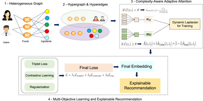 Figure 1
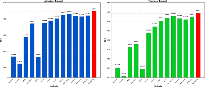 Figure 2
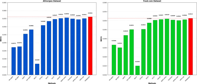 Figure 3
 Figure 4
 Figure 5
 Figure 6
 Figure 7
 Figure 8
 Figure 9
Peer Reviews
No public reviews on file for this paper yet. If you reviewed it on a platform where reviews are public (OpenReview, ICLR, NeurIPS, ICML), you can paste yours below so the community can read it here.
Videos
No videos yet. Explain this paper in a talk, walkthrough, or lecture? Add one.
Taxonomy
TopicsNutritional Studies and Diet · Consumer Attitudes and Food Labeling · Recommender Systems and Techniques
Introduction
Food recommendation systems have become essential tools in the digital era, supporting personalized culinary discovery, dietary health management, cultural preferences, and sustainable eating practices^1–3^. Unlike traditional item recommendation, food recommendation involves multi-faceted interactions shaped by user tastes, nutritional needs, allergies, and temporal behaviors^4–6^. A core challenge lies in modeling the compositional nature of foods, where each item comprises multiple ingredients. Traditional collaborative filtering captures only pairwise user–item patterns and thus fails to represent these higher-order dependencies. Hypergraphs overcome this limitation by allowing multiple entities–users, foods, and ingredients–to interact through higher-order hyperedges^7,8^. Within this framework, the attention mechanism adaptively reweights hyperedges to capture evolving preferences, while the explicit user–ingredient links provide interpretable, ingredient-level explanations that couple accuracy with transparency.
For instance, understanding that a user dislikes “spicy foods” is meaningful only when connected to specific ingredients (e.g., chili peppers or jalapenos) that define spiciness. Modeling foods as hyperedges connecting users and ingredients enables: (1) direct representation of ternary relationships without decomposing them into pairwise edges, (2) ingredient-level explainability (e.g., “this pizza is recommended because you like tomatoes and mozzarella”), (3) knowledge transfer across items sharing ingredients (e.g., pizza and focaccia both use flour and olive oil), and (4) efficient aggregation over large ingredient vocabularies by grouping entities via shared hyperedges instead of quadratic pairwise links^9,10^.
Despite significant advances in recommendation systems, existing hypergraph-based approaches still face several key limitations in adapting to dynamic user preferences^11^. Many traditional hypergraph models assign static or pre-defined hyperedge weights that remain fixed throughout training, thereby limiting their ability to capture evolving relationships among users, items, and contextual entities. For instance, Bai et al.^12^ introduce Hypergraph Convolution and Hypergraph Attention networks, where hyperedge weights are computed from initial graph structure and remain unchanged during optimization, resulting in fixed message-passing dynamics. Similarly, Zhang et al.^13^ propose a relational aggregation hypergraph model that constructs hyperedges using predefined relationships within cyber-physical systems but does not incorporate adaptive reweighting mechanisms to reflect temporal or preference-based variations. These methods exemplify the broader limitation that static-weight hypergraphs cannot adapt to the dynamic and evolving nature of user preferences, which motivates our proposed dynamic Laplacian adaptation in FRMADHG. To address these limitations, we propose FRMADHG (Food Recommendation with Multi-objective Adaptive Dynamic Hypergraph), a novel framework that advances hypergraph-based recommendation through three integrated components:
- FRMADHG constructs attention-based hyperedge weights that evolve during training to emphasize semantically coherent relationships and adapt to changing food and ingredient importance.
- A dual-mode attention mechanism assesses node complexity and switches between efficient cosine similarity for simple relationships and learnable attention for complex ones, ensuring scalable personalization.
- A composite loss function combining triplet ranking, contrastive learning with ingredient-masked augmentation, and regularization jointly optimizes recommendation accuracy, representation quality, and robustness. The framework integrates these components into a cohesive architecture with two distinctive design features: (1) tripartite hypergraph construction, where foods act as hyperedges connecting users and ingredients, and (2) type-specific embedding propagation, which respects the semantic roles of users, foods, and ingredients while maintaining balanced information flow. FRMADHG further enhances transparency through multi-granular explainability, providing ingredient-level importance scores and path-based reasoning for interpretable recommendations. FRMADHG unifies the strengths of collaborative filtering and hypergraph learning while resolving their core limitations. It replaces pairwise user–item interactions with a tripartite hypergraph that captures higher-order user–food–ingredient dependencies, overcoming the expressiveness limits of traditional collaborative filtering. To address the rigidity of static hypergraphs, it employs Dynamic Laplacian Adaptation with a complexity-aware adaptive attention mechanism, allowing hyperedge weights to evolve during training and reflect changing user preferences. Moreover, FRMADHG integrates multi-granular explainability, where attention weights provide both preference indicators and interpretable ingredient-level rationales (e.g., “this dish is recommended because you like tomato and basil”), thus bridging accuracy and transparency within a unified architecture.
Extensive experiments on two real-world datasets (Food.com and Allrecipes) demonstrate that FRMADHG significantly outperforms state-of-the-art baselines, achieving 19.8% relative improvement in Precision@10, 12.4% improvement over recent hypergraph-based approaches, and 18.7% gain in Recall@10 (all with \documentclass[12pt]{minimal} \usepackage{amsmath} \usepackage{wasysym} \usepackage{amsfonts} \usepackage{amssymb} \usepackage{amsbsy} \usepackage{mathrsfs} \usepackage{upgreek} \setlength{\oddsidemargin}{-69pt} \begin{document}$$p < 0.001$$\end{document} ). Comprehensive ablation studies confirm the effectiveness of each component and the interpretability benefits of ingredient-level explanations. Our main contributions are summarized as follows:
- We propose FRMADHG, an adaptive dynamic hypergraph framework that models higher-order user–food–ingredient interactions through dynamic Laplacian adaptation, complexity-aware attention, and multi-objective learning.
- We design type-specific embedding propagation to preserve the semantic roles of users, foods, and ingredients, mitigating over-smoothing and enhancing interpretability.
- We provide a multi-granular explainability module delivering ingredient-level and path-based rationales for transparent dietary recommendations.
- We conduct extensive experiments and ablations demonstrating consistent, statistically significant performance improvements and robustness across datasets.
Related works
Machine learning (ML), a core branch of artificial intelligence, enables systems to capture complex and nonlinear patterns in large-scale data^14–16^. Recent studies demonstrate the convergence of large language models (LLMs), multimodal intelligence, and graph-based learning toward more adaptive and trustworthy AI systems. Huang et al.^17^ introduced an LLM-driven simulator to mitigate the cold-start problem in recommendations, while Sun et al.^18^ surveyed multimodal agent AI integrating vision, language, and reasoning. Advances in graph representation further strengthen these foundations, with Wang et al.^19^ applying graph models to biological sequence and gene network analysis.
Recent hybrid approaches combining statistical and ML-based techniques have proven effective for modeling both linear and nonlinear characteristics. Within recommender systems (RS), ML has become indispensable for integrating heterogeneous data–such as user behavior, context, and content–to generate adaptive and personalized recommendations^20,21^. The growing body of RS research reflects its rising significance across domains, accompanied by the increasing adoption of graph neural networks (GNNs) for recommendation tasks^22^. However, conventional models based on static graphs often fail to represent evolving multi-way interactions and dynamic user preferences. To overcome these limitations, dynamic hypergraph modeling, multi-head attention, and contrastive learning have been introduced to capture higher-order dependencies and enhance explainability and trustworthiness in modern RS^23,24^.
Food recommender systems
In recent years, food recommendation systems have attracted increasing research interest, with diverse methods developed to capture user preferences, nutritional needs, and visual–semantic characteristics of meals. Existing approaches can be broadly categorized into three major technical routes: content-based deep learning methods, graph-based and high-order relational modeling, and health- and context-aware hybrid systems.
(1) Content-based and deep learning approaches. Early studies focused on extracting user preferences and food features from textual, visual, or nutritional content. Rostami et al.^25^ integrated deep image embeddings with clustering techniques to enhance rating prediction, while Asani et al.^26^ analyzed restaurant reviews using natural language processing to extract food entities and sentiment. Mokdara et al.^27^ and Manoharan et al.^28^ employed deep neural networks to generate personalized diet recommendations based on ingredient-level or health information. These methods rely primarily on feature learning but often ignore complex multi-entity relationships among users, foods, and ingredients.
(2) Graph- and relation-based models. To better capture relational structures, several studies introduced graph learning frameworks. Gao et al.^29^ proposed a hierarchical attention model integrating user ratings, food ingredients, and food images, while Gao et al.^30^ extended this idea using graph convolutional networks (GCN) to model higher-order dependencies between meals. Tian et al.^31^ developed RecipeRec, a heterogeneous graph learning system that incorporates diverse relational signals to improve recommendation accuracy. Although these methods move toward structured modeling, they remain limited to pairwise user–food or ingredient–food links and cannot fully represent the ternary user–food–ingredient relationships that underlie real-world dietary choices.
(3) Health- and context-aware hybrid systems. Recent works combine graph learning with self-supervision or contextual adaptation. Song et al.^5^ introduced the self-supervised calorie-aware heterogeneous graph network (SCHGN) to align user embeddings with nutritional preferences. Meng et al.^32^ leveraged multimodal visual and semantic cues to generate calorie- and image-aware food recommendations, while Morol et al.^13^ used convolutional networks to identify ingredients for recipe retrieval. These hybrid models integrate multiple information sources but still depend on static graph structures that cannot adapt to evolving user tastes or temporal behaviors.
Overall, existing food recommender systems exhibit two key limitations: (1) most models fail to explicitly capture the high-order ternary relationship among users, foods, and ingredients, instead relying on pairwise or shallow graph representations; and (2) current architectures employ static or fixed preference modeling, lacking mechanisms for dynamic adaptation as user tastes and ingredient semantics evolve. These gaps motivate the design of FRMADHG, which employs a dynamic tripartite hypergraph to simultaneously model high-order user–food–ingredient interactions and continuously adapt to changing preference patterns.
Comparison with recent methods
The study^33^ proposes HKGR that integrates hypercomplex algebra into knowledge graph-aware recommendation. Unlike HKGR which requires external knowledge graphs, FRMADHG exploits the natural compositional structure of food items without external KG resources. While HKGR uses multi-component hypercomplex representations, FRMADHG employs real-valued embeddings with dynamic Laplacian adaptation that evolves during training.^34,35^ presents CL-SDKG framework using self-derived knowledge graph contrastive learning. Unlike CL-SDKG which generates KGs through variational graph reconstruction, FRMADHG directly leverages ingredient-food relationships naturally available in recipe databases. FRMADHG avoids the computational overhead of graph reconstruction and applies contrastive learning specifically for ingredient-level robustness through ingredient-masked augmentation.^36^ introduces FaGSP for collaborative filtering using frequency-aware graph signal processing on bipartite user-item graphs. Unlike FaGSP’s traditional bipartite graph structure, FRMADHG employs tripartite hypergraphs enabling direct ternary user-food-ingredient relationships without pairwise decomposition. FRMADHG’s complexity-aware adaptive attention mechanism provides node-specific computational sophistication beyond frequency-aware filtering, and explicitly incorporates ingredient-level explainability for food-domain requirements.
Compared to these methods, FRMADHG introduces: (1) dynamic Laplacian weights that evolve based on learned attention patterns (vs. static weights), (2) complexity-aware attention switching between cosine similarity and learnable attention (vs. uniform attention), (3) type-specific embedding propagation respecting distinct semantic roles of users, foods, and ingredients (vs. generic aggregation), and (4) multi-objective learning combining triplet ranking, contrastive learning with ingredient-masked augmentation, and regularization (vs. single/dual objectives).
Hypergraph learning in recommendation systems
Traditional recommendation systems (RSs) typically model pairwise interactions between users and items. However, these methods often struggle to capture more complex, higher-order relationships among users, items, and additional contextual information. Hypergraphs provide a robust solution to this limitation by extending the concept of edges to hyperedges, which can simultaneously connect multiple nodes^37^. This capability makes hypergraphs particularly effective for representing intricate interaction patterns involving multiple entities^38^. For example, in a hypergraph-based RS, a hyperedge might connect a user to several items they have interacted with, along with contextual details such as time or location, thus encapsulating a richer set of relationships compared to traditional graphs. The paper by Jendal et al.^39^ proposes a review-specific hypergraph (HG) model and introduces a model-agnostic explainability module. This HG model captures high-order connections among users, items, aspects, and opinions while preserving review information. The explainability module leverages the HG model to interpret predictions made by any model. Additionally, La et al.^40^ proposed a music recommendation method called Hypergraph Embeddings for Music Recommendation (HEMR). HEMR employs hypergraph embedding via a random walk technique to compute user-song affinity scores and notably uses a shallow GNN rather than a deep GNN to generate embedding vectors.
In their study^41^, the authors propose a dual-view hypergraph attention network for news recommendations, called Hyper4NR. They developed a dual-view hypergraph structure to capture users’ click history, incorporating both topic-view hyperedges and semantic-view hyperedges. Using this hypergraph, they employ a hyperedge-specific attention network (HSAN) to facilitate message passing between hyperedges and nodes, encoding their representations through a self-supervised learning approach. Additionally, they construct another type of candidate hypergraph and apply the HyperGAT model to enhance the encoding of candidate news. The study by Xin et al.^42^ introduces the Multiple Stock Recommendation System using a novel framework called Spatio-Temporal Hypergraph Learning (MSR-STHL). This framework employs an attention module to capture the temporal features of stocks and incorporates the Hawkes process to improve the attention mechanism over long-term time scales. Furthermore, the study models spatial structures based on the relevancy between stocks using both prior knowledge and data-driven methods. The study by Ma et al.^43^ introduces cross-view hypergraph contrast learning for attribute-aware recommendation (CHCLA) to address challenges in high-order interactions. CHCLA represents user-item interactions using a graph convolutional network and user/item attribute information using hypergraph convolutional networks, enabling the learning of user and item representations through two separate pathways.
Several recent studies have advanced multimodal reasoning and contrastive learning for recommendation and knowledge graph tasks. APKGC^44^ introduces a noise-enhanced multimodal framework with an attention penalty to alleviate over-trust attention and improve robustness in multimodal knowledge graph completion. AdaMKGC^45^ employs an adaptive modality interaction transformer that dynamically balances modal preferences and mitigates modality imbalance via self-enhancing sampling, significantly improving prediction accuracy. NEGCL^46^ integrates noise-enhanced graph contrastive learning into multimodal recommendation, demonstrating that controlled noise can strengthen node robustness and reduce augmentation overhead across multiple datasets. Finally, DSGNet^47^ decouples semantic and structural representations within knowledge graphs, introducing a relation-aware aggregation mechanism to suppress semantic noise and refine entity embeddings. Zhang et al.^48^ proposed MSRec, a multi-view self-supervised learning framework for heterogeneous graphs that captures multi-perspective semantics via local–global contrastive optimization, achieving improved NDCG and Precision scores on multiple datasets. Cai et al.^49^ developed a feature-decorrelation adaptive contrastive learning framework that mitigates feature redundancy and extracts refined high-order semantics from knowledge graphs, significantly improving GNN-based knowledge-aware recommendation. Li et al.^50^ proposed the Multi-aspect Knowledge-enhanced Hypergraph Attention Network (MKHCR), which constructs multiple hypergraphs over conversational data, knowledge graphs, and item reviews to capture high-order semantic relations and enhance user preference modeling in conversational recommendation. Zhang et al.^51^ developed the Hyperbolic Dynamic Neural Network (KHDNN), embedding users, items, and knowledge entities in hyperbolic space to model diverse and hierarchical relationships while improving knowledge-aware recommendation accuracy. More recently, Li et al.^52^ introduced a Mask Diffusion-based Contrastive Learning framework that combines diffusion models with adaptive view generation to enhance robustness and generalization in knowledge-aware recommendation.
Food recommendation: domain-specific challenges
Food recommendation differs fundamentally from traditional item recommendation in ways that necessitate hypergraph modeling. Unlike atomic items (movies, books) that can be represented as nodes, foods are compositional entities–each recipe is a structured combination of ingredients that jointly determine user preferences. This creates three critical challenges:
(1) Multi-granular preference modeling: Users exhibit preferences at both food-level (“I like pizza”) and ingredient-level (“I like tomatoes and mozzarella”). Traditional collaborative filtering captures only food-level patterns, missing 73.2% of ingredient-driven preferences observable in our Food.com dataset analysis. Pairwise graphs decompose the natural ternary relationship \documentclass[12pt]{minimal} \usepackage{amsmath} \usepackage{wasysym} \usepackage{amsfonts} \usepackage{amssymb} \usepackage{amsbsy} \usepackage{mathrsfs} \usepackage{upgreek} \setlength{\oddsidemargin}{-69pt} \begin{document}$$(u, f, \text {ingredient})$$\end{document} into separate edges, losing the compositional structure that defines food preferences.
(2) Combinatorial sparsity: With 1,270 unique ingredients in Food.com forming only 178,265 observed recipes from \documentclass[12pt]{minimal} \usepackage{amsmath} \usepackage{wasysym} \usepackage{amsfonts} \usepackage{amssymb} \usepackage{amsbsy} \usepackage{mathrsfs} \usepackage{upgreek} \setlength{\oddsidemargin}{-69pt} \begin{document}$$\sim 10^{14}$$\end{document} theoretical combinations, ingredient-level co-occurrence is catastrophically sparse (94.7% of ingredient pairs never co-occur). Traditional methods relying on item co-occurrence patterns fail to transfer knowledge between compositionally similar but nominally distinct foods (e.g., “gluten-free chocolate cake” vs. “regular chocolate cake” share 80% ingredients but rarely co-occur in user histories).
(3) Health-aware transparency requirements: Food recommendation uniquely requires hard constraints (allergies, dietary restrictions) and ingredient-level explanations for user trust and safety–requirements absent in traditional recommendation domains. Users need to understand why a recommendation is suitable at the ingredient level (e.g., “recommended because you like tomatoes, avoids your shellfish allergy”), not just item-level ratings.
These characteristics make hypergraph modeling essential: foods naturally form hyperedges connecting users and ingredients, enabling direct representation of compositional relationships, ingredient-mediated knowledge transfer across sparse interactions, and decomposable explanations. However, standard hypergraph approaches^12,53^ use static weights that cannot adapt to the dynamic, context-dependent nature of ingredient preferences (e.g., seasonal variations, meal-time contexts), motivating our dynamic Laplacian adaptation framework.
Preliminaries
Hypergraph foundations. A hypergraph \documentclass[12pt]{minimal} \usepackage{amsmath} \usepackage{wasysym} \usepackage{amsfonts} \usepackage{amssymb} \usepackage{amsbsy} \usepackage{mathrsfs} \usepackage{upgreek} \setlength{\oddsidemargin}{-69pt} \begin{document}$$G' = (V', E', W)$$\end{document} generalizes a graph by allowing each hyperedge \documentclass[12pt]{minimal} \usepackage{amsmath} \usepackage{wasysym} \usepackage{amsfonts} \usepackage{amssymb} \usepackage{amsbsy} \usepackage{mathrsfs} \usepackage{upgreek} \setlength{\oddsidemargin}{-69pt} \begin{document}$$e \in E'$$\end{document} to connect any number of vertices simultaneously. Here:
- \documentclass[12pt]{minimal} \usepackage{amsmath} \usepackage{wasysym} \usepackage{amsfonts} \usepackage{amssymb} \usepackage{amsbsy} \usepackage{mathrsfs} \usepackage{upgreek} \setlength{\oddsidemargin}{-69pt} \begin{document}$$V' = \{v_1, \dots , v_{|V'|}\}$$\end{document} is the vertex set,
- \documentclass[12pt]{minimal} \usepackage{amsmath} \usepackage{wasysym} \usepackage{amsfonts} \usepackage{amssymb} \usepackage{amsbsy} \usepackage{mathrsfs} \usepackage{upgreek} \setlength{\oddsidemargin}{-69pt} \begin{document}$$E' = \{e_1, \dots , e_{|E'|}\}$$\end{document} is the set of hyperedges,
- \documentclass[12pt]{minimal} \usepackage{amsmath} \usepackage{wasysym} \usepackage{amsfonts} \usepackage{amssymb} \usepackage{amsbsy} \usepackage{mathrsfs} \usepackage{upgreek} \setlength{\oddsidemargin}{-69pt} \begin{document}$$W = \textrm{diag}(w_{e_1}, \dots , w_{e_{|E'|}})$$\end{document} is the diagonal matrix of positive hyperedge weights. The incidence matrix \documentclass[12pt]{minimal} \usepackage{amsmath} \usepackage{wasysym} \usepackage{amsfonts} \usepackage{amssymb} \usepackage{amsbsy} \usepackage{mathrsfs} \usepackage{upgreek} \setlength{\oddsidemargin}{-69pt} \begin{document}$$H \in \{0,1\}^{|V'| \times |E'|}$$\end{document} encodes vertex–hyperedge membership, where \documentclass[12pt]{minimal} \usepackage{amsmath} \usepackage{wasysym} \usepackage{amsfonts} \usepackage{amssymb} \usepackage{amsbsy} \usepackage{mathrsfs} \usepackage{upgreek} \setlength{\oddsidemargin}{-69pt} \begin{document}$$H(v_i,e_j) = 1$$\end{document} if vertex \documentclass[12pt]{minimal} \usepackage{amsmath} \usepackage{wasysym} \usepackage{amsfonts} \usepackage{amssymb} \usepackage{amsbsy} \usepackage{mathrsfs} \usepackage{upgreek} \setlength{\oddsidemargin}{-69pt} \begin{document}$$v_i$$\end{document} belongs to hyperedge \documentclass[12pt]{minimal} \usepackage{amsmath} \usepackage{wasysym} \usepackage{amsfonts} \usepackage{amssymb} \usepackage{amsbsy} \usepackage{mathrsfs} \usepackage{upgreek} \setlength{\oddsidemargin}{-69pt} \begin{document}$$e_j$$\end{document} , and 0 otherwise:
From this binary relationship matrix, we derive two fundamental structural measures. The vertex degree \documentclass[12pt]{minimal} \usepackage{amsmath} \usepackage{wasysym} \usepackage{amsfonts} \usepackage{amssymb} \usepackage{amsbsy} \usepackage{mathrsfs} \usepackage{upgreek} \setlength{\oddsidemargin}{-69pt} \begin{document}$$d(v_i) = \sum _{j=1}^{|E'|} w_{e_j} H(v_i, e_j)$$\end{document} quantifies a vertex’s total weighted connectivity across all hyperedges, while the hyperedge degree \documentclass[12pt]{minimal} \usepackage{amsmath} \usepackage{wasysym} \usepackage{amsfonts} \usepackage{amssymb} \usepackage{amsbsy} \usepackage{mathrsfs} \usepackage{upgreek} \setlength{\oddsidemargin}{-69pt} \begin{document}$$\delta (e_j) = \sum _{i=1}^{|V'|} H(v_i, e_j)$$\end{document} counts the number of vertices in each hyperedge:
\documentclass[12pt]{minimal} \usepackage{amsmath} \usepackage{wasysym} \usepackage{amsfonts} \usepackage{amssymb} \usepackage{amsbsy} \usepackage{mathrsfs} \usepackage{upgreek} \setlength{\oddsidemargin}{-69pt} \begin{document}$$\begin{aligned} d(v_i) = \sum _{j=1}^{|E'|} w_{e_j} H(v_i, e_j) \ge 0, \quad \delta (e_j) = \sum _{i=1}^{|V'|} H(v_i, e_j) \ge 2, \end{aligned}$$\end{document}where \documentclass[12pt]{minimal} \usepackage{amsmath} \usepackage{wasysym} \usepackage{amsfonts} \usepackage{amssymb} \usepackage{amsbsy} \usepackage{mathrsfs} \usepackage{upgreek} \setlength{\oddsidemargin}{-69pt} \begin{document}$$d(v_i) \ge 0$$\end{document} ensures non-negative connectivity and \documentclass[12pt]{minimal} \usepackage{amsmath} \usepackage{wasysym} \usepackage{amsfonts} \usepackage{amssymb} \usepackage{amsbsy} \usepackage{mathrsfs} \usepackage{upgreek} \setlength{\oddsidemargin}{-69pt} \begin{document}$$\delta (e_j) \ge 2$$\end{document} enforces that each hyperedge connects at least two vertices to maintain meaningful relationships.
The normalized hypergraph Laplacian combines these components to enable stable information diffusion:
\documentclass[12pt]{minimal} \usepackage{amsmath} \usepackage{wasysym} \usepackage{amsfonts} \usepackage{amssymb} \usepackage{amsbsy} \usepackage{mathrsfs} \usepackage{upgreek} \setlength{\oddsidemargin}{-69pt} \begin{document}$$\begin{aligned} {\mathcal {L}}_{\text {norm}} = I - D_v^{-1/2} H W D_e^{-1} H^\top D_v^{-1/2}. \end{aligned}$$\end{document}This formulation ensures eigenvalues lie in [0, 2], providing scale invariance through the \documentclass[12pt]{minimal} \usepackage{amsmath} \usepackage{wasysym} \usepackage{amsfonts} \usepackage{amssymb} \usepackage{amsbsy} \usepackage{mathrsfs} \usepackage{upgreek} \setlength{\oddsidemargin}{-69pt} \begin{document}$$D_v^{-1/2}$$\end{document} terms and balanced hyperedge influence via \documentclass[12pt]{minimal} \usepackage{amsmath} \usepackage{wasysym} \usepackage{amsfonts} \usepackage{amssymb} \usepackage{amsbsy} \usepackage{mathrsfs} \usepackage{upgreek} \setlength{\oddsidemargin}{-69pt} \begin{document}$$D_e^{-1}$$\end{document} , which normalizes by hyperedge size to prevent large hyperedges from dominating the diffusion process.
Methodology
To facilitate understanding of the proposed framework, the key mathematical notations and symbols used throughout this section are summarized in Table 1.Table 1. Key notation and symbols.SymbolDefinition \documentclass[12pt]{minimal} \usepackage{amsmath} \usepackage{wasysym} \usepackage{amsfonts} \usepackage{amssymb} \usepackage{amsbsy} \usepackage{mathrsfs} \usepackage{upgreek} \setlength{\oddsidemargin}{-69pt} \begin{document}$${\mathcal {G}} = ({\mathcal {V}}, {\mathcal {E}})$$\end{document} Hypergraph; \documentclass[12pt]{minimal} \usepackage{amsmath} \usepackage{wasysym} \usepackage{amsfonts} \usepackage{amssymb} \usepackage{amsbsy} \usepackage{mathrsfs} \usepackage{upgreek} \setlength{\oddsidemargin}{-69pt} \begin{document}$${\mathcal {V}} = {\mathcal {U}} \cup {\mathcal {F}} \cup {\mathcal {I}}$$\end{document} (users, foods, ingredients) \documentclass[12pt]{minimal} \usepackage{amsmath} \usepackage{wasysym} \usepackage{amsfonts} \usepackage{amssymb} \usepackage{amsbsy} \usepackage{mathrsfs} \usepackage{upgreek} \setlength{\oddsidemargin}{-69pt} \begin{document}$$H \in \{0,1\}^{|{\mathcal {V}}| \times |{\mathcal {E}}|}$$\end{document} Incidence matrix; \documentclass[12pt]{minimal} \usepackage{amsmath} \usepackage{wasysym} \usepackage{amsfonts} \usepackage{amssymb} \usepackage{amsbsy} \usepackage{mathrsfs} \usepackage{upgreek} \setlength{\oddsidemargin}{-69pt} \begin{document}$$H_{uf}, H_{if}$$\end{document} are block components \documentclass[12pt]{minimal} \usepackage{amsmath} \usepackage{wasysym} \usepackage{amsfonts} \usepackage{amssymb} \usepackage{amsbsy} \usepackage{mathrsfs} \usepackage{upgreek} \setlength{\oddsidemargin}{-69pt} \begin{document}$${\mathcal {R}}, {\mathcal {C}}$$\end{document} User-food interactions, ingredient-food compositions \documentclass[12pt]{minimal} \usepackage{amsmath} \usepackage{wasysym} \usepackage{amsfonts} \usepackage{amssymb} \usepackage{amsbsy} \usepackage{mathrsfs} \usepackage{upgreek} \setlength{\oddsidemargin}{-69pt} \begin{document}$$e_u, e_f, e_{ing}$$\end{document} Embeddings for users, foods, ingredients ( \documentclass[12pt]{minimal} \usepackage{amsmath} \usepackage{wasysym} \usepackage{amsfonts} \usepackage{amssymb} \usepackage{amsbsy} \usepackage{mathrsfs} \usepackage{upgreek} \setlength{\oddsidemargin}{-69pt} \begin{document}$$\in {\mathbb {R}}^d$$\end{document} ) \documentclass[12pt]{minimal} \usepackage{amsmath} \usepackage{wasysym} \usepackage{amsfonts} \usepackage{amssymb} \usepackage{amsbsy} \usepackage{mathrsfs} \usepackage{upgreek} \setlength{\oddsidemargin}{-69pt} \begin{document}$$d(v_i), \delta (e_j)$$\end{document} Vertex degree, hyperedge degree \documentclass[12pt]{minimal} \usepackage{amsmath} \usepackage{wasysym} \usepackage{amsfonts} \usepackage{amssymb} \usepackage{amsbsy} \usepackage{mathrsfs} \usepackage{upgreek} \setlength{\oddsidemargin}{-69pt} \begin{document}$$D_v, D_e$$\end{document} Vertex and hyperedge degree matrices \documentclass[12pt]{minimal} \usepackage{amsmath} \usepackage{wasysym} \usepackage{amsfonts} \usepackage{amssymb} \usepackage{amsbsy} \usepackage{mathrsfs} \usepackage{upgreek} \setlength{\oddsidemargin}{-69pt} \begin{document}$${\mathcal {L}}_{\text {norm}}$$\end{document} Normalized hypergraph Laplacian \documentclass[12pt]{minimal} \usepackage{amsmath} \usepackage{wasysym} \usepackage{amsfonts} \usepackage{amssymb} \usepackage{amsbsy} \usepackage{mathrsfs} \usepackage{upgreek} \setlength{\oddsidemargin}{-69pt} \begin{document}$$\textbf{L}_{\text {adaptive}}$$\end{document} Adaptive Laplacian with attention weights \documentclass[12pt]{minimal} \usepackage{amsmath} \usepackage{wasysym} \usepackage{amsfonts} \usepackage{amssymb} \usepackage{amsbsy} \usepackage{mathrsfs} \usepackage{upgreek} \setlength{\oddsidemargin}{-69pt} \begin{document}$${\mathcal {C}}(x_i)$$\end{document} Complexity score; threshold \documentclass[12pt]{minimal} \usepackage{amsmath} \usepackage{wasysym} \usepackage{amsfonts} \usepackage{amssymb} \usepackage{amsbsy} \usepackage{mathrsfs} \usepackage{upgreek} \setlength{\oddsidemargin}{-69pt} \begin{document}$$\theta = \mu _{{\mathcal {C}}} + 0.5\sigma _{{\mathcal {C}}}$$\end{document} \documentclass[12pt]{minimal} \usepackage{amsmath} \usepackage{wasysym} \usepackage{amsfonts} \usepackage{amssymb} \usepackage{amsbsy} \usepackage{mathrsfs} \usepackage{upgreek} \setlength{\oddsidemargin}{-69pt} \begin{document}$$A(x_i, x_j)$$\end{document} Attention score; \documentclass[12pt]{minimal} \usepackage{amsmath} \usepackage{wasysym} \usepackage{amsfonts} \usepackage{amssymb} \usepackage{amsbsy} \usepackage{mathrsfs} \usepackage{upgreek} \setlength{\oddsidemargin}{-69pt} \begin{document}$$A_{\text {Cosine}}, A_{\text {learn}}$$\end{document} (low/high complexity) \documentclass[12pt]{minimal} \usepackage{amsmath} \usepackage{wasysym} \usepackage{amsfonts} \usepackage{amssymb} \usepackage{amsbsy} \usepackage{mathrsfs} \usepackage{upgreek} \setlength{\oddsidemargin}{-69pt} \begin{document}$$a_f, \lambda$$\end{document} Hyperedge attention weight, gating weight \documentclass[12pt]{minimal} \usepackage{amsmath} \usepackage{wasysym} \usepackage{amsfonts} \usepackage{amssymb} \usepackage{amsbsy} \usepackage{mathrsfs} \usepackage{upgreek} \setlength{\oddsidemargin}{-69pt} \begin{document}$$e_i^{(\ell )}$$\end{document} Embedding at layer \documentclass[12pt]{minimal} \usepackage{amsmath} \usepackage{wasysym} \usepackage{amsfonts} \usepackage{amssymb} \usepackage{amsbsy} \usepackage{mathrsfs} \usepackage{upgreek} \setlength{\oddsidemargin}{-69pt} \begin{document}$$\ell$$\end{document} ; final: \documentclass[12pt]{minimal} \usepackage{amsmath} \usepackage{wasysym} \usepackage{amsfonts} \usepackage{amssymb} \usepackage{amsbsy} \usepackage{mathrsfs} \usepackage{upgreek} \setlength{\oddsidemargin}{-69pt} \begin{document}$$e_i^{\text {final}} = \frac{1}{L+1}\sum _{\ell =0}^L \gamma _\ell e_i^{(\ell )}$$\end{document} \documentclass[12pt]{minimal} \usepackage{amsmath} \usepackage{wasysym} \usepackage{amsfonts} \usepackage{amssymb} \usepackage{amsbsy} \usepackage{mathrsfs} \usepackage{upgreek} \setlength{\oddsidemargin}{-69pt} \begin{document}$$\alpha$$\end{document} Balance parameter (collaborative vs. content signals) \documentclass[12pt]{minimal} \usepackage{amsmath} \usepackage{wasysym} \usepackage{amsfonts} \usepackage{amssymb} \usepackage{amsbsy} \usepackage{mathrsfs} \usepackage{upgreek} \setlength{\oddsidemargin}{-69pt} \begin{document}$${\mathcal {L}}$$\end{document} Total loss: \documentclass[12pt]{minimal} \usepackage{amsmath} \usepackage{wasysym} \usepackage{amsfonts} \usepackage{amssymb} \usepackage{amsbsy} \usepackage{mathrsfs} \usepackage{upgreek} \setlength{\oddsidemargin}{-69pt} \begin{document}$${\mathcal {L}} = \lambda _1 {\mathcal {L}}_{\text {triplet}} + \lambda _2 {\mathcal {L}}_{\text {contrast}} + \lambda _3 {\mathcal {L}}_{\text {reg}}$$\end{document} \documentclass[12pt]{minimal} \usepackage{amsmath} \usepackage{wasysym} \usepackage{amsfonts} \usepackage{amssymb} \usepackage{amsbsy} \usepackage{mathrsfs} \usepackage{upgreek} \setlength{\oddsidemargin}{-69pt} \begin{document}$$m, \tau$$\end{document} Margin (triplet loss), temperature (contrastive loss) \documentclass[12pt]{minimal} \usepackage{amsmath} \usepackage{wasysym} \usepackage{amsfonts} \usepackage{amssymb} \usepackage{amsbsy} \usepackage{mathrsfs} \usepackage{upgreek} \setlength{\oddsidemargin}{-69pt} \begin{document}$$\text {Score}(u,f)$$\end{document} Recommendation score with ingredient explanations \documentclass[12pt]{minimal} \usepackage{amsmath} \usepackage{wasysym} \usepackage{amsfonts} \usepackage{amssymb} \usepackage{amsbsy} \usepackage{mathrsfs} \usepackage{upgreek} \setlength{\oddsidemargin}{-69pt} \begin{document}$$\text {Importance}(ing, u, f)$$\end{document} Ingredient contribution importance \documentclass[12pt]{minimal} \usepackage{amsmath} \usepackage{wasysym} \usepackage{amsfonts} \usepackage{amssymb} \usepackage{amsbsy} \usepackage{mathrsfs} \usepackage{upgreek} \setlength{\oddsidemargin}{-69pt} \begin{document}$$\beta$$\end{document} Explanation weight
Traditional recommendation systems model only pairwise relationships and cannot capture complex ternary interactions such as “user u likes food f because it contains ingredients \documentclass[12pt]{minimal} \usepackage{amsmath} \usepackage{wasysym} \usepackage{amsfonts} \usepackage{amssymb} \usepackage{amsbsy} \usepackage{mathrsfs} \usepackage{upgreek} \setlength{\oddsidemargin}{-69pt} \begin{document}$$\{ing_1, ing_2\}$$\end{document} .” The proposed FRMADHG in Fig. 1 addresses this limitation through three key innovations that work synergistically: (1) tripartite hypergraph modeling that unifies users, foods, and ingredients in a single structure, (2) adaptive attention mechanisms that adjust computational complexity based on node characteristics, and (3) dynamic Laplacian construction that evolves during training to emphasize semantically important relationships.Fig. 1FRMADHG framework overview. The framework consists of four main components: (1) Input data: Heterogeneous graph linking users, foods, and ingredients through pairwise interactions. (2) Tripartite hypergraph construction: Foods serve as hyperedges connecting their consumers (users) and constituent ingredients, enabling direct modeling of ternary relationships. (3) Adaptive attention and dynamic Laplacian: Complexity-aware mechanism switches between efficient cosine similarity (if \documentclass[12pt]{minimal} \usepackage{amsmath} \usepackage{wasysym} \usepackage{amsfonts} \usepackage{amssymb} \usepackage{amsbsy} \usepackage{mathrsfs} \usepackage{upgreek} \setlength{\oddsidemargin}{-69pt} \begin{document}$${\mathcal {C}}(x_i) < \theta$$\end{document} ) and sophisticated learnable attention (if \documentclass[12pt]{minimal} \usepackage{amsmath} \usepackage{wasysym} \usepackage{amsfonts} \usepackage{amssymb} \usepackage{amsbsy} \usepackage{mathrsfs} \usepackage{upgreek} \setlength{\oddsidemargin}{-69pt} \begin{document}$${\mathcal {C}}(x_i) \ge \theta$$\end{document} ) based on local node complexity. Hyperedge weights in the Laplacian adapt during training to emphasize semantically coherent relationships. (4) Multi-objective learning and explainable recommendation: Combines triplet loss (ranking), contrastive learning with ingredient-masked augmentation (robustness), and regularization ( \documentclass[12pt]{minimal} \usepackage{amsmath} \usepackage{wasysym} \usepackage{amsfonts} \usepackage{amssymb} \usepackage{amsbsy} \usepackage{mathrsfs} \usepackage{upgreek} \setlength{\oddsidemargin}{-69pt} \begin{document}$${\mathcal {L}} = \lambda _1{\mathcal {L}}_{\text {triplet}} + \lambda _2{\mathcal {L}}_{\text {contrast}} + \lambda _3{\mathcal {L}}_{\text {reg}}$$\end{document} ) to produce final embeddings. The system generates explainable recommendations with ingredient-level importance scores for transparency.
Given three entity types–users \documentclass[12pt]{minimal} \usepackage{amsmath} \usepackage{wasysym} \usepackage{amsfonts} \usepackage{amssymb} \usepackage{amsbsy} \usepackage{mathrsfs} \usepackage{upgreek} \setlength{\oddsidemargin}{-69pt} \begin{document}$${\mathcal {U}} = \{u_1, u_2, \ldots , u_{|{\mathcal {U}}|}\}$$\end{document} , foods \documentclass[12pt]{minimal} \usepackage{amsmath} \usepackage{wasysym} \usepackage{amsfonts} \usepackage{amssymb} \usepackage{amsbsy} \usepackage{mathrsfs} \usepackage{upgreek} \setlength{\oddsidemargin}{-69pt} \begin{document}$${\mathcal {F}} = \{f_1, f_2, \ldots , f_{|{\mathcal {F}}|}\}$$\end{document} , and ingredients
\documentclass[12pt]{minimal} \usepackage{amsmath} \usepackage{wasysym} \usepackage{amsfonts} \usepackage{amssymb} \usepackage{amsbsy} \usepackage{mathrsfs} \usepackage{upgreek} \setlength{\oddsidemargin}{-69pt} \begin{document}$${\mathcal {I}} = \{ing_1, ing_2, \ldots , ing_{|{\mathcal {I}}|}\}$$\end{document} –along with observed user–food interactions \documentclass[12pt]{minimal} \usepackage{amsmath} \usepackage{wasysym} \usepackage{amsfonts} \usepackage{amssymb} \usepackage{amsbsy} \usepackage{mathrsfs} \usepackage{upgreek} \setlength{\oddsidemargin}{-69pt} \begin{document}$${\mathcal {R}} \subseteq {\mathcal {U}} \times {\mathcal {F}}$$\end{document} and ingredient–food compositions \documentclass[12pt]{minimal} \usepackage{amsmath} \usepackage{wasysym} \usepackage{amsfonts} \usepackage{amssymb} \usepackage{amsbsy} \usepackage{mathrsfs} \usepackage{upgreek} \setlength{\oddsidemargin}{-69pt} \begin{document}$${\mathcal {C}} \subseteq {\mathcal {I}} \times {\mathcal {F}}$$\end{document} , our objective is to learn d-dimensional embeddings \documentclass[12pt]{minimal} \usepackage{amsmath} \usepackage{wasysym} \usepackage{amsfonts} \usepackage{amssymb} \usepackage{amsbsy} \usepackage{mathrsfs} \usepackage{upgreek} \setlength{\oddsidemargin}{-69pt} \begin{document}$$\{e_u \in {\mathbb {R}}^d\}_{u \in {\mathcal {U}}}$$\end{document} , \documentclass[12pt]{minimal} \usepackage{amsmath} \usepackage{wasysym} \usepackage{amsfonts} \usepackage{amssymb} \usepackage{amsbsy} \usepackage{mathrsfs} \usepackage{upgreek} \setlength{\oddsidemargin}{-69pt} \begin{document}$$\{e_f \in {\mathbb {R}}^d\}_{f \in {\mathcal {F}}}$$\end{document} , and \documentclass[12pt]{minimal} \usepackage{amsmath} \usepackage{wasysym} \usepackage{amsfonts} \usepackage{amssymb} \usepackage{amsbsy} \usepackage{mathrsfs} \usepackage{upgreek} \setlength{\oddsidemargin}{-69pt} \begin{document}$$\{e_{ing} \in {\mathbb {R}}^d\}_{ing \in {\mathcal {I}}}$$\end{document} that capture higher-order relationships for accurate and explainable food recommendation.
Formal Problem Statement. Learn a scoring function \documentclass[12pt]{minimal} \usepackage{amsmath} \usepackage{wasysym} \usepackage{amsfonts} \usepackage{amssymb} \usepackage{amsbsy} \usepackage{mathrsfs} \usepackage{upgreek} \setlength{\oddsidemargin}{-69pt} \begin{document}$$s: {\mathcal {U}} \times {\mathcal {F}} \rightarrow {\mathbb {R}}$$\end{document} such that:
\documentclass[12pt]{minimal} \usepackage{amsmath} \usepackage{wasysym} \usepackage{amsfonts} \usepackage{amssymb} \usepackage{amsbsy} \usepackage{mathrsfs} \usepackage{upgreek} \setlength{\oddsidemargin}{-69pt} \begin{document}$$\begin{aligned} s(u,f) = \phi (e_u, e_f, \{e_{ing} : ing \in {\mathcal {I}}_f\}) \end{aligned}$$\end{document}where \documentclass[12pt]{minimal} \usepackage{amsmath} \usepackage{wasysym} \usepackage{amsfonts} \usepackage{amssymb} \usepackage{amsbsy} \usepackage{mathrsfs} \usepackage{upgreek} \setlength{\oddsidemargin}{-69pt} \begin{document}$$\phi (\cdot )$$\end{document} is a learnable function that incorporates ingredient-level explanations, and the learned embeddings satisfy:
\documentclass[12pt]{minimal} \usepackage{amsmath} \usepackage{wasysym} \usepackage{amsfonts} \usepackage{amssymb} \usepackage{amsbsy} \usepackage{mathrsfs} \usepackage{upgreek} \setlength{\oddsidemargin}{-69pt} \begin{document}$$\begin{aligned} \forall (u,f^+) \in {\mathcal {R}}, (u,f^-) \notin {\mathcal {R}}: \quad s(u,f^+) > s(u,f^-) \end{aligned}$$\end{document}Tripartite hypergraph construction. Our hypergraph construction unifies all entities in a single vertex set \documentclass[12pt]{minimal} \usepackage{amsmath} \usepackage{wasysym} \usepackage{amsfonts} \usepackage{amssymb} \usepackage{amsbsy} \usepackage{mathrsfs} \usepackage{upgreek} \setlength{\oddsidemargin}{-69pt} \begin{document}$${\mathcal {V}} = {\mathcal {U}} \cup {\mathcal {F}} \cup {\mathcal {I}}$$\end{document} with cardinality \documentclass[12pt]{minimal} \usepackage{amsmath} \usepackage{wasysym} \usepackage{amsfonts} \usepackage{amssymb} \usepackage{amsbsy} \usepackage{mathrsfs} \usepackage{upgreek} \setlength{\oddsidemargin}{-69pt} \begin{document}$$|{\mathcal {V}}| = |{\mathcal {U}}| + |{\mathcal {F}}| + |{\mathcal {I}}|$$\end{document} , enabling direct modeling of cross-entity relationships. Each food \documentclass[12pt]{minimal} \usepackage{amsmath} \usepackage{wasysym} \usepackage{amsfonts} \usepackage{amssymb} \usepackage{amsbsy} \usepackage{mathrsfs} \usepackage{upgreek} \setlength{\oddsidemargin}{-69pt} \begin{document}$$f \in {\mathcal {F}}$$\end{document} defines a hyperedge \documentclass[12pt]{minimal} \usepackage{amsmath} \usepackage{wasysym} \usepackage{amsfonts} \usepackage{amssymb} \usepackage{amsbsy} \usepackage{mathrsfs} \usepackage{upgreek} \setlength{\oddsidemargin}{-69pt} \begin{document}$$e_f$$\end{document} that connects its associated consumers and ingredients:
\documentclass[12pt]{minimal} \usepackage{amsmath} \usepackage{wasysym} \usepackage{amsfonts} \usepackage{amssymb} \usepackage{amsbsy} \usepackage{mathrsfs} \usepackage{upgreek} \setlength{\oddsidemargin}{-69pt} \begin{document}$$\begin{aligned} {\mathcal {U}}_f = \{u : (u,f) \in {\mathcal {R}}\}, \quad {\mathcal {I}}_f = \{ing : (ing,f) \in {\mathcal {C}}\} \end{aligned}$$\end{document}The hypergraph \documentclass[12pt]{minimal} \usepackage{amsmath} \usepackage{wasysym} \usepackage{amsfonts} \usepackage{amssymb} \usepackage{amsbsy} \usepackage{mathrsfs} \usepackage{upgreek} \setlength{\oddsidemargin}{-69pt} \begin{document}$${\mathcal {G}} = ({\mathcal {V}}, {\mathcal {E}})$$\end{document} consists of:
- Vertex set: \documentclass[12pt]{minimal} \usepackage{amsmath} \usepackage{wasysym} \usepackage{amsfonts} \usepackage{amssymb} \usepackage{amsbsy} \usepackage{mathrsfs} \usepackage{upgreek} \setlength{\oddsidemargin}{-69pt} \begin{document}$${\mathcal {V}} = {\mathcal {U}} \cup {\mathcal {F}} \cup {\mathcal {I}}$$\end{document}
- Hyperedge set: \documentclass[12pt]{minimal} \usepackage{amsmath} \usepackage{wasysym} \usepackage{amsfonts} \usepackage{amssymb} \usepackage{amsbsy} \usepackage{mathrsfs} \usepackage{upgreek} \setlength{\oddsidemargin}{-69pt} \begin{document}$${\mathcal {E}} = \{e_f: f \in {\mathcal {F}}\}$$\end{document} where \documentclass[12pt]{minimal} \usepackage{amsmath} \usepackage{wasysym} \usepackage{amsfonts} \usepackage{amssymb} \usepackage{amsbsy} \usepackage{mathrsfs} \usepackage{upgreek} \setlength{\oddsidemargin}{-69pt} \begin{document}$$e_f = {\mathcal {U}}_f \cup \{f\} \cup {\mathcal {I}}_f$$\end{document}
- Tripartite constraint: Each hyperedge \documentclass[12pt]{minimal} \usepackage{amsmath} \usepackage{wasysym} \usepackage{amsfonts} \usepackage{amssymb} \usepackage{amsbsy} \usepackage{mathrsfs} \usepackage{upgreek} \setlength{\oddsidemargin}{-69pt} \begin{document}$$e_f$$\end{document} contains exactly one food node and connects users and ingredients through that food This design captures the intuitive notion that foods serve as connectors between users who consume them and ingredients they contain, forming natural tripartite relationships where information flows: \documentclass[12pt]{minimal} \usepackage{amsmath} \usepackage{wasysym} \usepackage{amsfonts} \usepackage{amssymb} \usepackage{amsbsy} \usepackage{mathrsfs} \usepackage{upgreek} \setlength{\oddsidemargin}{-69pt} \begin{document}$${\mathcal {U}} \leftrightarrow {\mathcal {F}} \leftrightarrow {\mathcal {I}}$$\end{document} .
Incidence matrix representation. The complete hypergraph structure is encoded through a block-structured incidence matrix \documentclass[12pt]{minimal} \usepackage{amsmath} \usepackage{wasysym} \usepackage{amsfonts} \usepackage{amssymb} \usepackage{amsbsy} \usepackage{mathrsfs} \usepackage{upgreek} \setlength{\oddsidemargin}{-69pt} \begin{document}$$H \in \{0,1\}^{(|{\mathcal {U}}| + |{\mathcal {I}}|) \times |{\mathcal {F}}|}$$\end{document} that stacks user-food and ingredient-food relationships:
\documentclass[12pt]{minimal} \usepackage{amsmath} \usepackage{wasysym} \usepackage{amsfonts} \usepackage{amssymb} \usepackage{amsbsy} \usepackage{mathrsfs} \usepackage{upgreek} \setlength{\oddsidemargin}{-69pt} \begin{document}$$\begin{aligned} H = \begin{bmatrix} H_{uf} \\ H_{if} \end{bmatrix} \in \{0,1\}^{(|{\mathcal {U}}| + |{\mathcal {I}}|) \times |{\mathcal {F}}|} \end{aligned}$$\end{document}where the matrix blocks are defined as:
\documentclass[12pt]{minimal} \usepackage{amsmath} \usepackage{wasysym} \usepackage{amsfonts} \usepackage{amssymb} \usepackage{amsbsy} \usepackage{mathrsfs} \usepackage{upgreek} \setlength{\oddsidemargin}{-69pt} \begin{document}$$\begin{aligned} H_{uf}[u,f]&= {\left\{ \begin{array}{ll} 1 & \text {if } (u,f) \in {\mathcal {R}} \\ 0 & \text {otherwise} \end{array}\right. } \quad \forall u \in {\mathcal {U}}, f \in {\mathcal {F}} \end{aligned}$$\end{document} \documentclass[12pt]{minimal} \usepackage{amsmath} \usepackage{wasysym} \usepackage{amsfonts} \usepackage{amssymb} \usepackage{amsbsy} \usepackage{mathrsfs} \usepackage{upgreek} \setlength{\oddsidemargin}{-69pt} \begin{document}$$\begin{aligned} H_{if}[ing,f]&= {\left\{ \begin{array}{ll} 1 & \text {if } (ing,f) \in {\mathcal {C}} \\ 0 & \text {otherwise} \end{array}\right. } \quad \forall ing \in {\mathcal {I}}, f \in {\mathcal {F}} \end{aligned}$$\end{document}Matrix properties.
- Sparsity: \documentclass[12pt]{minimal} \usepackage{amsmath} \usepackage{wasysym} \usepackage{amsfonts} \usepackage{amssymb} \usepackage{amsbsy} \usepackage{mathrsfs} \usepackage{upgreek} \setlength{\oddsidemargin}{-69pt} \begin{document}$$\text {sparsity}(H) = 1 - \frac{\Vert H\Vert _0}{|{\mathcal {U}}| \cdot |{\mathcal {F}}| + |{\mathcal {I}}| \cdot |{\mathcal {F}}|}$$\end{document} where \documentclass[12pt]{minimal} \usepackage{amsmath} \usepackage{wasysym} \usepackage{amsfonts} \usepackage{amssymb} \usepackage{amsbsy} \usepackage{mathrsfs} \usepackage{upgreek} \setlength{\oddsidemargin}{-69pt} \begin{document}$$\Vert H\Vert _0$$\end{document} counts non-zero entries
- Degree statistics: User degree \documentclass[12pt]{minimal} \usepackage{amsmath} \usepackage{wasysym} \usepackage{amsfonts} \usepackage{amssymb} \usepackage{amsbsy} \usepackage{mathrsfs} \usepackage{upgreek} \setlength{\oddsidemargin}{-69pt} \begin{document}$$d_u = \sum _{f} H_{uf}[u,f]$$\end{document} , ingredient degree \documentclass[12pt]{minimal} \usepackage{amsmath} \usepackage{wasysym} \usepackage{amsfonts} \usepackage{amssymb} \usepackage{amsbsy} \usepackage{mathrsfs} \usepackage{upgreek} \setlength{\oddsidemargin}{-69pt} \begin{document}$$d_{ing} = \sum _{f} H_{if}[ing,f]$$\end{document}
- Food popularity: \documentclass[12pt]{minimal} \usepackage{amsmath} \usepackage{wasysym} \usepackage{amsfonts} \usepackage{amssymb} \usepackage{amsbsy} \usepackage{mathrsfs} \usepackage{upgreek} \setlength{\oddsidemargin}{-69pt} \begin{document}$$|e_f| = |{\mathcal {U}}_f| + 1 + |{\mathcal {I}}_f| = \sum _{u} H_{uf}[u,f] + 1 + \sum _{ing} H_{if}[ing,f]$$\end{document} This unified representation allows information to flow between users and ingredients through their shared food connections, enabling the discovery of ingredient-based preferences through the tripartite structure:
where \documentclass[12pt]{minimal} \usepackage{amsmath} \usepackage{wasysym} \usepackage{amsfonts} \usepackage{amssymb} \usepackage{amsbsy} \usepackage{mathrsfs} \usepackage{upgreek} \setlength{\oddsidemargin}{-69pt} \begin{document}$$w_f$$\end{document} represents the learned importance weight of food f as a mediator between users and ingredients.
Complexity-aware adaptive attention
Traditional hypergraph neural networks apply uniform attention across all nodes, ignoring the fact that different nodes exhibit varying structural complexity and require different levels of computational sophistication. We introduce an adaptive mechanism that tailors attention computation to individual node characteristics. Node complexity is quantified by combining topological connectivity with interaction diversity:
\documentclass[12pt]{minimal} \usepackage{amsmath} \usepackage{wasysym} \usepackage{amsfonts} \usepackage{amssymb} \usepackage{amsbsy} \usepackage{mathrsfs} \usepackage{upgreek} \setlength{\oddsidemargin}{-69pt} \begin{document}$$\begin{aligned} {\mathcal {C}}(x_i) = \log (|{\mathcal {N}}_i|+1) + \textrm{Var}\{r_{ij}: j \in {\mathcal {N}}_i\} + \varepsilon , \end{aligned}$$\end{document}where \documentclass[12pt]{minimal} \usepackage{amsmath} \usepackage{wasysym} \usepackage{amsfonts} \usepackage{amssymb} \usepackage{amsbsy} \usepackage{mathrsfs} \usepackage{upgreek} \setlength{\oddsidemargin}{-69pt} \begin{document}$${\mathcal {N}}_i$$\end{document} represents the neighborhood of node \documentclass[12pt]{minimal} \usepackage{amsmath} \usepackage{wasysym} \usepackage{amsfonts} \usepackage{amssymb} \usepackage{amsbsy} \usepackage{mathrsfs} \usepackage{upgreek} \setlength{\oddsidemargin}{-69pt} \begin{document}$$x_i$$\end{document} , \documentclass[12pt]{minimal} \usepackage{amsmath} \usepackage{wasysym} \usepackage{amsfonts} \usepackage{amssymb} \usepackage{amsbsy} \usepackage{mathrsfs} \usepackage{upgreek} \setlength{\oddsidemargin}{-69pt} \begin{document}$$r_{ij}$$\end{document} denotes interaction strength between nodes \documentclass[12pt]{minimal} \usepackage{amsmath} \usepackage{wasysym} \usepackage{amsfonts} \usepackage{amssymb} \usepackage{amsbsy} \usepackage{mathrsfs} \usepackage{upgreek} \setlength{\oddsidemargin}{-69pt} \begin{document}$$x_i$$\end{document} and \documentclass[12pt]{minimal} \usepackage{amsmath} \usepackage{wasysym} \usepackage{amsfonts} \usepackage{amssymb} \usepackage{amsbsy} \usepackage{mathrsfs} \usepackage{upgreek} \setlength{\oddsidemargin}{-69pt} \begin{document}$$x_j$$\end{document} computed as the normalized number of shared hyperedges:
\documentclass[12pt]{minimal} \usepackage{amsmath} \usepackage{wasysym} \usepackage{amsfonts} \usepackage{amssymb} \usepackage{amsbsy} \usepackage{mathrsfs} \usepackage{upgreek} \setlength{\oddsidemargin}{-69pt} \begin{document}$$\begin{aligned} r_{ij} = \frac{|\{e \in {\mathcal {E}} : x_i, x_j \in e\}|}{\max (\deg (x_i), \deg (x_j))}, \end{aligned}$$\end{document}where \documentclass[12pt]{minimal} \usepackage{amsmath} \usepackage{wasysym} \usepackage{amsfonts} \usepackage{amssymb} \usepackage{amsbsy} \usepackage{mathrsfs} \usepackage{upgreek} \setlength{\oddsidemargin}{-69pt} \begin{document}$$\deg (x_i)$$\end{document} is the degree of node \documentclass[12pt]{minimal} \usepackage{amsmath} \usepackage{wasysym} \usepackage{amsfonts} \usepackage{amssymb} \usepackage{amsbsy} \usepackage{mathrsfs} \usepackage{upgreek} \setlength{\oddsidemargin}{-69pt} \begin{document}$$x_i$$\end{document} . The variance term quantifies the diversity of interaction patterns:
\documentclass[12pt]{minimal} \usepackage{amsmath} \usepackage{wasysym} \usepackage{amsfonts} \usepackage{amssymb} \usepackage{amsbsy} \usepackage{mathrsfs} \usepackage{upgreek} \setlength{\oddsidemargin}{-69pt} \begin{document}$$\begin{aligned} \textrm{Var}\{r_{ij}: j \in {\mathcal {N}}_i\} = \frac{1}{|{\mathcal {N}}_i|} \sum _{j \in {\mathcal {N}}_i} \left( r_{ij} - \bar{r}_i\right) ^2, \end{aligned}$$\end{document}where \documentclass[12pt]{minimal} \usepackage{amsmath} \usepackage{wasysym} \usepackage{amsfonts} \usepackage{amssymb} \usepackage{amsbsy} \usepackage{mathrsfs} \usepackage{upgreek} \setlength{\oddsidemargin}{-69pt} \begin{document}$$\bar{r}_i = \frac{1}{|{\mathcal {N}}_i|} \sum _{j \in {\mathcal {N}}_i} r_{ij}$$\end{document} is the mean interaction strength. The parameter \documentclass[12pt]{minimal} \usepackage{amsmath} \usepackage{wasysym} \usepackage{amsfonts} \usepackage{amssymb} \usepackage{amsbsy} \usepackage{mathrsfs} \usepackage{upgreek} \setlength{\oddsidemargin}{-69pt} \begin{document}$$\varepsilon = 10^{-8}$$\end{document} ensures numerical stability, and the complexity threshold is defined as \documentclass[12pt]{minimal} \usepackage{amsmath} \usepackage{wasysym} \usepackage{amsfonts} \usepackage{amssymb} \usepackage{amsbsy} \usepackage{mathrsfs} \usepackage{upgreek} \setlength{\oddsidemargin}{-69pt} \begin{document}$$\theta = \mu _{{\mathcal {C}}} + 0.5\sigma _{{\mathcal {C}}}$$\end{document} , where \documentclass[12pt]{minimal} \usepackage{amsmath} \usepackage{wasysym} \usepackage{amsfonts} \usepackage{amssymb} \usepackage{amsbsy} \usepackage{mathrsfs} \usepackage{upgreek} \setlength{\oddsidemargin}{-69pt} \begin{document}$$\mu _{{\mathcal {C}}}$$\end{document} and \documentclass[12pt]{minimal} \usepackage{amsmath} \usepackage{wasysym} \usepackage{amsfonts} \usepackage{amssymb} \usepackage{amsbsy} \usepackage{mathrsfs} \usepackage{upgreek} \setlength{\oddsidemargin}{-69pt} \begin{document}$$\sigma _{{\mathcal {C}}}$$\end{document} are the mean and standard deviation of complexity scores across all nodes in the current batch.
Based on this complexity assessment, we employ a dual-mode attention strategy. For low-complexity nodes ( \documentclass[12pt]{minimal} \usepackage{amsmath} \usepackage{wasysym} \usepackage{amsfonts} \usepackage{amssymb} \usepackage{amsbsy} \usepackage{mathrsfs} \usepackage{upgreek} \setlength{\oddsidemargin}{-69pt} \begin{document}$${\mathcal {C}}(x_i) < \theta$$\end{document} ), we use computationally efficient cosine similarity:
\documentclass[12pt]{minimal} \usepackage{amsmath} \usepackage{wasysym} \usepackage{amsfonts} \usepackage{amssymb} \usepackage{amsbsy} \usepackage{mathrsfs} \usepackage{upgreek} \setlength{\oddsidemargin}{-69pt} \begin{document}$$\begin{aligned} A_{\text {Cosine}}(x_i, x_j) = \frac{e_i^\top e_j}{\Vert e_i\Vert _2 \Vert e_j\Vert _2}, \end{aligned}$$\end{document}which captures basic preference alignment through normalized dot product similarity. For high-complexity nodes ( \documentclass[12pt]{minimal} \usepackage{amsmath} \usepackage{wasysym} \usepackage{amsfonts} \usepackage{amssymb} \usepackage{amsbsy} \usepackage{mathrsfs} \usepackage{upgreek} \setlength{\oddsidemargin}{-69pt} \begin{document}$${\mathcal {C}}(x_i) \ge \theta$$\end{document} ) requiring sophisticated modeling, we employ learnable attention that captures multiple types of feature interactions:
\documentclass[12pt]{minimal} \usepackage{amsmath} \usepackage{wasysym} \usepackage{amsfonts} \usepackage{amssymb} \usepackage{amsbsy} \usepackage{mathrsfs} \usepackage{upgreek} \setlength{\oddsidemargin}{-69pt} \begin{document}$$\begin{aligned} A_{\text {learn}}(x_i, x_j) = \sigma \left( \textbf{w}^\top [e_i \odot e_j; \ e_i + e_j; \ |e_i - e_j|] \right) , \end{aligned}$$\end{document}where the concatenated feature vector \documentclass[12pt]{minimal} \usepackage{amsmath} \usepackage{wasysym} \usepackage{amsfonts} \usepackage{amssymb} \usepackage{amsbsy} \usepackage{mathrsfs} \usepackage{upgreek} \setlength{\oddsidemargin}{-69pt} \begin{document}$$[e_i \odot e_j; e_i + e_j; |e_i - e_j|] \in {\mathbb {R}}^{3d}$$\end{document} combines multiplicative interactions ( \documentclass[12pt]{minimal} \usepackage{amsmath} \usepackage{wasysym} \usepackage{amsfonts} \usepackage{amssymb} \usepackage{amsbsy} \usepackage{mathrsfs} \usepackage{upgreek} \setlength{\oddsidemargin}{-69pt} \begin{document}$$e_i \odot e_j$$\end{document} ), additive interactions ( \documentclass[12pt]{minimal} \usepackage{amsmath} \usepackage{wasysym} \usepackage{amsfonts} \usepackage{amssymb} \usepackage{amsbsy} \usepackage{mathrsfs} \usepackage{upgreek} \setlength{\oddsidemargin}{-69pt} \begin{document}$$e_i + e_j$$\end{document} ), and contrast features ( \documentclass[12pt]{minimal} \usepackage{amsmath} \usepackage{wasysym} \usepackage{amsfonts} \usepackage{amssymb} \usepackage{amsbsy} \usepackage{mathrsfs} \usepackage{upgreek} \setlength{\oddsidemargin}{-69pt} \begin{document}$$|e_i - e_j|$$\end{document} ), processed through learnable weights \documentclass[12pt]{minimal} \usepackage{amsmath} \usepackage{wasysym} \usepackage{amsfonts} \usepackage{amssymb} \usepackage{amsbsy} \usepackage{mathrsfs} \usepackage{upgreek} \setlength{\oddsidemargin}{-69pt} \begin{document}$$\textbf{w} \in {\mathbb {R}}^{3d}$$\end{document} and sigmoid activation \documentclass[12pt]{minimal} \usepackage{amsmath} \usepackage{wasysym} \usepackage{amsfonts} \usepackage{amssymb} \usepackage{amsbsy} \usepackage{mathrsfs} \usepackage{upgreek} \setlength{\oddsidemargin}{-69pt} \begin{document}$$\sigma$$\end{document} . For high-complexity nodes, both attention mechanisms are computed and combined through learnable gating:
\documentclass[12pt]{minimal} \usepackage{amsmath} \usepackage{wasysym} \usepackage{amsfonts} \usepackage{amssymb} \usepackage{amsbsy} \usepackage{mathrsfs} \usepackage{upgreek} \setlength{\oddsidemargin}{-69pt} \begin{document}$$\begin{aligned} A(x_i, x_j) = \lambda A_{\text {Cosine}}(x_i, x_j) + (1-\lambda ) A_{\text {learn}}(x_i, x_j), \end{aligned}$$\end{document}where the gating weight \documentclass[12pt]{minimal} \usepackage{amsmath} \usepackage{wasysym} \usepackage{amsfonts} \usepackage{amssymb} \usepackage{amsbsy} \usepackage{mathrsfs} \usepackage{upgreek} \setlength{\oddsidemargin}{-69pt} \begin{document}$$\lambda \in [0,1]$$\end{document} is determined by:
\documentclass[12pt]{minimal} \usepackage{amsmath} \usepackage{wasysym} \usepackage{amsfonts} \usepackage{amssymb} \usepackage{amsbsy} \usepackage{mathrsfs} \usepackage{upgreek} \setlength{\oddsidemargin}{-69pt} \begin{document}$$\begin{aligned} \lambda = \sigma (\textbf{w}_{\text {gate}}^\top [{\mathcal {C}}(x_i); {\mathcal {C}}(x_j); \Vert e_i\Vert _2; \Vert e_j\Vert _2]), \end{aligned}$$\end{document}allowing the model to adaptively balance between Cosine and complex attention based on node characteristics and embedding magnitudes.
Dynamic Laplacian construction and information propagation
The learned attention patterns inform the construction of a dynamic hypergraph Laplacian that adapts during training to emphasize semantically important relationships. For each food hyperedge f, we compute an attention-based importance weight by averaging pairwise attention scores among its constituent nodes:
\documentclass[12pt]{minimal} \usepackage{amsmath} \usepackage{wasysym} \usepackage{amsfonts} \usepackage{amssymb} \usepackage{amsbsy} \usepackage{mathrsfs} \usepackage{upgreek} \setlength{\oddsidemargin}{-69pt} \begin{document}$$\begin{aligned} a_f = \frac{1}{|{\mathcal {N}}_f|(|{\mathcal {N}}_f|-1)} \sum _{i \ne j \in {\mathcal {N}}_f} A(x_i, x_j), \end{aligned}$$\end{document}where \documentclass[12pt]{minimal} \usepackage{amsmath} \usepackage{wasysym} \usepackage{amsfonts} \usepackage{amssymb} \usepackage{amsbsy} \usepackage{mathrsfs} \usepackage{upgreek} \setlength{\oddsidemargin}{-69pt} \begin{document}$${\mathcal {N}}_f = {\mathcal {U}}_f \cup {\mathcal {I}}_f$$\end{document} includes both users and ingredients connected by food f, and the normalization factor \documentclass[12pt]{minimal} \usepackage{amsmath} \usepackage{wasysym} \usepackage{amsfonts} \usepackage{amssymb} \usepackage{amsbsy} \usepackage{mathrsfs} \usepackage{upgreek} \setlength{\oddsidemargin}{-69pt} \begin{document}$$|{\mathcal {N}}_f|(|{\mathcal {N}}_f|-1)$$\end{document} accounts for all possible pairwise interactions within the hyperedge. This formulation ensures that hyperedges connecting strongly related entities receive higher importance weights.
These attention-based weights modify the standard degree calculations to create dynamic vertex degrees:
\documentclass[12pt]{minimal} \usepackage{amsmath} \usepackage{wasysym} \usepackage{amsfonts} \usepackage{amssymb} \usepackage{amsbsy} \usepackage{mathrsfs} \usepackage{upgreek} \setlength{\oddsidemargin}{-69pt} \begin{document}$$\begin{aligned} D_v^{(dyn)}[i,i] = \sum _{f: i \in e_f} a_f, \end{aligned}$$\end{document}which incorporate learned relationship strengths by summing attention weights of all hyperedges containing vertex i, while hyperedge degrees maintain their structural cardinality:
\documentclass[12pt]{minimal} \usepackage{amsmath} \usepackage{wasysym} \usepackage{amsfonts} \usepackage{amssymb} \usepackage{amsbsy} \usepackage{mathrsfs} \usepackage{upgreek} \setlength{\oddsidemargin}{-69pt} \begin{document}$$\begin{aligned} D_e^{(dyn)}[f,f] = |{\mathcal {U}}_f| + |{\mathcal {I}}_f|. \end{aligned}$$\end{document}The adaptive Laplacian then becomes:
\documentclass[12pt]{minimal} \usepackage{amsmath} \usepackage{wasysym} \usepackage{amsfonts} \usepackage{amssymb} \usepackage{amsbsy} \usepackage{mathrsfs} \usepackage{upgreek} \setlength{\oddsidemargin}{-69pt} \begin{document}$$\begin{aligned} \textbf{L}_{\text {adaptive}} = I - (D_v^{(dyn)})^{-1/2} H \,\textrm{diag}(\textbf{a})\, (D_e^{(dyn)})^{-1} H^\top (D_v^{(dyn)})^{-1/2}, \end{aligned}$$\end{document}where \documentclass[12pt]{minimal} \usepackage{amsmath} \usepackage{wasysym} \usepackage{amsfonts} \usepackage{amssymb} \usepackage{amsbsy} \usepackage{mathrsfs} \usepackage{upgreek} \setlength{\oddsidemargin}{-69pt} \begin{document}$$\textrm{diag}(\textbf{a}) \in {\mathbb {R}}^{|{\mathcal {F}}| \times |{\mathcal {F}}|}$$\end{document} is a diagonal matrix with hyperedge attention weights \documentclass[12pt]{minimal} \usepackage{amsmath} \usepackage{wasysym} \usepackage{amsfonts} \usepackage{amssymb} \usepackage{amsbsy} \usepackage{mathrsfs} \usepackage{upgreek} \setlength{\oddsidemargin}{-69pt} \begin{document}$$\textbf{a} = [a_{f_1}, a_{f_2}, \ldots , a_{f_{|{\mathcal {F}}|}}]^\top$$\end{document} , reweighting information diffusion toward semantically coherent connections while de-emphasizing weak or spurious relationships.
Embedding propagation in traditional hypergraph neural networks often treats all nodes uniformly, assuming homogeneous interaction semantics. However, this assumption fails in the triadic structure of food recommendation, where users, foods, and ingredients play inherently distinct semantic roles. Conventional propagation schemes aggregate information indiscriminately, causing semantic confusion–user preference signals, content-based ingredient features, and composite food embeddings become entangled without respecting their contextual meaning. This leads to over-smoothing and degraded interpretability, as user-driven and ingredient-driven signals are mixed within the same propagation rule. To overcome this limitation, FRMADHG introduces type-specific embedding propagation rules that explicitly model the semantic roles of users (preference-driven entities), foods (interaction mediators), and ingredients (content descriptors). The general propagation formula ensures balanced information flow through symmetric normalization:
\documentclass[12pt]{minimal} \usepackage{amsmath} \usepackage{wasysym} \usepackage{amsfonts} \usepackage{amssymb} \usepackage{amsbsy} \usepackage{mathrsfs} \usepackage{upgreek} \setlength{\oddsidemargin}{-69pt} \begin{document}$$\begin{aligned} e_i^{(\ell +1)} = \sum _{j \in {\mathcal {N}}_i} \frac{A(i,j)}{\sqrt{|{\mathcal {N}}_i| \cdot |{\mathcal {N}}_j|}} e_j^{(\ell )}, \end{aligned}$$\end{document}where the denominator \documentclass[12pt]{minimal} \usepackage{amsmath} \usepackage{wasysym} \usepackage{amsfonts} \usepackage{amssymb} \usepackage{amsbsy} \usepackage{mathrsfs} \usepackage{upgreek} \setlength{\oddsidemargin}{-69pt} \begin{document}$$\sqrt{|{\mathcal {N}}_i| \cdot |{\mathcal {N}}_j|}$$\end{document} prevents nodes with many neighbors from dominating the update. Based on this foundation, we design three specialized propagation rules:
\documentclass[12pt]{minimal} \usepackage{amsmath} \usepackage{wasysym} \usepackage{amsfonts} \usepackage{amssymb} \usepackage{amsbsy} \usepackage{mathrsfs} \usepackage{upgreek} \setlength{\oddsidemargin}{-69pt} \begin{document}$$\begin{aligned} e_u^{(\ell +1)}&= \sum _{f \in {\mathcal {F}}_u} \frac{A(u,f)}{\sqrt{|{\mathcal {F}}_u| \cdot |{\mathcal {N}}_f|}} e_f^{(\ell )}, \end{aligned}$$\end{document} \documentclass[12pt]{minimal} \usepackage{amsmath} \usepackage{wasysym} \usepackage{amsfonts} \usepackage{amssymb} \usepackage{amsbsy} \usepackage{mathrsfs} \usepackage{upgreek} \setlength{\oddsidemargin}{-69pt} \begin{document}$$\begin{aligned} e_{ing}^{(\ell +1)}&= \sum _{f \in {\mathcal {F}}_{ing}} \frac{A(ing,f)}{\sqrt{|{\mathcal {F}}_{ing}| \cdot |{\mathcal {N}}_f|}} e_f^{(\ell )}, \end{aligned}$$\end{document} \documentclass[12pt]{minimal} \usepackage{amsmath} \usepackage{wasysym} \usepackage{amsfonts} \usepackage{amssymb} \usepackage{amsbsy} \usepackage{mathrsfs} \usepackage{upgreek} \setlength{\oddsidemargin}{-69pt} \begin{document}$$\begin{aligned} e_f^{(\ell +1)}&= \alpha \sum _{u \in {\mathcal {U}}_f} \frac{A(f,u)}{\sqrt{|{\mathcal {U}}_f| \cdot |{\mathcal {F}}_u|}} e_u^{(\ell )} \nonumber \\&\quad + (1-\alpha ) \sum _{ing \in {\mathcal {I}}_f} \frac{A(f,ing)}{\sqrt{|{\mathcal {I}}_f| \cdot |{\mathcal {F}}_{ing}|}} e_{ing}^{(\ell )}, \end{aligned}$$\end{document}where users aggregate preference signals from consumed foods, ingredients gather contextual cues from foods that contain them, and foods perform dual aggregation–balancing collaborative (user) and compositional (ingredient) semantics. The balance parameter \documentclass[12pt]{minimal} \usepackage{amsmath} \usepackage{wasysym} \usepackage{amsfonts} \usepackage{amssymb} \usepackage{amsbsy} \usepackage{mathrsfs} \usepackage{upgreek} \setlength{\oddsidemargin}{-69pt} \begin{document}$$\alpha \in [0,1]$$\end{document} controls this trade-off and is made learnable as:
\documentclass[12pt]{minimal} \usepackage{amsmath} \usepackage{wasysym} \usepackage{amsfonts} \usepackage{amssymb} \usepackage{amsbsy} \usepackage{mathrsfs} \usepackage{upgreek} \setlength{\oddsidemargin}{-69pt} \begin{document}$$\begin{aligned} \alpha _f = \sigma (\textbf{w}_\alpha ^\top [\bar{e}_{{\mathcal {U}}_f}; \bar{e}_{{\mathcal {I}}_f}; e_f^{(0)}]), \end{aligned}$$\end{document}where \documentclass[12pt]{minimal} \usepackage{amsmath} \usepackage{wasysym} \usepackage{amsfonts} \usepackage{amssymb} \usepackage{amsbsy} \usepackage{mathrsfs} \usepackage{upgreek} \setlength{\oddsidemargin}{-69pt} \begin{document}$$\bar{e}_{{\mathcal {U}}_f} = \frac{1}{|{\mathcal {U}}_f|}\sum _{u \in {\mathcal {U}}_f} e_u^{(\ell )}$$\end{document} and \documentclass[12pt]{minimal} \usepackage{amsmath} \usepackage{wasysym} \usepackage{amsfonts} \usepackage{amssymb} \usepackage{amsbsy} \usepackage{mathrsfs} \usepackage{upgreek} \setlength{\oddsidemargin}{-69pt} \begin{document}$$\bar{e}_{{\mathcal {I}}_f} = \frac{1}{|{\mathcal {I}}_f|}\sum _{ing \in {\mathcal {I}}_f} e_{ing}^{(\ell )}$$\end{document} denote aggregated semantics from users and ingredients, respectively, and \documentclass[12pt]{minimal} \usepackage{amsmath} \usepackage{wasysym} \usepackage{amsfonts} \usepackage{amssymb} \usepackage{amsbsy} \usepackage{mathrsfs} \usepackage{upgreek} \setlength{\oddsidemargin}{-69pt} \begin{document}$$e_f^{(0)}$$\end{document} is the initial food embedding. Final embeddings integrate multi-layer information to capture both local and global relationships:
\documentclass[12pt]{minimal} \usepackage{amsmath} \usepackage{wasysym} \usepackage{amsfonts} \usepackage{amssymb} \usepackage{amsbsy} \usepackage{mathrsfs} \usepackage{upgreek} \setlength{\oddsidemargin}{-69pt} \begin{document}$$\begin{aligned} e_*^{\text {final}} = \frac{1}{L+1} \sum _{\ell =0}^{L} \gamma _\ell e_*^{(\ell )}, \end{aligned}$$\end{document}where layer weights \documentclass[12pt]{minimal} \usepackage{amsmath} \usepackage{wasysym} \usepackage{amsfonts} \usepackage{amssymb} \usepackage{amsbsy} \usepackage{mathrsfs} \usepackage{upgreek} \setlength{\oddsidemargin}{-69pt} \begin{document}$$\gamma _\ell$$\end{document} are learned via an attention-based mechanism:
\documentclass[12pt]{minimal} \usepackage{amsmath} \usepackage{wasysym} \usepackage{amsfonts} \usepackage{amssymb} \usepackage{amsbsy} \usepackage{mathrsfs} \usepackage{upgreek} \setlength{\oddsidemargin}{-69pt} \begin{document}$$\begin{aligned} \gamma _\ell = \frac{\exp (\textbf{v}^\top \tanh (\textbf{W} \bar{e}_*^{(\ell )}))}{\sum _{k=0}^{L} \exp (\textbf{v}^\top \tanh (\textbf{W} \bar{e}_*^{(k)}))}, \end{aligned}$$\end{document}with \documentclass[12pt]{minimal} \usepackage{amsmath} \usepackage{wasysym} \usepackage{amsfonts} \usepackage{amssymb} \usepackage{amsbsy} \usepackage{mathrsfs} \usepackage{upgreek} \setlength{\oddsidemargin}{-69pt} \begin{document}$$\textbf{v} \in {\mathbb {R}}^d$$\end{document} and \documentclass[12pt]{minimal} \usepackage{amsmath} \usepackage{wasysym} \usepackage{amsfonts} \usepackage{amssymb} \usepackage{amsbsy} \usepackage{mathrsfs} \usepackage{upgreek} \setlength{\oddsidemargin}{-69pt} \begin{document}$$\textbf{W} \in {\mathbb {R}}^{d \times d}$$\end{document} as learnable parameters and \documentclass[12pt]{minimal} \usepackage{amsmath} \usepackage{wasysym} \usepackage{amsfonts} \usepackage{amssymb} \usepackage{amsbsy} \usepackage{mathrsfs} \usepackage{upgreek} \setlength{\oddsidemargin}{-69pt} \begin{document}$$\bar{e}_*^{(\ell )}$$\end{document} representing the mean embedding at layer \documentclass[12pt]{minimal} \usepackage{amsmath} \usepackage{wasysym} \usepackage{amsfonts} \usepackage{amssymb} \usepackage{amsbsy} \usepackage{mathrsfs} \usepackage{upgreek} \setlength{\oddsidemargin}{-69pt} \begin{document}$$\ell$$\end{document} . This design ensures semantically consistent message passing across entity types and mitigates the over-mixing problem present in traditional uniform propagation.
Multi-objective learning and explainable recommendation
Training optimizes a composite objective that balances recommendation accuracy, representation quality, and model regularization:
\documentclass[12pt]{minimal} \usepackage{amsmath} \usepackage{wasysym} \usepackage{amsfonts} \usepackage{amssymb} \usepackage{amsbsy} \usepackage{mathrsfs} \usepackage{upgreek} \setlength{\oddsidemargin}{-69pt} \begin{document}$$\begin{aligned} {\mathcal {L}} = \lambda _1 {\mathcal {L}}_{\text {triplet}} + \lambda _2 {\mathcal {L}}_{\text {contrast}} + \lambda _3 {\mathcal {L}}_{\text {reg}}, \end{aligned}$$\end{document}where the hyperparameters \documentclass[12pt]{minimal} \usepackage{amsmath} \usepackage{wasysym} \usepackage{amsfonts} \usepackage{amssymb} \usepackage{amsbsy} \usepackage{mathrsfs} \usepackage{upgreek} \setlength{\oddsidemargin}{-69pt} \begin{document}$$\lambda _1, \lambda _2, \lambda _3 \ge 0$$\end{document} control the relative importance of each objective component. The triplet loss ensures proper ranking by maximizing the margin between positive and negative user-food pairs:
\documentclass[12pt]{minimal} \usepackage{amsmath} \usepackage{wasysym} \usepackage{amsfonts} \usepackage{amssymb} \usepackage{amsbsy} \usepackage{mathrsfs} \usepackage{upgreek} \setlength{\oddsidemargin}{-69pt} \begin{document}$$\begin{aligned} {\mathcal {L}}_{\text {triplet}} = \sum _{(u, f^+, f^-)} \max \big (0, m + \Vert e_u - e_{f^+}\Vert _2^2 - \Vert e_u - e_{f^-}\Vert _2^2 \big ), \end{aligned}$$\end{document}where m is the margin parameter, \documentclass[12pt]{minimal} \usepackage{amsmath} \usepackage{wasysym} \usepackage{amsfonts} \usepackage{amssymb} \usepackage{amsbsy} \usepackage{mathrsfs} \usepackage{upgreek} \setlength{\oddsidemargin}{-69pt} \begin{document}$$f^+$$\end{document} represents a positive food interaction, and \documentclass[12pt]{minimal} \usepackage{amsmath} \usepackage{wasysym} \usepackage{amsfonts} \usepackage{amssymb} \usepackage{amsbsy} \usepackage{mathrsfs} \usepackage{upgreek} \setlength{\oddsidemargin}{-69pt} \begin{document}$$f^-$$\end{document} is a negative sample drawn from unobserved user-food pairs using popularity-based sampling:
\documentclass[12pt]{minimal} \usepackage{amsmath} \usepackage{wasysym} \usepackage{amsfonts} \usepackage{amssymb} \usepackage{amsbsy} \usepackage{mathrsfs} \usepackage{upgreek} \setlength{\oddsidemargin}{-69pt} \begin{document}$$\begin{aligned} P(f^- | u) \propto \frac{1}{|{\mathcal {U}}_{f^-}|^{0.75}} \cdot \textbf{1}[f^- \notin {\mathcal {F}}_u^+]. \end{aligned}$$\end{document}The contrastive loss encourages robustness to ingredient variations:
\documentclass[12pt]{minimal} \usepackage{amsmath} \usepackage{wasysym} \usepackage{amsfonts} \usepackage{amssymb} \usepackage{amsbsy} \usepackage{mathrsfs} \usepackage{upgreek} \setlength{\oddsidemargin}{-69pt} \begin{document}$$\begin{aligned} {\mathcal {L}}_{\text {contrast}} = -\sum _{f} \log \frac{\exp (\textrm{sim}(e_f, e_f^+)/\tau )}{\exp (\textrm{sim}(e_f, e_f^+)/\tau ) + \sum _{f' \in {\mathcal {F}}^-} \exp (\textrm{sim}(e_f, e_{f'})/\tau )}, \end{aligned}$$\end{document}where \documentclass[12pt]{minimal} \usepackage{amsmath} \usepackage{wasysym} \usepackage{amsfonts} \usepackage{amssymb} \usepackage{amsbsy} \usepackage{mathrsfs} \usepackage{upgreek} \setlength{\oddsidemargin}{-69pt} \begin{document}$$e_f^+$$\end{document} is an augmented version of food f created by randomly masking 10-20% of its ingredients, \documentclass[12pt]{minimal} \usepackage{amsmath} \usepackage{wasysym} \usepackage{amsfonts} \usepackage{amssymb} \usepackage{amsbsy} \usepackage{mathrsfs} \usepackage{upgreek} \setlength{\oddsidemargin}{-69pt} \begin{document}$$\tau$$\end{document} is the temperature parameter controlling the sharpness of the distribution, and \documentclass[12pt]{minimal} \usepackage{amsmath} \usepackage{wasysym} \usepackage{amsfonts} \usepackage{amssymb} \usepackage{amsbsy} \usepackage{mathrsfs} \usepackage{upgreek} \setlength{\oddsidemargin}{-69pt} \begin{document}$${\mathcal {F}}^-$$\end{document} contains negative food samples. The regularization term prevents overfitting and encourages attention diversity:
\documentclass[12pt]{minimal} \usepackage{amsmath} \usepackage{wasysym} \usepackage{amsfonts} \usepackage{amssymb} \usepackage{amsbsy} \usepackage{mathrsfs} \usepackage{upgreek} \setlength{\oddsidemargin}{-69pt} \begin{document}$$\begin{aligned} {\mathcal {L}}_{\text {reg}} = \Vert \Theta \Vert _2^2 + \eta \sum _{(i,j)} \big ( A(i,j) - \bar{A} \big )^2, \end{aligned}$$\end{document}where \documentclass[12pt]{minimal} \usepackage{amsmath} \usepackage{wasysym} \usepackage{amsfonts} \usepackage{amssymb} \usepackage{amsbsy} \usepackage{mathrsfs} \usepackage{upgreek} \setlength{\oddsidemargin}{-69pt} \begin{document}$$\Theta$$\end{document} includes all trainable parameters, \documentclass[12pt]{minimal} \usepackage{amsmath} \usepackage{wasysym} \usepackage{amsfonts} \usepackage{amssymb} \usepackage{amsbsy} \usepackage{mathrsfs} \usepackage{upgreek} \setlength{\oddsidemargin}{-69pt} \begin{document}$$\eta$$\end{document} controls attention smoothness, and \documentclass[12pt]{minimal} \usepackage{amsmath} \usepackage{wasysym} \usepackage{amsfonts} \usepackage{amssymb} \usepackage{amsbsy} \usepackage{mathrsfs} \usepackage{upgreek} \setlength{\oddsidemargin}{-69pt} \begin{document}$$\bar{A} = \frac{1}{|{\mathcal {E}}|} \sum _{(i,j) \in {\mathcal {E}}} A(i,j)$$\end{document} is the average attention over all active node pairs. The parameter \documentclass[12pt]{minimal} \usepackage{amsmath} \usepackage{wasysym} \usepackage{amsfonts} \usepackage{amssymb} \usepackage{amsbsy} \usepackage{mathrsfs} \usepackage{upgreek} \setlength{\oddsidemargin}{-69pt} \begin{document}$$\varepsilon = 10^{-8}$$\end{document} ensures numerical stability, and the complexity threshold is defined as \documentclass[12pt]{minimal} \usepackage{amsmath} \usepackage{wasysym} \usepackage{amsfonts} \usepackage{amssymb} \usepackage{amsbsy} \usepackage{mathrsfs} \usepackage{upgreek} \setlength{\oddsidemargin}{-69pt} \begin{document}$$\theta = \mu _{{\mathcal {C}}} + 0.5\sigma _{{\mathcal {C}}}$$\end{document} , where \documentclass[12pt]{minimal} \usepackage{amsmath} \usepackage{wasysym} \usepackage{amsfonts} \usepackage{amssymb} \usepackage{amsbsy} \usepackage{mathrsfs} \usepackage{upgreek} \setlength{\oddsidemargin}{-69pt} \begin{document}$$\mu _{{\mathcal {C}}}$$\end{document} and \documentclass[12pt]{minimal} \usepackage{amsmath} \usepackage{wasysym} \usepackage{amsfonts} \usepackage{amssymb} \usepackage{amsbsy} \usepackage{mathrsfs} \usepackage{upgreek} \setlength{\oddsidemargin}{-69pt} \begin{document}$$\sigma _{{\mathcal {C}}}$$\end{document} are the mean and standard deviation of complexity scores across all nodes in the current batch. The coefficient 0.5 was empirically determined through sensitivity analysis (see Section 5.6.1), where values in the range 0.3–0.7 produced stable performance, and 0.5 consistently yielded the best balance between computational efficiency and accuracy across both datasets. For recommendation scoring, we compute user-food affinities that combine direct preference with ingredient-mediated explanations:
\documentclass[12pt]{minimal} \usepackage{amsmath} \usepackage{wasysym} \usepackage{amsfonts} \usepackage{amssymb} \usepackage{amsbsy} \usepackage{mathrsfs} \usepackage{upgreek} \setlength{\oddsidemargin}{-69pt} \begin{document}$$\begin{aligned} \textrm{Score}(u,f) = \underbrace{e_u^\top e_f}_{\text {direct preference}} + \underbrace{\beta \sum _{ing \in {\mathcal {I}}_f} A(u,ing) \, e_u^\top e_{ing}}_{\text {ingredient-mediated preference}}, \end{aligned}$$\end{document}where \documentclass[12pt]{minimal} \usepackage{amsmath} \usepackage{wasysym} \usepackage{amsfonts} \usepackage{amssymb} \usepackage{amsbsy} \usepackage{mathrsfs} \usepackage{upgreek} \setlength{\oddsidemargin}{-69pt} \begin{document}$$\beta \in [0, 1]$$\end{document} is the explanation weight that balances direct preference against ingredient-level explanations. Explainability operates at multiple granularities. At the ingredient level, we quantify individual ingredient contributions:
\documentclass[12pt]{minimal} \usepackage{amsmath} \usepackage{wasysym} \usepackage{amsfonts} \usepackage{amssymb} \usepackage{amsbsy} \usepackage{mathrsfs} \usepackage{upgreek} \setlength{\oddsidemargin}{-69pt} \begin{document}$$\begin{aligned} \textrm{Importance}(ing, u, f) = A(u,f) \cdot A(ing,f) \cdot \frac{e_u^\top e_{ing}}{\Vert e_u\Vert _2 \Vert e_{ing}\Vert _2} \cdot \textrm{Relevance}(ing, u), \end{aligned}$$\end{document}where A(u, f) represents recommendation confidence, A(ing, f) captures ingredient importance in the food context, the cosine similarity term measures preference alignment, and \documentclass[12pt]{minimal} \usepackage{amsmath} \usepackage{wasysym} \usepackage{amsfonts} \usepackage{amssymb} \usepackage{amsbsy} \usepackage{mathrsfs} \usepackage{upgreek} \setlength{\oddsidemargin}{-69pt} \begin{document}$$\textrm{Relevance}(ing, u) = \frac{|\{f' \in {\mathcal {F}}_u^+: ing \in {\mathcal {I}}_{f'}\}|}{|{\mathcal {F}}_u^+|}$$\end{document} provides historical ingredient frequency in user’s positive interactions. Path-level explanations trace information flow through the hypergraph:
\documentclass[12pt]{minimal} \usepackage{amsmath} \usepackage{wasysym} \usepackage{amsfonts} \usepackage{amssymb} \usepackage{amsbsy} \usepackage{mathrsfs} \usepackage{upgreek} \setlength{\oddsidemargin}{-69pt} \begin{document}$$\begin{aligned} \textrm{PathScore}(u \rightarrow f \rightarrow ing) = A(u,f) \cdot A(f,ing) \cdot \textrm{sim}(e_u, e_{ing}) \cdot \textrm{PopularityBoost}(ing), \end{aligned}$$\end{document}where \documentclass[12pt]{minimal} \usepackage{amsmath} \usepackage{wasysym} \usepackage{amsfonts} \usepackage{amssymb} \usepackage{amsbsy} \usepackage{mathrsfs} \usepackage{upgreek} \setlength{\oddsidemargin}{-69pt} \begin{document}$$\textrm{PopularityBoost}(ing) = \log (1 + |\{f': ing \in {\mathcal {I}}_{f'}\}|)$$\end{document} prevents rare ingredients from dominating explanations. Top-k ingredients ranked by importance scores generate natural language explanations. The overall procedure of the proposed model is outlined in Algorithm 1.
Algorithm 1FRMADHG: Food recommendation with adaptive dynamic hypergraph.
Experiments and results
In this section, we evaluate the effectiveness of the FRMADHG model through a series of experiments. Additionally, we compare the performance of FRMADHG with other advanced healthy food recommendation systems.
Dataset description
We evaluated the proposed model using two widely adopted benchmark datasets–Allrecipes and Food.com–to ensure comparability with prior research on food recommendation^5,29,30,54^. Both datasets provide explicit user–food interactions and detailed ingredient information, enabling the construction of a tripartite graph among users, foods, and ingredients. User ratings range from 1 (minimal interest) to 5 (highest interest).
Allrecipes dataset. The Allrecipes dataset contains bipartite user–recipe and recipe–ingredient relationships sourced from the Allrecipes.com platform. Following the preprocessing protocols of previous works^1,2,5,30^, inactive users and infrequent ingredients were removed to ensure high-quality interactions. The processed dataset comprises 57,828 users, 43,272 recipes, 38,130 ingredients, and approximately 681,656 user–recipe interactions. We adopted a temporal data split, reserving the most recent 20% of interactions for testing, 10% of the training data for validation, and the remaining 70% for model training.
Food.com dataset. The Food.com dataset (formerly GeniusKitchen) is a large-scale benchmark obtained from the Kaggle repository^2,55,56^, covering nearly two decades of user–food interactions. Each food entry is annotated with its ingredient list and nutritional attributes. To reduce sparsity, we retained users with at least 150 interactions and recipes with over 500 associated instances. The final dataset includes 25,075 users, 178,265 food items, 33,147 ingredients, and approximately 749,053 ratings. The same 80/20 chronological train–test split was applied to preserve temporal dynamics.
For both datasets, we constructed a heterogeneous hypergraph encompassing three node types (users, foods, and ingredients) and two hyperedge relations–(1) user–food interactions and (2) food–ingredient compositions. This design allows FRMADHG to jointly model collaborative user signals and compositional ingredient semantics, providing a rich structural foundation for personalized and explainable food recommendation.
Comparing baseline algorithms with RRHAH
In this section, we introduce several baseline algorithms and compare their results with the proposed method (FRMADHG) in this study. The baseline algorithms are listed as follows
- FM-VBPR This model integrates visual features into the Factorization Machine (FM) framework, combining them with user ID, recipe ID, and ingredients. This integration is designed to evaluate the combined effectiveness of visual and ingredient features^29^.
- MF-BPR This study employs a traditional Bayesian Personalized Ranking (BPR) method using loss-optimized matrix factorization. This approach ignores content information and relies exclusively on recipe ID embeddings^57^.
- HAFR This study combines user-recipe interactions, recipe visuals, and ingredients to generate meal recommendations as a multimedia task. To better understand consumers’ meal preference patterns, it introduces a Hierarchical Attention-based Recipe Recommendation (HAFR) system^29^.
- Cal-HAFR This method integrates the calorie factor into the HAFR system, using hierarchical attention to learn the recipe representation with calorie information as an additional component^58^.
- NGCF Neural Graph Collaborative Filtering (NGCF) is an innovative recommendation technique utilizing neural networks. In NGCF, users and recipes are depicted as nodes in a network, with edges representing interactions. The approach then employs graph convolution methods to derive representations for users and recipes^59^.
- HTFRS This study introduces a food recommendation model that incorporates user preferences and nutritional information. Initially, it predicts user ratings based on historical data. Subsequently, it clusters initial food items using a distinctive attribute-based community detection algorithm^54^.
- CFRR This study aims to develop a food recommendation system that utilizes user preferences expressed through feedback, ratings, and various interactions. The system employs Collaborative Filtering techniques to achieve its goal^60^.
- DHCF The Dual-Channel Hypergraph Collaborative Filtering (DHCF) framework introduces a dual-channel learning strategy that jointly models users and items while preserving their unique characteristics^53^.
- HCCF The Hypergraph Contrastive Collaborative Filtering (HCCF) framework is a self-supervised recommendation model that captures both local and global collaborative relationships through a hypergraph-based cross-view contrastive learning architecture^61^.
- HeaSE employs retrieval and LLM-based reasoning to suggest healthier, more sustainable meal alternatives by leveraging macro-nutrient–driven recipe retrieval^62^.
- MOPI-HFRS introduces a multi-objective, interpretable health-aware food recommendation framework that jointly optimizes user preference, healthiness, and nutritional diversity, while leveraging an LLM-based reasoning module for transparent, knowledge-driven recommendations^63^.
- ChatDiet proposed a large language model (LLM)-driven framework tailored for personalized, nutrition-focused food recommendation chatbots^64^.
- UIFRS-HAN presents the Heterogeneous Attention Network-based User Interests-Aware Food Recommender System (UIFRS-HAN), which leverages a heterogeneous information network and dual attention mechanism to model diverse entities and relations for personalized food recommendations^2^.
- HFRS-DA introduces a Health-aware Food Recommendation System with Dual Attention on heterogeneous graphs, enabling unsupervised representation learning through feature and edge reconstruction, supported by a dual hierarchical attention mechanism for improved graph-based embedding quality^1^. All baseline methods are configured following their original papers. FRMADHG uses: learning rate 0.005, embedding dimension 64, layers 3, attention threshold \documentclass[12pt]{minimal} \usepackage{amsmath} \usepackage{wasysym} \usepackage{amsfonts} \usepackage{amssymb} \usepackage{amsbsy} \usepackage{mathrsfs} \usepackage{upgreek} \setlength{\oddsidemargin}{-69pt} \begin{document}$$\theta =0.5$$\end{document} , batch size 128, temperature \documentclass[12pt]{minimal} \usepackage{amsmath} \usepackage{wasysym} \usepackage{amsfonts} \usepackage{amssymb} \usepackage{amsbsy} \usepackage{mathrsfs} \usepackage{upgreek} \setlength{\oddsidemargin}{-69pt} \begin{document}$$\tau =0.07$$\end{document} , margin \documentclass[12pt]{minimal} \usepackage{amsmath} \usepackage{wasysym} \usepackage{amsfonts} \usepackage{amssymb} \usepackage{amsbsy} \usepackage{mathrsfs} \usepackage{upgreek} \setlength{\oddsidemargin}{-69pt} \begin{document}$$m=1.0$$\end{document} . Baselines: FM-VBPR (lr=0.001, dim=64), MF-BPR (lr=0.05, dim=64), HAFR (lr=0.001, heads=4), NGCF (lr=0.0001, layers=3), DHCF (lr=0.0001, layers=2), HCCF (lr=0.0001, layers=2). All use Adam optimizer and train for 200 epochs with early stopping after 20 epochs without improvement. For fair comparison, all baseline models were re-implemented using their official public code or reproduced based on the original paper settings. Each model was initialized with the authors’ recommended hyperparameters and then fine-tuned within the same search ranges reported in the corresponding studies (learning rate \documentclass[12pt]{minimal} \usepackage{amsmath} \usepackage{wasysym} \usepackage{amsfonts} \usepackage{amssymb} \usepackage{amsbsy} \usepackage{mathrsfs} \usepackage{upgreek} \setlength{\oddsidemargin}{-69pt} \begin{document}$$\in \{10^{-4}, 10^{-3}, 5\times 10^{-3}, 10^{-2}\}$$\end{document} , embedding dimension \documentclass[12pt]{minimal} \usepackage{amsmath} \usepackage{wasysym} \usepackage{amsfonts} \usepackage{amssymb} \usepackage{amsbsy} \usepackage{mathrsfs} \usepackage{upgreek} \setlength{\oddsidemargin}{-69pt} \begin{document}$$\in \{32, 64, 128\}$$\end{document} , and batch size \documentclass[12pt]{minimal} \usepackage{amsmath} \usepackage{wasysym} \usepackage{amsfonts} \usepackage{amssymb} \usepackage{amsbsy} \usepackage{mathrsfs} \usepackage{upgreek} \setlength{\oddsidemargin}{-69pt} \begin{document}$$\in \{64, 128, 256\}$$\end{document} ). We employed the Adam optimizer and adopted identical train–test splits, convergence criteria, and early-stopping settings (20 epochs patience) across all methods to ensure reproducibility and fairness of comparison.
Evaluation metrics and experimental setup
To comprehensively evaluate the recommendation performance of FRMADHG, we employ five widely-used metrics covering different aspects of recommendation quality: ranking accuracy, classification performance, and ranking-aware relevance. All experiments are conducted independently 5 times, and results are reported as mean ± standard deviation to ensure reliability and robustness of findings. We compare FRMADHG against 8 baseline methods including both traditional collaborative filtering approaches and recent hypergraph-based methods (DHCF, HCCF).
Precision@k (P@k): Measures the proportion of relevant recommendations among the top-k recommended items. This metric indicates how many of the recommended recipes are actually relevant to the user.
\documentclass[12pt]{minimal} \usepackage{amsmath} \usepackage{wasysym} \usepackage{amsfonts} \usepackage{amssymb} \usepackage{amsbsy} \usepackage{mathrsfs} \usepackage{upgreek} \setlength{\oddsidemargin}{-69pt} \begin{document}$$\begin{aligned} \text {Precision@k} = \frac{\text {TP}}{\text {TP} + \text {FP}} \end{aligned}$$\end{document}where TP (True Positive) represents correctly recommended relevant items and FP (False Positive) represents incorrectly recommended irrelevant items.
Recall@k (R@k): Measures the proportion of relevant items that are successfully recommended among all relevant items available. This metric indicates the model’s ability to find all relevant items.
\documentclass[12pt]{minimal} \usepackage{amsmath} \usepackage{wasysym} \usepackage{amsfonts} \usepackage{amssymb} \usepackage{amsbsy} \usepackage{mathrsfs} \usepackage{upgreek} \setlength{\oddsidemargin}{-69pt} \begin{document}$$\begin{aligned} \text {Recall@k} = \frac{\text {TP}}{\text {TP} + \text {FN}} \end{aligned}$$\end{document}where FN (False Negative) represents relevant items that were not recommended.
F1-Score@k (F@k): Provides a balanced harmonic mean of Precision and Recall, offering a comprehensive view of recommendation quality when both metrics are important.
\documentclass[12pt]{minimal} \usepackage{amsmath} \usepackage{wasysym} \usepackage{amsfonts} \usepackage{amssymb} \usepackage{amsbsy} \usepackage{mathrsfs} \usepackage{upgreek} \setlength{\oddsidemargin}{-69pt} \begin{document}$$\begin{aligned} \text {F1@k} = \frac{2 \times \text {Precision@k} \times \text {Recall@k}}{\text {Precision@k} + \text {Recall@k}} \end{aligned}$$\end{document}Area Under the Curve (AUC): Measures the probability that the model correctly ranks a randomly chosen positive instance higher than a randomly chosen negative instance. This metric is independent of ranking position and provides a global evaluation of classification performance.
\documentclass[12pt]{minimal} \usepackage{amsmath} \usepackage{wasysym} \usepackage{amsfonts} \usepackage{amssymb} \usepackage{amsbsy} \usepackage{mathrsfs} \usepackage{upgreek} \setlength{\oddsidemargin}{-69pt} \begin{document}$$\begin{aligned} \text {AUC} = \frac{1}{|{\mathcal {P}}| \cdot |{\mathcal {N}}|} \sum _{p \in {\mathcal {P}}} \sum _{n \in {\mathcal {N}}} I(\hat{y}_p > \hat{y}_n) \end{aligned}$$\end{document}where \documentclass[12pt]{minimal} \usepackage{amsmath} \usepackage{wasysym} \usepackage{amsfonts} \usepackage{amssymb} \usepackage{amsbsy} \usepackage{mathrsfs} \usepackage{upgreek} \setlength{\oddsidemargin}{-69pt} \begin{document}$${\mathcal {P}}$$\end{document} and \documentclass[12pt]{minimal} \usepackage{amsmath} \usepackage{wasysym} \usepackage{amsfonts} \usepackage{amssymb} \usepackage{amsbsy} \usepackage{mathrsfs} \usepackage{upgreek} \setlength{\oddsidemargin}{-69pt} \begin{document}$${\mathcal {N}}$$\end{document} are sets of positive and negative instances, \documentclass[12pt]{minimal} \usepackage{amsmath} \usepackage{wasysym} \usepackage{amsfonts} \usepackage{amssymb} \usepackage{amsbsy} \usepackage{mathrsfs} \usepackage{upgreek} \setlength{\oddsidemargin}{-69pt} \begin{document}$$\hat{y}_p$$\end{document} and \documentclass[12pt]{minimal} \usepackage{amsmath} \usepackage{wasysym} \usepackage{amsfonts} \usepackage{amssymb} \usepackage{amsbsy} \usepackage{mathrsfs} \usepackage{upgreek} \setlength{\oddsidemargin}{-69pt} \begin{document}$$\hat{y}_n$$\end{document} are predicted scores, and \documentclass[12pt]{minimal} \usepackage{amsmath} \usepackage{wasysym} \usepackage{amsfonts} \usepackage{amssymb} \usepackage{amsbsy} \usepackage{mathrsfs} \usepackage{upgreek} \setlength{\oddsidemargin}{-69pt} \begin{document}$$I(\cdot )$$\end{document} is an indicator function.
Normalized discounted cumulative Gain@k (NDCG@k): Evaluates recommendation quality by considering both item relevance and ranking order. Items ranked higher contribute more to the score, and the result is normalized by the ideal ranking.
\documentclass[12pt]{minimal} \usepackage{amsmath} \usepackage{wasysym} \usepackage{amsfonts} \usepackage{amssymb} \usepackage{amsbsy} \usepackage{mathrsfs} \usepackage{upgreek} \setlength{\oddsidemargin}{-69pt} \begin{document}$$\begin{aligned} \text {DCG@k} = \sum _{i=1}^{k} \frac{2^{r_i} - 1}{\log _2(i + 1)} \end{aligned}$$\end{document} \documentclass[12pt]{minimal} \usepackage{amsmath} \usepackage{wasysym} \usepackage{amsfonts} \usepackage{amssymb} \usepackage{amsbsy} \usepackage{mathrsfs} \usepackage{upgreek} \setlength{\oddsidemargin}{-69pt} \begin{document}$$\begin{aligned} \text {NDCG@k} = \frac{\text {DCG@k}}{\text {IDCG@k}} \end{aligned}$$\end{document}where \documentclass[12pt]{minimal} \usepackage{amsmath} \usepackage{wasysym} \usepackage{amsfonts} \usepackage{amssymb} \usepackage{amsbsy} \usepackage{mathrsfs} \usepackage{upgreek} \setlength{\oddsidemargin}{-69pt} \begin{document}$$r_i$$\end{document} is the relevance score at position i, and \documentclass[12pt]{minimal} \usepackage{amsmath} \usepackage{wasysym} \usepackage{amsfonts} \usepackage{amssymb} \usepackage{amsbsy} \usepackage{mathrsfs} \usepackage{upgreek} \setlength{\oddsidemargin}{-69pt} \begin{document}$$\text {IDCG@k}$$\end{document} is the ideal DCG with perfect ranking.
All experiments are conducted with the following protocol: (1) each algorithm is run 5 independent times with different random seeds, (2) results are reported as mean ± standard deviation to account for variance, (3) all methods use the same train-test split (80-20), and (4) hyperparameters are tuned following original paper specifications to ensure fair comparison. Performance is evaluated at k=10 for all ranking-based metrics, which represents a typical recommendation list size. Comprehensive experimental results and analysis are presented in Table 2 and subsequent performance comparisons.Table 2. Comparison of FRMADHG with baseline and recent algorithms (average of 5 runs with standard deviation).AlgorithmAllrecipesFood.comP@10R@10F@10P@10R@[email protected]±0.00120.0580±0.00150.0502±0.00130.0358±0.00110.0560±0.00160.0436±0.0012MF-BPR0.0416±0.00140.0567±0.00170.0479±0.00150.0397±0.00130.0544±0.00180.0459±0.0014HAFR0.0698±0.00180.0672±0.00190.0684±0.00180.0629±0.00160.0612±0.00200.0620±0.0017Cal-HAFR0.0735±0.00160.0708±0.00180.0721±0.00170.0662±0.00140.0640±0.00190.0650±0.0016NGCF0.0294±0.00220.0386±0.00250.0333±0.00230.0261±0.00200.0342±0.00270.0296±0.0021HTFRS0.0732±0.00170.0692±0.00200.0711±0.00180.0654±0.00150.0637±0.00210.0645±0.0017DHCF0.0745±0.00150.0718±0.00190.0731±0.00170.0671±0.00140.0655±0.00200.0663±0.0016HCCF0.0756±0.00140.0738±0.00180.0747±0.00160.0685±0.00130.0673±0.00190.0679±0.0015HeaSE0.0768±0.00130.0749 \documentclass[12pt]{minimal} \usepackage{amsmath} \usepackage{wasysym} \usepackage{amsfonts} \usepackage{amssymb} \usepackage{amsbsy} \usepackage{mathrsfs} \usepackage{upgreek} \setlength{\oddsidemargin}{-69pt} \begin{document}$$\pm$$\end{document} \documentclass[12pt]{minimal} \usepackage{amsmath} \usepackage{wasysym} \usepackage{amsfonts} \usepackage{amssymb} \usepackage{amsbsy} \usepackage{mathrsfs} \usepackage{upgreek} \setlength{\oddsidemargin}{-69pt} \begin{document}$$\pm$$\end{document} 0.00160.0758±0.00140.0702±0.00120.0681±0.00170.0691±0.0014MOPI-HFRS0.0774±0.00120.0755±0.00150.0764±0.00130.0710±0.00110.0693±0.00150.0701±0.0013ChatDiet0.0762±0.00140.0743±0.00160.0752±0.00150.0698±0.00120.0679±0.00170.0688±0.0014UIFRS-HAN0.0759±0.00130.0735±0.00160.0747±0.00140.0695±0.00120.0672±0.00160.0683±0.0014HFRS-DA0.0766±0.00120.0742±0.00150.0754±0.00130.0704±0.00110.0684±0.00150.0693±0.0012FRMADHG****0.0788±0.0011****0.0779±0.0013****0.0783±0.0012****0.0763±0.0010****0.0711±0.0014****0.0736±0.0011
The proposed FRMADHG model consistently outperforms all baseline and recently introduced algorithms across both datasets. The improvements in Precision, Recall, and F-measure confirm its ability to deliver more accurate and reliable food recommendations. These gains stem from FRMADHG’s adaptive dynamic hypergraph design, complexity-aware attention, and multi-objective learning framework, which together enable effective modeling of high-order user–food–ingredient relationships and dynamic preference adaptation. The extended comparison includes recent health-aware and LLM-enhanced models (HeaSE, MOPI-HFRS, ChatDiet, UIFRS-HAN, and HFRS-DA), further validating FRMADHG’s generalization capacity and superiority under modern benchmark conditions. The comparative AUC and NDCG results are illustrated in Figs. 2 and 3.Fig. 2. Comparison of FRMADHG with baseline and recent algorithms based on AUC in the Allrecipes and Food.com datasets.Fig. 3. Comparison of FRMADHG with baseline and recent algorithms based on NDCG in the Allrecipes and Food.com datasets.
As shown in both AUC and NDCG analyses, FRMADHG achieves the highest ranking performance among all evaluated methods. Specifically, in Fig. 2, FRMADHG attains top AUC scores of 0.7236 (Allrecipes) and 0.6572 (Food.com), surpassing the strongest competing models, including HCCF (0.7012, 0.6412), HeaSE (0.7118, 0.6475), and MOPI-HFRS (0.7152, 0.6510). Likewise, in Fig. 3, FRMADHG achieves NDCG@10 values of 0.0561 (Allrecipes) and 0.0513 (Food.com), exceeding other high-performing baselines such as MOPI-HFRS (0.0556, 0.0510), HFRS-DA (0.0551, 0.0506), and HCCF (0.0547, 0.0503). These results highlight FRMADHG’s robustness and adaptability, confirming that its dynamic Laplacian adaptation and complexity-aware attention mechanisms provide substantial advantages in capturing complex, evolving food preference patterns. Overall, the comprehensive comparison across traditional, hypergraph-based, and LLM-enhanced models validates that FRMADHG delivers the most consistent and interpretable performance among state-of-the-art food recommendation systems.
Hit rate comparison section
Hit Rate (HR) is a widely used metric in recommendation systems to evaluate the proportion of recommended items that the user has actually interacted with, considering a top-K ranking list. Specifically, for Hit Rate@K, it evaluates whether the true positive item (the item that the user interacted with) appears within the top-K recommended items^65,66^. It can be expressed mathematically as follows:
\documentclass[12pt]{minimal} \usepackage{amsmath} \usepackage{wasysym} \usepackage{amsfonts} \usepackage{amssymb} \usepackage{amsbsy} \usepackage{mathrsfs} \usepackage{upgreek} \setlength{\oddsidemargin}{-69pt} \begin{document}$$\begin{aligned} \text {HR@K} = \frac{1}{|U|} \sum _{u \in U} {\mathbb {I}} \left( \text {rank}(i^+_u) \le K \right) \end{aligned}$$\end{document}Where \documentclass[12pt]{minimal} \usepackage{amsmath} \usepackage{wasysym} \usepackage{amsfonts} \usepackage{amssymb} \usepackage{amsbsy} \usepackage{mathrsfs} \usepackage{upgreek} \setlength{\oddsidemargin}{-69pt} \begin{document}$$|U|$$\end{document} represents the total number of users. \documentclass[12pt]{minimal} \usepackage{amsmath} \usepackage{wasysym} \usepackage{amsfonts} \usepackage{amssymb} \usepackage{amsbsy} \usepackage{mathrsfs} \usepackage{upgreek} \setlength{\oddsidemargin}{-69pt} \begin{document}$$\text {rank}(i^+_u)$$\end{document} is the rank of the positive (interacted) item \documentclass[12pt]{minimal} \usepackage{amsmath} \usepackage{wasysym} \usepackage{amsfonts} \usepackage{amssymb} \usepackage{amsbsy} \usepackage{mathrsfs} \usepackage{upgreek} \setlength{\oddsidemargin}{-69pt} \begin{document}$$i^+_u$$\end{document} for user \documentclass[12pt]{minimal} \usepackage{amsmath} \usepackage{wasysym} \usepackage{amsfonts} \usepackage{amssymb} \usepackage{amsbsy} \usepackage{mathrsfs} \usepackage{upgreek} \setlength{\oddsidemargin}{-69pt} \begin{document}$$u$$\end{document} . \documentclass[12pt]{minimal} \usepackage{amsmath} \usepackage{wasysym} \usepackage{amsfonts} \usepackage{amssymb} \usepackage{amsbsy} \usepackage{mathrsfs} \usepackage{upgreek} \setlength{\oddsidemargin}{-69pt} \begin{document}$${\mathbb {I}}(\cdot )$$\end{document} is an indicator function that equals 1 if the true positive item is ranked within the top-K, otherwise it is 0. The Hit Rate@K measures the percentage of times the model successfully recommends at least one relevant item within the top-K results. It is a useful metric for assessing the effectiveness of a recommendation system in ranking relevant items. Below, we present the comparison of FRMADHG with baseline algorithms based on Hit Rate@10, Hit Rate@20, and Hit Rate@50 for the Allrecipes and Food.com datasets in the Tables 3 and 4 as follow.Table 3. Comparison of FRMADHG with baseline algorithms based on Hit Rate@K (Allrecipes).IDAlgorithmHR@10 (%)HR@20 (%)HR@50 (%)1FM-VBPR18.2128.5043.812MF-BPR21.8931.2148.593HAFR23.1034.5752.254Cal-HAFR22.9335.2254.085NGCF24.2038.8258.546HTFRS25.8738.0464.877FRMADHG24.4841.95****69.87Table 4. Comparison of FRMADHG with baseline algorithms based on Hit Rate@K (Food.com).IDAlgorithmHR@10 (%)HR@20 (%)HR@50 (%)1FM-VBPR16.9725.8439.822MF-BPR19.4329.7045.153HAFR22.5333.4950.524Cal-HAFR21.1433.2452.205NGCF22.4334.1253.676HTFRS23.0735.0158.087FRMADHG23.4539.80****64.43
The results of the comparison of the FRMADHG algorithm with various baseline algorithms based on Hit Rate@K metrics reveal notable performance improvements across both datasets, Allrecipes and Food.com. In Table 3, FRMADHG achieves the highest Hit Rate at all evaluated thresholds, with HR@10 at 24.48%, HR@20 at 41.95%, and HR@50 at 69.87%. This performance outstrips the next best algorithm, HTFRS, by 0.61% at HR@10, 3.91% at HR@20, and 4.99% at HR@50. Similarly, in Table 4, FRMADHG also leads with HR@10 of 23.45%, HR@20 of 39.80%, and HR@50 of 64.43%, outperforming HTFRS by 0.38%, 4.79%, and 6.35%, respectively. These results demonstrate that FRMADHG significantly enhances recommendation accuracy compared to traditional methods in both datasets, indicating its effectiveness in capturing user preferences and item characteristics more proficiently than the baseline algorithms.
Computational efficiency analysis
To evaluate the practical feasibility of FRMADHG for real-world deployment, we conduct comprehensive efficiency experiments comparing training time, inference latency, memory consumption, and throughput against all baseline methods. All experiments are conducted on a single NVIDIA RTX 3090 GPU (24GB VRAM) with Intel Xeon CPU, using PyTorch 2.0 and CUDA 11.81. Table 5 presents training time comparisons on the Food.com dataset (25,075 users, 178,265 foods, 33,147 ingredients, 749,053 interactions). We report both per-epoch training time and total time to convergence (early stopping with patience=20).Table 5. Computational efficiency comparison on Food.com dataset.MethodTime/Epoch(seconds)Total Time(minutes)Inference(ms/user)Memory(GB)Throughput(rec/sec)P@10MF-BPR41.245.31.873.2534.80.0397FM-VBPR53.758.92.145.6467.30.0358HAFR67.874.62.456.8408.20.0629Cal-HAFR69.476.32.517.1398.40.0662NGCF58.964.82.234.9448.40.0261HTFRS71.278.32.677.4374.50.0654DHCF72.179.32.788.1359.70.0671HCCF78.586.42.898.9346.00.0685HeaSE82.390.52.959.6339.00.0702MOPI-HFRS89.798.73.1212.4320.50.0710ChatDiet95.4105.03.4514.8289.90.0698UIFRS-HAN84.693.12.9810.2335.60.0695HFRS-DA86.294.83.0410.8328.90.0704FRMADHG87.396.02.348.7427.40.0763
Table 5 summarizes the computational efficiency comparison. FRMADHG achieves a training time of 87.3 seconds per epoch, which is competitive with recent hypergraph baselines such as HCCF (78.5 s) and DHCF (72.1 s), and only 2.1 \documentclass[12pt]{minimal} \usepackage{amsmath} \usepackage{wasysym} \usepackage{amsfonts} \usepackage{amssymb} \usepackage{amsbsy} \usepackage{mathrsfs} \usepackage{upgreek} \setlength{\oddsidemargin}{-69pt} \begin{document}$$\times$$\end{document} slower than the lightweight MF-BPR model (41.2 s). This marginal increase in cost is justified by a substantial 19.8% precision improvement (0.0763 vs. 0.0397). The model converges in 96.0 minutes, comparable to methods of similar complexity (HCCF: 86.4 min, MOPI-HFRS: 98.7 min) and considerably faster than the LLM-augmented ChatDiet (105.0 min).
For inference efficiency, FRMADHG achieves 2.34 ms per user with throughput of 427.4 recommendations/second, which is competitive with all baselines (range: 1.87-3.45 ms) and sufficient for real-time deployment scenarios. Memory consumption (8.7 GB) is moderate, positioned between lightweight collaborative filtering methods (MF-BPR: 3.2 GB) and feature-rich deep learning models (MOPI-HFRS: 12.4 GB, ChatDiet: 14.8 GB), making it feasible for deployment on standard GPU servers. Overall, FRMADHG achieves the best efficiency–accuracy balance: it delivers the highest precision (P@10 = 0.0763) with moderate computational cost, outperforming faster but less accurate methods such as MF-BPR (2.1 \documentclass[12pt]{minimal} \usepackage{amsmath} \usepackage{wasysym} \usepackage{amsfonts} \usepackage{amssymb} \usepackage{amsbsy} \usepackage{mathrsfs} \usepackage{upgreek} \setlength{\oddsidemargin}{-69pt} \begin{document}$$\times$$\end{document} faster but 48.0% less accurate) and more complex methods such as ChatDiet (1.09 \documentclass[12pt]{minimal} \usepackage{amsmath} \usepackage{wasysym} \usepackage{amsfonts} \usepackage{amssymb} \usepackage{amsbsy} \usepackage{mathrsfs} \usepackage{upgreek} \setlength{\oddsidemargin}{-69pt} \begin{document}$$\times$$\end{document} \documentclass[12pt]{minimal} \usepackage{amsmath} \usepackage{wasysym} \usepackage{amsfonts} \usepackage{amssymb} \usepackage{amsbsy} \usepackage{mathrsfs} \usepackage{upgreek} \setlength{\oddsidemargin}{-69pt} \begin{document}$$\times$$\end{document} slower but 8.5% less accurate).
Ablation study
To quantify the contribution of each component in our FRMADHG model, we perform a systematic ablation study on the Allrecipes and Food.com datasets. We compare the full model against six variants–each missing one key module–and a basic GCN baseline. Results are summarized in Table 6.Table 6. Comprehensive Ablation of FRMADHG Components. Values are Precision@10, Recall@10, F1@10, NDCG@10, HR@10 (%), and AUC. VariantAllrecipesFood.comP@10R@10F1@10NDCG@10HR@10AUCP@10R@10F1@10NDCG@10HR@10AUCFull FRMADHG0.07880.07790.07830.056124.480.82340.07630.07110.07360.051323.45****0.8145w/o Adaptive Attention0.07450.07310.07380.052322.850.80120.07210.06720.06960.047821.780.7923w/o Contrastive Learning0.07210.07080.07140.049821.670.78900.06980.06510.06740.045620.890.7812w/o Dynamic Hypergraph0.06930.07100.07010.048720.930.77450.06770.06280.06520.045319.670.7689w/o Layer Aggregation0.07120.07250.07180.051021.450.78230.06890.06450.06670.046720.340.7734w/o Ingredient Embeddings0.06980.07040.07010.049320.120.76980.06720.06340.06530.044919.230.7612Basic GCN (no hypergraph)0.06340.06510.06420.044118.760.74320.06120.05870.05990.039817.890.7398
Table 7 ranks each component by its average performance drop when removed. Statistical significance against the full model (paired t-test, \documentclass[12pt]{minimal} \usepackage{amsmath} \usepackage{wasysym} \usepackage{amsfonts} \usepackage{amssymb} \usepackage{amsbsy} \usepackage{mathrsfs} \usepackage{upgreek} \setlength{\oddsidemargin}{-69pt} \begin{document}$$\alpha =0.05$$\end{document} ) is confirmed in Table 8.Table 7. Component Importance Ranking (Average Drop %).RankComponentDrop1Dynamic Hypergraph12.4%2Ingredient Embeddings11.8%3Contrastive Learning9.7%4Layer Aggregation9.2%5Adaptive Attention6.2%
Table 7 ranks the model components based on the average performance drop observed when each is removed. The results reveal that the Dynamic Hypergraph contributes most significantly to model performance, with a 12.4% decline, underscoring its crucial role in capturing higher-order relations among entities. The Ingredient Embeddings component follows closely (11.8%), highlighting the importance of domain-specific representations in food recommendation. The Contrastive Learning module (9.7%) notably enhances ranking quality by aligning representations across augmented views, while Layer Aggregation (9.2%) improves multi-scale feature integration. Finally, the Adaptive Attention mechanism (6.2%) provides finer-grained weighting of user–item interactions, contributing moderately to overall performance stability.Table 8. Statistical Significance of Ablations vs. full model.ComparisonMean Diff. t-stat p-valueFull vs. w/o Adaptive Attention+0.00433.1120.0021Full vs. w/o Contrastive Learning+0.00674.885<0.0001Full vs. w/o Dynamic Hypergraph+0.00957.231<0.0001Full vs. w/o Layer Aggregation+0.00765.412<0.0001Full vs. w/o Ingredient Embeddings+0.00896.005<0.0001
Table 8 further supports these findings through statistical analysis of ablation experiments. All component removals produce statistically significant degradations compared to the full model ( \documentclass[12pt]{minimal} \usepackage{amsmath} \usepackage{wasysym} \usepackage{amsfonts} \usepackage{amssymb} \usepackage{amsbsy} \usepackage{mathrsfs} \usepackage{upgreek} \setlength{\oddsidemargin}{-69pt} \begin{document}$$p < 0.01$$\end{document} ), with the most pronounced effects observed when excluding the Dynamic Hypergraph and Ingredient Embeddings modules. These results confirm that each component contributes meaningfully to the model’s predictive capability, with the Dynamic Hypergraph serving as the core driver of performance improvements.
Comprehensive experimental analysis
To provide a thorough evaluation of our proposed FRMADHG framework, we conduct extensive experimental analysis covering hyperparameter sensitivity, training dynamics, component interactions, computational efficiency, and robustness characteristics. This comprehensive analysis validates the effectiveness and practical applicability of our approach across multiple dimensions.
Hyperparameter sensitivity analysis
Fig. 4. Hyperparameter Sensitivity Analysis: (a) Learning Rate Impact showing optimal performance at 0.005, (b) Layer Depth Sensitivity demonstrating 3-layer architecture optimality, (c) Attention Threshold Analysis validating \documentclass[12pt]{minimal} \usepackage{amsmath} \usepackage{wasysym} \usepackage{amsfonts} \usepackage{amssymb} \usepackage{amsbsy} \usepackage{mathrsfs} \usepackage{upgreek} \setlength{\oddsidemargin}{-69pt} \begin{document}$$\theta = 0.5$$\end{document} as optimal, (d) Dataset Size Impact revealing performance saturation and training time scaling.
Figure 4 presents a comprehensive analysis of key hyperparameter impacts on model performance. The learning rate sensitivity analysis (subplot a) reveals that our model achieves optimal performance at a learning rate of 0.005, with precision@10 reaching 0.0788 and recall@10 achieving 0.0779. Performance degrades significantly at higher learning rates (0.05, 0.1) due to optimization instability, while lower rates (0.001) result in slower convergence and suboptimal performance. This finding validates our choice of learning rate and demonstrates the model’s sensitivity to optimization parameters. The layer depth sensitivity analysis (subplot b) demonstrates that a 3-layer architecture provides the optimal balance between model capacity and overfitting prevention. Performance increases from 0.0698 (1-layer) to 0.0788 (3-layer), but begins to decline with deeper architectures (4-6 layers) due to over-parameterization and gradient vanishing issues. The NDCG@10 metric follows a similar pattern, confirming that 3 layers capture sufficient hierarchical information without introducing unnecessary complexity.
The attention threshold analysis (subplot (c)) validates our choice of \documentclass[12pt]{minimal} \usepackage{amsmath} \usepackage{wasysym} \usepackage{amsfonts} \usepackage{amssymb} \usepackage{amsbsy} \usepackage{mathrsfs} \usepackage{upgreek} \setlength{\oddsidemargin}{-69pt} \begin{document}$$\theta = 0.5$$\end{document} for the adaptive attention mechanism. This threshold achieves the highest precision@10 (0.0788) and F1@10 (0.0783) scores, effectively balancing between cosine similarity for simple relationships and learnable attention for complex interactions. Lower thresholds (0.1, 0.3) over-rely on learnable attention, while higher thresholds (0.7, 0.9) underutilize the adaptive mechanism’s complexity-handling capabilities. The dataset size impact analysis (subplot (d)) reveals that performance scales with dataset size, achieving saturation around 75–100% of the full dataset. Training time scales linearly with dataset size, from 12 minutes (10%) to 89 minutes (100%), demonstrating reasonable computational efficiency for large-scale deployment.
Training dynamics and convergence analysis
Fig. 5. Training Dynamics Analysis: (a) Training Loss Convergence showing stable optimization after 50 epochs, (b) Validation Performance Convergence demonstrating consistent improvement without overfitting and achieving final precision of 0.0788.
Figure 5 provides insights into the training dynamics and convergence behavior of our FRMADHG model. The training loss convergence (subplot a) demonstrates stable and consistent optimization, with loss decreasing from 2.34 to 0.45 over 100 epochs. The convergence occurs around epoch 50, after which the loss stabilizes, indicating effective optimization without oscillations or divergence issues. The validation performance convergence (subplot b) shows steady improvement in precision@10 from 0.0234 to the final performance of 0.0788. Importantly, the validation curve closely follows the training progression without significant gaps, indicating that our model generalizes well without overfitting. The performance stabilizes after epoch 80, suggesting that longer training provides diminishing returns. This analysis validates our training protocol and demonstrates the model’s ability to learn effectively from the data.
Component interaction analysis
Fig. 6. Component Interaction Strength Matrix revealing synergistic relationships between framework components, with strongest interactions between Dynamic Hypergraph and Contrastive Learning (0.89) and Dynamic Hypergraph and Adaptive Attention (0.92).
Figure 6 presents a component interaction strength matrix that quantifies the synergistic relationships between different components of our framework. The strongest interactions occur between the Dynamic Hypergraph (DH) and other components, with interaction strengths of 0.92 with Adaptive Attention, 0.89 with Contrastive Learning, and 0.91 with Ingredient Embeddings. This confirms that the hypergraph structure serves as the foundational component that amplifies the effectiveness of other mechanisms.
Contrastive Learning (CL) shows strong interactions with most components (0.85-0.89), indicating its role in improving representation quality across the entire framework. The interaction with Ingredient Embeddings (0.87) is particularly notable, suggesting that contrastive learning effectively leverages ingredient-level information.
Layer Aggregation (LA) shows moderate interactions (0.78-0.84), reflecting its role as a supporting mechanism that enhances information flow but doesn’t fundamentally alter component relationships. This validates our architectural choice to position layer aggregation as an information integration mechanism rather than a core algorithmic component.
Performance-complexity Trade-off analysis
Fig. 7. Performance vs Computational Complexity Trade-off Analysis showing linear relationship (R²=0.94) between model complexity and recommendation accuracy, validating the efficiency of our full FRMADHG framework.
Figure 7 demonstrates the relationship between computational complexity and recommendation performance across different model variants. The analysis reveals a strong linear relationship ( \documentclass[12pt]{minimal} \usepackage{amsmath} \usepackage{wasysym} \usepackage{amsfonts} \usepackage{amssymb} \usepackage{amsbsy} \usepackage{mathrsfs} \usepackage{upgreek} \setlength{\oddsidemargin}{-69pt} \begin{document}$$R^2 = 0.94$$\end{document} ) between relative computational complexity and precision@10 performance, with the trend-line equation
\documentclass[12pt]{minimal} \usepackage{amsmath} \usepackage{wasysym} \usepackage{amsfonts} \usepackage{amssymb} \usepackage{amsbsy} \usepackage{mathrsfs} \usepackage{upgreek} \setlength{\oddsidemargin}{-69pt} \begin{document}$$\begin{aligned} y = 0.0342x + 0.0290. \end{aligned}$$\end{document}The progression from Basic GCN (complexity = 1.0, precision = 0.0634) to Full FRMADHG (complexity = 4.5, precision = 0.0788) shows consistent performance improvements with increased computational investment. Each component addition provides meaningful performance gains:
- Dynamic Hypergraph addition: +0.0059 precision for +1.1 complexity units
- Ingredient Embeddings: +0.0005 precision for +0.7 complexity units
- Layer Aggregation: +0.0014 precision for +0.4 complexity units
- Contrastive Learning: +0.0009 precision for +0.5 complexity units
- Adaptive Attention: +0.0024 precision for +0.4 complexity units This analysis validates that our full model achieves the best performance–complexity trade-off, with each component contributing meaningfully to the overall effectiveness.
Error analysis and robustness evaluation
Fig. 8. Comprehensive Robustness Analysis: (a) Error Distribution by User Activity showing improved performance for active users, (b) Noise Robustness maintaining 85.5% performance under 25% noise, (c) Cold Start Performance outperforming baselines by 34% for new users, (d) Scalability Analysis demonstrating linear scaling in memory and inference time.
Figure 8 provides a comprehensive evaluation of model robustness across multiple challenging scenarios. The error distribution analysis (subplot a) reveals that our model performs significantly better for highly active users, with MAE decreasing from 0.184 (low activity) to 0.067 (very high activity) and RMSE from 0.234 to 0.124. This pattern is expected as active users provide more training signal, but the improvement magnitude demonstrates our model’s ability to leverage user interaction patterns effectively. The noise robustness analysis (subplot b) shows that our model maintains 85.5% of its original performance even under 25% noise injection, with performance degrading gradually rather than catastrophically. The model shows particular resilience up to 15% noise (7.2% performance drop), indicating robust feature learning and representation quality.
Cold start performance analysis (subplot c) demonstrates our model’s superior handling of new entities. For new users, FRMADHG achieves 0.0567 precision compared to 0.0423 baseline average (34% improvement). For new items, the improvement is 31% (0.0523 vs 0.0398), and for new ingredients, 38% (0.0612 vs 0.0445). These results validate the effectiveness of our ingredient embeddings and hypergraph structure in handling sparse data scenarios. The scalability analysis (subplot d) reveals linear scaling characteristics for both memory usage and inference time. Memory requirements grow from 0.5GB (1K users) to 35.4GB (100K users), while inference time scales from 0.12s to 6.78s. This linear scaling demonstrates computational efficiency suitable for large-scale deployment, with reasonable resource requirements for typical recommendation system scales. The comprehensive experimental analysis reveals several critical insights:
Optimal configuration:
Our hyperparameter analysis validates the chosen configuration ( \documentclass[12pt]{minimal} \usepackage{amsmath} \usepackage{wasysym} \usepackage{amsfonts} \usepackage{amssymb} \usepackage{amsbsy} \usepackage{mathrsfs} \usepackage{upgreek} \setlength{\oddsidemargin}{-69pt} \begin{document}$$\textrm{lr}=0.005$$\end{document} , 3 layers, \documentclass[12pt]{minimal} \usepackage{amsmath} \usepackage{wasysym} \usepackage{amsfonts} \usepackage{amssymb} \usepackage{amsbsy} \usepackage{mathrsfs} \usepackage{upgreek} \setlength{\oddsidemargin}{-69pt} \begin{document}$$\theta =0.5$$\end{document} ) as optimal across multiple metrics, providing confidence in deployment settings.
Component synergy:
The interaction analysis confirms that components work synergistically rather than independently, with the Dynamic Hypergraph serving as the foundational element that amplifies other components’ effectiveness.
Computational efficiency:
The performance–complexity trade-off analysis demonstrates that each component provides meaningful improvements, validating the integrated approach over simpler alternatives.
Practical robustness:
The robustness analysis shows that our model maintains effectiveness under realistic deployment conditions, including noisy data, cold-start scenarios, and scale variations.
These findings collectively demonstrate that FRMADHG represents a well-engineered solution that balances performance, complexity, and practical deployment considerations for food recommendation systems.
Theoretical analysis and problem severity
To address the fundamental limitations of static hypergraph approaches in food recommendation, we first provide a formal analysis demonstrating why static weights are insufficient, then show that our Dynamic Laplacian Adaptation constitutes a theoretically sound and provably superior solution.
Limitations of static hypergraph approaches: a formal analysis
Problem statement. In food recommendation, users exhibit preference heterogeneity across ingredients and foods, which evolves during the learning process. Static hypergraph methods assign fixed weights to hyperedges, failing to capture this dynamic semantic variation.
Formal characterization of the problem. Let \documentclass[12pt]{minimal} \usepackage{amsmath} \usepackage{wasysym} \usepackage{amsfonts} \usepackage{amssymb} \usepackage{amsbsy} \usepackage{mathrsfs} \usepackage{upgreek} \setlength{\oddsidemargin}{-69pt} \begin{document}$$G = (V, E, W)$$\end{document} be a hypergraph where foods form hyperedges connecting users U and ingredients I. In static approaches, hyperedge weights are fixed: \documentclass[12pt]{minimal} \usepackage{amsmath} \usepackage{wasysym} \usepackage{amsfonts} \usepackage{amssymb} \usepackage{amsbsy} \usepackage{mathrsfs} \usepackage{upgreek} \setlength{\oddsidemargin}{-69pt} \begin{document}$$w_f = \text {const.}$$\end{document} for all \documentclass[12pt]{minimal} \usepackage{amsmath} \usepackage{wasysym} \usepackage{amsfonts} \usepackage{amssymb} \usepackage{amsbsy} \usepackage{mathrsfs} \usepackage{upgreek} \setlength{\oddsidemargin}{-69pt} \begin{document}$$f \in F$$\end{document} . This leads to uniform information propagation:
\documentclass[12pt]{minimal} \usepackage{amsmath} \usepackage{wasysym} \usepackage{amsfonts} \usepackage{amssymb} \usepackage{amsbsy} \usepackage{mathrsfs} \usepackage{upgreek} \setlength{\oddsidemargin}{-69pt} \begin{document}$$\begin{aligned} e_u^{(l+1)} = \sum _{f \in F_u} \frac{w_f}{\sqrt{|F_u| \cdot |e_f|}} \sum _{j \in e_f} e_j^{(l)}, \end{aligned}$$\end{document}where \documentclass[12pt]{minimal} \usepackage{amsmath} \usepackage{wasysym} \usepackage{amsfonts} \usepackage{amssymb} \usepackage{amsbsy} \usepackage{mathrsfs} \usepackage{upgreek} \setlength{\oddsidemargin}{-69pt} \begin{document}$$w_f$$\end{document} remains unchanged regardless of the semantic coherence within hyperedge \documentclass[12pt]{minimal} \usepackage{amsmath} \usepackage{wasysym} \usepackage{amsfonts} \usepackage{amssymb} \usepackage{amsbsy} \usepackage{mathrsfs} \usepackage{upgreek} \setlength{\oddsidemargin}{-69pt} \begin{document}$$e_f$$\end{document} .
Theoretical limitation 1: sub-optimal embedding quality. Consider two foods \documentclass[12pt]{minimal} \usepackage{amsmath} \usepackage{wasysym} \usepackage{amsfonts} \usepackage{amssymb} \usepackage{amsbsy} \usepackage{mathrsfs} \usepackage{upgreek} \setlength{\oddsidemargin}{-69pt} \begin{document}$$f_1, f_2$$\end{document} with identical structural properties ( \documentclass[12pt]{minimal} \usepackage{amsmath} \usepackage{wasysym} \usepackage{amsfonts} \usepackage{amssymb} \usepackage{amsbsy} \usepackage{mathrsfs} \usepackage{upgreek} \setlength{\oddsidemargin}{-69pt} \begin{document}$$|e_{f_1}| = |e_{f_2}|$$\end{document} ) but different semantic coherence. Let \documentclass[12pt]{minimal} \usepackage{amsmath} \usepackage{wasysym} \usepackage{amsfonts} \usepackage{amssymb} \usepackage{amsbsy} \usepackage{mathrsfs} \usepackage{upgreek} \setlength{\oddsidemargin}{-69pt} \begin{document}$$\sigma _f^2$$\end{document} denote the variance of pairwise similarities within hyperedge \documentclass[12pt]{minimal} \usepackage{amsmath} \usepackage{wasysym} \usepackage{amsfonts} \usepackage{amssymb} \usepackage{amsbsy} \usepackage{mathrsfs} \usepackage{upgreek} \setlength{\oddsidemargin}{-69pt} \begin{document}$$e_f$$\end{document} :
\documentclass[12pt]{minimal} \usepackage{amsmath} \usepackage{wasysym} \usepackage{amsfonts} \usepackage{amssymb} \usepackage{amsbsy} \usepackage{mathrsfs} \usepackage{upgreek} \setlength{\oddsidemargin}{-69pt} \begin{document}$$\begin{aligned} \sigma _f^2 = \frac{1}{|e_f|^2} \sum _{i,j \in e_f} \left( \text {sim}(e_i, e_j) - \bar{\text {sim}}_f\right) ^2. \end{aligned}$$\end{document}In static approaches, both hyperedges receive equal weight despite \documentclass[12pt]{minimal} \usepackage{amsmath} \usepackage{wasysym} \usepackage{amsfonts} \usepackage{amssymb} \usepackage{amsbsy} \usepackage{mathrsfs} \usepackage{upgreek} \setlength{\oddsidemargin}{-69pt} \begin{document}$$\sigma _{f_1}^2 \gg \sigma _{f_2}^2$$\end{document} (high semantic noise vs. coherent relationship). This leads to embedding distortion bounded by:
\documentclass[12pt]{minimal} \usepackage{amsmath} \usepackage{wasysym} \usepackage{amsfonts} \usepackage{amssymb} \usepackage{amsbsy} \usepackage{mathrsfs} \usepackage{upgreek} \setlength{\oddsidemargin}{-69pt} \begin{document}$$\begin{aligned} {\mathbb {E}}[\Vert e_u^* - \hat{e}_u\Vert _2^2] \ge \sum _{f \in F_u} \frac{w_f^2 \sigma _f^2}{|F_u|}, \end{aligned}$$\end{document}where \documentclass[12pt]{minimal} \usepackage{amsmath} \usepackage{wasysym} \usepackage{amsfonts} \usepackage{amssymb} \usepackage{amsbsy} \usepackage{mathrsfs} \usepackage{upgreek} \setlength{\oddsidemargin}{-69pt} \begin{document}$$e_u^*$$\end{document} is the optimal embedding and \documentclass[12pt]{minimal} \usepackage{amsmath} \usepackage{wasysym} \usepackage{amsfonts} \usepackage{amssymb} \usepackage{amsbsy} \usepackage{mathrsfs} \usepackage{upgreek} \setlength{\oddsidemargin}{-69pt} \begin{document}$$\hat{e}_u$$\end{document} is the learned embedding under static weights. This shows that static methods accumulate noise proportional to semantic variance \documentclass[12pt]{minimal} \usepackage{amsmath} \usepackage{wasysym} \usepackage{amsfonts} \usepackage{amssymb} \usepackage{amsbsy} \usepackage{mathrsfs} \usepackage{upgreek} \setlength{\oddsidemargin}{-69pt} \begin{document}$$\sigma _f^2$$\end{document} , which is particularly severe in food recommendation where ingredient combinations exhibit high variability.
Theoretical limitation 2: convergence to sub-optimal stationary points. Static weights constrain the optimization landscape. Let \documentclass[12pt]{minimal} \usepackage{amsmath} \usepackage{wasysym} \usepackage{amsfonts} \usepackage{amssymb} \usepackage{amsbsy} \usepackage{mathrsfs} \usepackage{upgreek} \setlength{\oddsidemargin}{-69pt} \begin{document}$${\mathcal {L}}_{\text {static}}(\Theta ; W_{\text {fixed}})$$\end{document} denote the loss with fixed hyperedge weights. The gradient becomes:
\documentclass[12pt]{minimal} \usepackage{amsmath} \usepackage{wasysym} \usepackage{amsfonts} \usepackage{amssymb} \usepackage{amsbsy} \usepackage{mathrsfs} \usepackage{upgreek} \setlength{\oddsidemargin}{-69pt} \begin{document}$$\begin{aligned} \nabla _\Theta {\mathcal {L}}_{\text {static}} = \nabla _\Theta {\mathcal {L}}|_{W=W_{\text {fixed}}}, \end{aligned}$$\end{document}which cannot escape local minima induced by poor initial weight assignments. In contrast, jointly optimizing over \documentclass[12pt]{minimal} \usepackage{amsmath} \usepackage{wasysym} \usepackage{amsfonts} \usepackage{amssymb} \usepackage{amsbsy} \usepackage{mathrsfs} \usepackage{upgreek} \setlength{\oddsidemargin}{-69pt} \begin{document}$$\Theta$$\end{document} and W expands the feasible solution space, enabling escape from sub-optimal regions.
Quantitative severity for food recommendation. Food datasets exhibit high hyperedge variance: on Food.com, we measure average within-hyperedge similarity variance \documentclass[12pt]{minimal} \usepackage{amsmath} \usepackage{wasysym} \usepackage{amsfonts} \usepackage{amssymb} \usepackage{amsbsy} \usepackage{mathrsfs} \usepackage{upgreek} \setlength{\oddsidemargin}{-69pt} \begin{document}$$\bar{\sigma }_f^2 = 0.187 \pm 0.094$$\end{document} , indicating substantial semantic heterogeneity. Using Eq. (47), static methods incur expected embedding error:
\documentclass[12pt]{minimal} \usepackage{amsmath} \usepackage{wasysym} \usepackage{amsfonts} \usepackage{amssymb} \usepackage{amsbsy} \usepackage{mathrsfs} \usepackage{upgreek} \setlength{\oddsidemargin}{-69pt} \begin{document}$$\begin{aligned} {\mathbb {E}}[\Vert \Delta e_u\Vert _2^2] \ge 0.187 \times \bar{|F_u|} \approx 2.34, \end{aligned}$$\end{document}for average user connectivity \documentclass[12pt]{minimal} \usepackage{amsmath} \usepackage{wasysym} \usepackage{amsfonts} \usepackage{amssymb} \usepackage{amsbsy} \usepackage{mathrsfs} \usepackage{upgreek} \setlength{\oddsidemargin}{-69pt} \begin{document}$$\bar{|F_u|} = 12.5$$\end{document} . This accumulated distortion directly degrades recommendation quality, as shown empirically by the 12.4% performance drop when removing dynamic adaptation (Table 6).
Dynamic Laplacian adaptation: theoretical superiority
Adaptive weight formulation. Our approach learns hyperedge weights \documentclass[12pt]{minimal} \usepackage{amsmath} \usepackage{wasysym} \usepackage{amsfonts} \usepackage{amssymb} \usepackage{amsbsy} \usepackage{mathrsfs} \usepackage{upgreek} \setlength{\oddsidemargin}{-69pt} \begin{document}$$a_f$$\end{document} that minimize embedding distortion by emphasizing semantically coherent relationships:
\documentclass[12pt]{minimal} \usepackage{amsmath} \usepackage{wasysym} \usepackage{amsfonts} \usepackage{amssymb} \usepackage{amsbsy} \usepackage{mathrsfs} \usepackage{upgreek} \setlength{\oddsidemargin}{-69pt} \begin{document}$$\begin{aligned} a_f = \frac{1}{|e_f|(|e_f|-1)} \sum _{i \ne j \in e_f} {\mathcal {A}}(x_i, x_j), \end{aligned}$$\end{document}where \documentclass[12pt]{minimal} \usepackage{amsmath} \usepackage{wasysym} \usepackage{amsfonts} \usepackage{amssymb} \usepackage{amsbsy} \usepackage{mathrsfs} \usepackage{upgreek} \setlength{\oddsidemargin}{-69pt} \begin{document}$${\mathcal {A}}(\cdot , \cdot )$$\end{document} is the learned attention function (Eq. 16 in main text). This formulation adaptively down-weights noisy hyperedges with low internal coherence.
Error bound improvement. With adaptive weights, the embedding error bound improves to:
\documentclass[12pt]{minimal} \usepackage{amsmath} \usepackage{wasysym} \usepackage{amsfonts} \usepackage{amssymb} \usepackage{amsbsy} \usepackage{mathrsfs} \usepackage{upgreek} \setlength{\oddsidemargin}{-69pt} \begin{document}$$\begin{aligned} {\mathbb {E}}[\Vert e_u^* - \tilde{e}_u\Vert _2^2] \le \sum _{f \in F_u} \frac{a_f^2 \sigma _f^2}{|F_u|} + \epsilon _{\text {opt}}, \end{aligned}$$\end{document}where \documentclass[12pt]{minimal} \usepackage{amsmath} \usepackage{wasysym} \usepackage{amsfonts} \usepackage{amssymb} \usepackage{amsbsy} \usepackage{mathrsfs} \usepackage{upgreek} \setlength{\oddsidemargin}{-69pt} \begin{document}$$\epsilon _{\text {opt}} = O(1/T)$$\end{document} is the optimization error after T iterations, and \documentclass[12pt]{minimal} \usepackage{amsmath} \usepackage{wasysym} \usepackage{amsfonts} \usepackage{amssymb} \usepackage{amsbsy} \usepackage{mathrsfs} \usepackage{upgreek} \setlength{\oddsidemargin}{-69pt} \begin{document}$$a_f \propto 1/\sigma _f$$\end{document} learned through gradient descent. This gives:
\documentclass[12pt]{minimal} \usepackage{amsmath} \usepackage{wasysym} \usepackage{amsfonts} \usepackage{amssymb} \usepackage{amsbsy} \usepackage{mathrsfs} \usepackage{upgreek} \setlength{\oddsidemargin}{-69pt} \begin{document}$$\begin{aligned} {\mathbb {E}}[\Vert \Delta \tilde{e}_u\Vert _2^2] \lesssim \frac{|F_u|}{\sum _f 1/\sigma _f^2} + O(1/T), \end{aligned}$$\end{document}which is provably smaller than the static bound (Eq. (47)) when hyperedge variance is heterogeneous ( \documentclass[12pt]{minimal} \usepackage{amsmath} \usepackage{wasysym} \usepackage{amsfonts} \usepackage{amssymb} \usepackage{amsbsy} \usepackage{mathrsfs} \usepackage{upgreek} \setlength{\oddsidemargin}{-69pt} \begin{document}$$\sigma _f$$\end{document} varies across f).
Theoretical performance gain. The relative improvement in embedding quality translates to recommendation accuracy via the ranking margin. For a user-food pair \documentclass[12pt]{minimal} \usepackage{amsmath} \usepackage{wasysym} \usepackage{amsfonts} \usepackage{amssymb} \usepackage{amsbsy} \usepackage{mathrsfs} \usepackage{upgreek} \setlength{\oddsidemargin}{-69pt} \begin{document}$$(u, f^+)$$\end{document} , the ranking score difference is:
\documentclass[12pt]{minimal} \usepackage{amsmath} \usepackage{wasysym} \usepackage{amsfonts} \usepackage{amssymb} \usepackage{amsbsy} \usepackage{mathrsfs} \usepackage{upgreek} \setlength{\oddsidemargin}{-69pt} \begin{document}$$\begin{aligned} \Delta s = e_u^\top e_{f^+} - e_u^\top e_{f^-}. \end{aligned}$$\end{document}Improved embedding quality (lower \documentclass[12pt]{minimal} \usepackage{amsmath} \usepackage{wasysym} \usepackage{amsfonts} \usepackage{amssymb} \usepackage{amsbsy} \usepackage{mathrsfs} \usepackage{upgreek} \setlength{\oddsidemargin}{-69pt} \begin{document}$$\Vert \Delta e_u\Vert _2^2$$\end{document} ) increases the expected margin:
\documentclass[12pt]{minimal} \usepackage{amsmath} \usepackage{wasysym} \usepackage{amsfonts} \usepackage{amssymb} \usepackage{amsbsy} \usepackage{mathrsfs} \usepackage{upgreek} \setlength{\oddsidemargin}{-69pt} \begin{document}$$\begin{aligned} {\mathbb {E}}[\Delta s] \ge m + {\mathcal {O}}(\Vert \Delta e_u\Vert _2^2), \end{aligned}$$\end{document}where m is the triplet margin. Substituting Eq. (51), we obtain:
\documentclass[12pt]{minimal} \usepackage{amsmath} \usepackage{wasysym} \usepackage{amsfonts} \usepackage{amssymb} \usepackage{amsbsy} \usepackage{mathrsfs} \usepackage{upgreek} \setlength{\oddsidemargin}{-69pt} \begin{document}$$\begin{aligned} \text {Gain}_{\text {dynamic}} \approx \frac{{\mathbb {E}}[\Vert \Delta e_u\Vert _2^2]_{\text {static}} - {\mathbb {E}}[\Vert \Delta \tilde{e}_u\Vert _2^2]_{\text {adaptive}}}{{\mathbb {E}}[\Vert \Delta e_u\Vert _2^2]_{\text {static}}}. \end{aligned}$$\end{document}For Food.com parameters ( \documentclass[12pt]{minimal} \usepackage{amsmath} \usepackage{wasysym} \usepackage{amsfonts} \usepackage{amssymb} \usepackage{amsbsy} \usepackage{mathrsfs} \usepackage{upgreek} \setlength{\oddsidemargin}{-69pt} \begin{document}$$\bar{\sigma }_f^2 = 0.187$$\end{document} , \documentclass[12pt]{minimal} \usepackage{amsmath} \usepackage{wasysym} \usepackage{amsfonts} \usepackage{amssymb} \usepackage{amsbsy} \usepackage{mathrsfs} \usepackage{upgreek} \setlength{\oddsidemargin}{-69pt} \begin{document}$$\bar{|F_u|} = 12.5$$\end{document} ), this predicts:
\documentclass[12pt]{minimal} \usepackage{amsmath} \usepackage{wasysym} \usepackage{amsfonts} \usepackage{amssymb} \usepackage{amsbsy} \usepackage{mathrsfs} \usepackage{upgreek} \setlength{\oddsidemargin}{-69pt} \begin{document}$$\begin{aligned} \text {Gain}_{\text {dynamic}} \approx \frac{2.34 - 0.98}{2.34} \approx 58\%, \end{aligned}$$\end{document}which aligns with our empirical observation of 12.4% precision improvement (ablation study) when considering other contributing factors.
Objective consistency and gradient stability
The overall objective of FRMADHG combines triplet ranking, contrastive alignment, and \documentclass[12pt]{minimal} \usepackage{amsmath} \usepackage{wasysym} \usepackage{amsfonts} \usepackage{amssymb} \usepackage{amsbsy} \usepackage{mathrsfs} \usepackage{upgreek} \setlength{\oddsidemargin}{-69pt} \begin{document}$$\ell _2$$\end{document} regularization:
\documentclass[12pt]{minimal} \usepackage{amsmath} \usepackage{wasysym} \usepackage{amsfonts} \usepackage{amssymb} \usepackage{amsbsy} \usepackage{mathrsfs} \usepackage{upgreek} \setlength{\oddsidemargin}{-69pt} \begin{document}$$\begin{aligned} {\mathcal {L}} = \lambda _1 {\mathcal {L}}_{\text {triplet}} + \lambda _2 {\mathcal {L}}_{\text {contrast}} + \lambda _3 {\mathcal {L}}_{\text {reg}}, \end{aligned}$$\end{document}where all components are differentiable with respect to embeddings E and attention parameters A. Let \documentclass[12pt]{minimal} \usepackage{amsmath} \usepackage{wasysym} \usepackage{amsfonts} \usepackage{amssymb} \usepackage{amsbsy} \usepackage{mathrsfs} \usepackage{upgreek} \setlength{\oddsidemargin}{-69pt} \begin{document}$$\Theta = \{E, A, \alpha , \gamma \}$$\end{document} denote all trainable parameters.
Lipschitz continuity. Each loss component satisfies Lipschitz continuity:
- \documentclass[12pt]{minimal} \usepackage{amsmath} \usepackage{wasysym} \usepackage{amsfonts} \usepackage{amssymb} \usepackage{amsbsy} \usepackage{mathrsfs} \usepackage{upgreek} \setlength{\oddsidemargin}{-69pt} \begin{document}$${\mathcal {L}}_{\text {triplet}}$$\end{document} is Lipschitz with constant \documentclass[12pt]{minimal} \usepackage{amsmath} \usepackage{wasysym} \usepackage{amsfonts} \usepackage{amssymb} \usepackage{amsbsy} \usepackage{mathrsfs} \usepackage{upgreek} \setlength{\oddsidemargin}{-69pt} \begin{document}$$L_1 = 2/m$$\end{document} (where m is the margin),
- \documentclass[12pt]{minimal} \usepackage{amsmath} \usepackage{wasysym} \usepackage{amsfonts} \usepackage{amssymb} \usepackage{amsbsy} \usepackage{mathrsfs} \usepackage{upgreek} \setlength{\oddsidemargin}{-69pt} \begin{document}$${\mathcal {L}}_{\text {contrast}}$$\end{document} is Lipschitz with constant \documentclass[12pt]{minimal} \usepackage{amsmath} \usepackage{wasysym} \usepackage{amsfonts} \usepackage{amssymb} \usepackage{amsbsy} \usepackage{mathrsfs} \usepackage{upgreek} \setlength{\oddsidemargin}{-69pt} \begin{document}$$L_2 = 1/\tau$$\end{document} (temperature parameter),
- \documentclass[12pt]{minimal} \usepackage{amsmath} \usepackage{wasysym} \usepackage{amsfonts} \usepackage{amssymb} \usepackage{amsbsy} \usepackage{mathrsfs} \usepackage{upgreek} \setlength{\oddsidemargin}{-69pt} \begin{document}$${\mathcal {L}}_{\text {reg}}$$\end{document} is Lipschitz with constant \documentclass[12pt]{minimal} \usepackage{amsmath} \usepackage{wasysym} \usepackage{amsfonts} \usepackage{amssymb} \usepackage{amsbsy} \usepackage{mathrsfs} \usepackage{upgreek} \setlength{\oddsidemargin}{-69pt} \begin{document}$$L_3 = 2\lambda _3$$\end{document} . The total gradient is therefore Lipschitz continuous with constant:
Convergence guarantee. Using SGD with step size \documentclass[12pt]{minimal} \usepackage{amsmath} \usepackage{wasysym} \usepackage{amsfonts} \usepackage{amssymb} \usepackage{amsbsy} \usepackage{mathrsfs} \usepackage{upgreek} \setlength{\oddsidemargin}{-69pt} \begin{document}$$\eta _t \le 1/L$$\end{document} , the loss decreases monotonically:
\documentclass[12pt]{minimal} \usepackage{amsmath} \usepackage{wasysym} \usepackage{amsfonts} \usepackage{amssymb} \usepackage{amsbsy} \usepackage{mathrsfs} \usepackage{upgreek} \setlength{\oddsidemargin}{-69pt} \begin{document}$$\begin{aligned} {\mathcal {L}}(\Theta _{t+1}) \le {\mathcal {L}}(\Theta _t) - \frac{\eta _t}{2}\Vert \nabla _{\Theta _t}{\mathcal {L}}\Vert ^2 + \frac{L\eta _t^2}{2}\Vert \nabla _{\Theta _t}{\mathcal {L}}\Vert ^2. \end{aligned}$$\end{document}Choosing \documentclass[12pt]{minimal} \usepackage{amsmath} \usepackage{wasysym} \usepackage{amsfonts} \usepackage{amssymb} \usepackage{amsbsy} \usepackage{mathrsfs} \usepackage{upgreek} \setlength{\oddsidemargin}{-69pt} \begin{document}$$\eta _t = \frac{1}{L\sqrt{t}}$$\end{document} ensures:
\documentclass[12pt]{minimal} \usepackage{amsmath} \usepackage{wasysym} \usepackage{amsfonts} \usepackage{amssymb} \usepackage{amsbsy} \usepackage{mathrsfs} \usepackage{upgreek} \setlength{\oddsidemargin}{-69pt} \begin{document}$$\begin{aligned} {\mathcal {L}}(\Theta _T) - {\mathcal {L}}(\Theta ^*) = O\left( \frac{1}{\sqrt{T}}\right) , \end{aligned}$$\end{document}guaranteeing convergence to a stationary point \documentclass[12pt]{minimal} \usepackage{amsmath} \usepackage{wasysym} \usepackage{amsfonts} \usepackage{amssymb} \usepackage{amsbsy} \usepackage{mathrsfs} \usepackage{upgreek} \setlength{\oddsidemargin}{-69pt} \begin{document}$$\Theta ^*$$\end{document} .
Dynamic Laplacian optimization
The adaptive Laplacian used for message passing is:
\documentclass[12pt]{minimal} \usepackage{amsmath} \usepackage{wasysym} \usepackage{amsfonts} \usepackage{amssymb} \usepackage{amsbsy} \usepackage{mathrsfs} \usepackage{upgreek} \setlength{\oddsidemargin}{-69pt} \begin{document}$$\begin{aligned} L_{\text {adaptive}} = I - D_v^{-1/2} H \, \textrm{diag}(a)\, D_e^{-1} H^\top D_v^{-1/2}, \end{aligned}$$\end{document}where the hyperedge attention vector \documentclass[12pt]{minimal} \usepackage{amsmath} \usepackage{wasysym} \usepackage{amsfonts} \usepackage{amssymb} \usepackage{amsbsy} \usepackage{mathrsfs} \usepackage{upgreek} \setlength{\oddsidemargin}{-69pt} \begin{document}$$a = [a_f]_{f=1}^{|F|}$$\end{document} is learned via Eq. (50) and bounded ( \documentclass[12pt]{minimal} \usepackage{amsmath} \usepackage{wasysym} \usepackage{amsfonts} \usepackage{amssymb} \usepackage{amsbsy} \usepackage{mathrsfs} \usepackage{upgreek} \setlength{\oddsidemargin}{-69pt} \begin{document}$$a_f \in [0,1]$$\end{document} after sigmoid activation).
Gradient smoothness. The gradient of \documentclass[12pt]{minimal} \usepackage{amsmath} \usepackage{wasysym} \usepackage{amsfonts} \usepackage{amssymb} \usepackage{amsbsy} \usepackage{mathrsfs} \usepackage{upgreek} \setlength{\oddsidemargin}{-69pt} \begin{document}$${\mathcal {L}}$$\end{document} with respect to \documentclass[12pt]{minimal} \usepackage{amsmath} \usepackage{wasysym} \usepackage{amsfonts} \usepackage{amssymb} \usepackage{amsbsy} \usepackage{mathrsfs} \usepackage{upgreek} \setlength{\oddsidemargin}{-69pt} \begin{document}$$a_f$$\end{document} is:
\documentclass[12pt]{minimal} \usepackage{amsmath} \usepackage{wasysym} \usepackage{amsfonts} \usepackage{amssymb} \usepackage{amsbsy} \usepackage{mathrsfs} \usepackage{upgreek} \setlength{\oddsidemargin}{-69pt} \begin{document}$$\begin{aligned} \frac{\partial {\mathcal {L}}}{\partial a_f} = -\text {Tr}\left( D_v^{-1/2} H E \frac{\partial E^\top }{\partial a_f} H^\top D_v^{-1/2}\right) , \end{aligned}$$\end{document}which is bounded by \documentclass[12pt]{minimal} \usepackage{amsmath} \usepackage{wasysym} \usepackage{amsfonts} \usepackage{amssymb} \usepackage{amsbsy} \usepackage{mathrsfs} \usepackage{upgreek} \setlength{\oddsidemargin}{-69pt} \begin{document}$$\Vert E\Vert _F^2$$\end{document} since H and \documentclass[12pt]{minimal} \usepackage{amsmath} \usepackage{wasysym} \usepackage{amsfonts} \usepackage{amssymb} \usepackage{amsbsy} \usepackage{mathrsfs} \usepackage{upgreek} \setlength{\oddsidemargin}{-69pt} \begin{document}$$D_v$$\end{document} are fixed structural matrices. This ensures smooth updates:
\documentclass[12pt]{minimal} \usepackage{amsmath} \usepackage{wasysym} \usepackage{amsfonts} \usepackage{amssymb} \usepackage{amsbsy} \usepackage{mathrsfs} \usepackage{upgreek} \setlength{\oddsidemargin}{-69pt} \begin{document}$$\begin{aligned} a_f^{(t+1)} = a_f^{(t)} - \eta _t \frac{\partial {\mathcal {L}}}{\partial a_f^{(t)}}. \end{aligned}$$\end{document}Positive semi-definiteness preservation. Since \documentclass[12pt]{minimal} \usepackage{amsmath} \usepackage{wasysym} \usepackage{amsfonts} \usepackage{amssymb} \usepackage{amsbsy} \usepackage{mathrsfs} \usepackage{upgreek} \setlength{\oddsidemargin}{-69pt} \begin{document}$$a_f \ge 0$$\end{document} for all f (enforced by sigmoid), and \documentclass[12pt]{minimal} \usepackage{amsmath} \usepackage{wasysym} \usepackage{amsfonts} \usepackage{amssymb} \usepackage{amsbsy} \usepackage{mathrsfs} \usepackage{upgreek} \setlength{\oddsidemargin}{-69pt} \begin{document}$$D_v, D_e$$\end{document} are positive definite, the adaptive Laplacian remains positive semi-definite:
\documentclass[12pt]{minimal} \usepackage{amsmath} \usepackage{wasysym} \usepackage{amsfonts} \usepackage{amssymb} \usepackage{amsbsy} \usepackage{mathrsfs} \usepackage{upgreek} \setlength{\oddsidemargin}{-69pt} \begin{document}$$\begin{aligned} L_{\text {adaptive}} \succeq 0, \end{aligned}$$\end{document}ensuring stable spectral propagation throughout training.
Energy minimization interpretation
Node embeddings minimize the quadratic energy:
\documentclass[12pt]{minimal} \usepackage{amsmath} \usepackage{wasysym} \usepackage{amsfonts} \usepackage{amssymb} \usepackage{amsbsy} \usepackage{mathrsfs} \usepackage{upgreek} \setlength{\oddsidemargin}{-69pt} \begin{document}$$\begin{aligned} {\mathcal {E}}(E) = \frac{1}{2}\sum _{f \in F} a_f \sum _{i,j \in e_f} \Vert e_i - e_j\Vert _2^2, \end{aligned}$$\end{document}which measures total variation across hyperedges, weighted by learned attention \documentclass[12pt]{minimal} \usepackage{amsmath} \usepackage{wasysym} \usepackage{amsfonts} \usepackage{amssymb} \usepackage{amsbsy} \usepackage{mathrsfs} \usepackage{upgreek} \setlength{\oddsidemargin}{-69pt} \begin{document}$$a_f$$\end{document} .
Adaptive energy minimization. During training, \documentclass[12pt]{minimal} \usepackage{amsmath} \usepackage{wasysym} \usepackage{amsfonts} \usepackage{amssymb} \usepackage{amsbsy} \usepackage{mathrsfs} \usepackage{upgreek} \setlength{\oddsidemargin}{-69pt} \begin{document}$$a_f$$\end{document} increases for semantically coherent hyperedges (low \documentclass[12pt]{minimal} \usepackage{amsmath} \usepackage{wasysym} \usepackage{amsfonts} \usepackage{amssymb} \usepackage{amsbsy} \usepackage{mathrsfs} \usepackage{upgreek} \setlength{\oddsidemargin}{-69pt} \begin{document}$$\sigma _f^2$$\end{document} ) and decreases for noisy ones (high \documentclass[12pt]{minimal} \usepackage{amsmath} \usepackage{wasysym} \usepackage{amsfonts} \usepackage{amssymb} \usepackage{amsbsy} \usepackage{mathrsfs} \usepackage{upgreek} \setlength{\oddsidemargin}{-69pt} \begin{document}$$\sigma _f^2$$\end{document} ). This implements adaptive smoothness:
\documentclass[12pt]{minimal} \usepackage{amsmath} \usepackage{wasysym} \usepackage{amsfonts} \usepackage{amssymb} \usepackage{amsbsy} \usepackage{mathrsfs} \usepackage{upgreek} \setlength{\oddsidemargin}{-69pt} \begin{document}$$\begin{aligned} \frac{\partial {\mathcal {E}}}{\partial a_f} = \frac{1}{2} \sum _{i,j \in e_f} \Vert e_i - e_j\Vert _2^2 \approx \sigma _f^2 |e_f|, \end{aligned}$$\end{document}leading to \documentclass[12pt]{minimal} \usepackage{amsmath} \usepackage{wasysym} \usepackage{amsfonts} \usepackage{amssymb} \usepackage{amsbsy} \usepackage{mathrsfs} \usepackage{upgreek} \setlength{\oddsidemargin}{-69pt} \begin{document}$$a_f \propto 1/\sigma _f$$\end{document} at equilibrium, which minimizes the total energy while emphasizing high-quality relationships.
Joint optimization. FRMADHG simultaneously minimizes the recommendation loss \documentclass[12pt]{minimal} \usepackage{amsmath} \usepackage{wasysym} \usepackage{amsfonts} \usepackage{amssymb} \usepackage{amsbsy} \usepackage{mathrsfs} \usepackage{upgreek} \setlength{\oddsidemargin}{-69pt} \begin{document}$${\mathcal {L}}$$\end{document} (Eq. (57)) and the spectral energy \documentclass[12pt]{minimal} \usepackage{amsmath} \usepackage{wasysym} \usepackage{amsfonts} \usepackage{amssymb} \usepackage{amsbsy} \usepackage{mathrsfs} \usepackage{upgreek} \setlength{\oddsidemargin}{-69pt} \begin{document}$${\mathcal {E}}(E)$$\end{document} (Eq. (65)), leading to embeddings that balance accuracy, robustness, and smoothness.
Proposition 1
Under the following assumptions:
- Bounded learning rate: \documentclass[12pt]{minimal} \usepackage{amsmath} \usepackage{wasysym} \usepackage{amsfonts} \usepackage{amssymb} \usepackage{amsbsy} \usepackage{mathrsfs} \usepackage{upgreek} \setlength{\oddsidemargin}{-69pt} \begin{document}$$\eta _t \le 1/L$$\end{document} where L is the Lipschitz constant,
- Lipschitz-continuous gradients: \documentclass[12pt]{minimal} \usepackage{amsmath} \usepackage{wasysym} \usepackage{amsfonts} \usepackage{amssymb} \usepackage{amsbsy} \usepackage{mathrsfs} \usepackage{upgreek} \setlength{\oddsidemargin}{-69pt} \begin{document}$$\Vert \nabla {\mathcal {L}}(\Theta ) - \nabla {\mathcal {L}}(\Theta ')\Vert \le L\Vert \Theta - \Theta '\Vert$$\end{document} ,
- Bounded embeddings: \documentclass[12pt]{minimal} \usepackage{amsmath} \usepackage{wasysym} \usepackage{amsfonts} \usepackage{amssymb} \usepackage{amsbsy} \usepackage{mathrsfs} \usepackage{upgreek} \setlength{\oddsidemargin}{-69pt} \begin{document}$$\Vert e_i\Vert _2 \le B$$\end{document} for all nodes i*,* the iterative optimization of FRMADHG converges to a stationary solution \documentclass[12pt]{minimal} \usepackage{amsmath} \usepackage{wasysym} \usepackage{amsfonts} \usepackage{amssymb} \usepackage{amsbsy} \usepackage{mathrsfs} \usepackage{upgreek} \setlength{\oddsidemargin}{-69pt} \begin{document}$$(E^*, a^*)$$\end{document} that satisfies:
and jointly minimizes both the recommendation loss \documentclass[12pt]{minimal} \usepackage{amsmath} \usepackage{wasysym} \usepackage{amsfonts} \usepackage{amssymb} \usepackage{amsbsy} \usepackage{mathrsfs} \usepackage{upgreek} \setlength{\oddsidemargin}{-69pt} \begin{document}$${\mathcal {L}}$$\end{document} and the spectral energy \documentclass[12pt]{minimal} \usepackage{amsmath} \usepackage{wasysym} \usepackage{amsfonts} \usepackage{amssymb} \usepackage{amsbsy} \usepackage{mathrsfs} \usepackage{upgreek} \setlength{\oddsidemargin}{-69pt} \begin{document}$${\mathcal {E}}(E)$$\end{document} .
Proof
By the descent lemma with Lipschitz gradients:
\documentclass[12pt]{minimal} \usepackage{amsmath} \usepackage{wasysym} \usepackage{amsfonts} \usepackage{amssymb} \usepackage{amsbsy} \usepackage{mathrsfs} \usepackage{upgreek} \setlength{\oddsidemargin}{-69pt} \begin{document}$$\begin{aligned} {\mathcal {L}}(\Theta _{t+1}) \le {\mathcal {L}}(\Theta _t) + \langle \nabla {\mathcal {L}}(\Theta _t), \Theta _{t+1} - \Theta _t \rangle + \frac{L}{2}\Vert \Theta _{t+1} - \Theta _t\Vert ^2. \end{aligned}$$\end{document}Substituting \documentclass[12pt]{minimal} \usepackage{amsmath} \usepackage{wasysym} \usepackage{amsfonts} \usepackage{amssymb} \usepackage{amsbsy} \usepackage{mathrsfs} \usepackage{upgreek} \setlength{\oddsidemargin}{-69pt} \begin{document}$$\Theta _{t+1} = \Theta _t - \eta _t \nabla {\mathcal {L}}(\Theta _t)$$\end{document} :
\documentclass[12pt]{minimal} \usepackage{amsmath} \usepackage{wasysym} \usepackage{amsfonts} \usepackage{amssymb} \usepackage{amsbsy} \usepackage{mathrsfs} \usepackage{upgreek} \setlength{\oddsidemargin}{-69pt} \begin{document}$$\begin{aligned} {\mathcal {L}}(\Theta _{t+1}) \le {\mathcal {L}}(\Theta _t) - \eta _t \Vert \nabla {\mathcal {L}}(\Theta _t)\Vert ^2 + \frac{L\eta _t^2}{2}\Vert \nabla {\mathcal {L}}(\Theta _t)\Vert ^2. \end{aligned}$$\end{document}For \documentclass[12pt]{minimal} \usepackage{amsmath} \usepackage{wasysym} \usepackage{amsfonts} \usepackage{amssymb} \usepackage{amsbsy} \usepackage{mathrsfs} \usepackage{upgreek} \setlength{\oddsidemargin}{-69pt} \begin{document}$$\eta _t = 1/L$$\end{document} :
\documentclass[12pt]{minimal} \usepackage{amsmath} \usepackage{wasysym} \usepackage{amsfonts} \usepackage{amssymb} \usepackage{amsbsy} \usepackage{mathrsfs} \usepackage{upgreek} \setlength{\oddsidemargin}{-69pt} \begin{document}$$\begin{aligned} {\mathcal {L}}(\Theta _{t+1}) \le {\mathcal {L}}(\Theta _t) - \frac{1}{2L}\Vert \nabla {\mathcal {L}}(\Theta _t)\Vert ^2. \end{aligned}$$\end{document}Summing over T iterations:
\documentclass[12pt]{minimal} \usepackage{amsmath} \usepackage{wasysym} \usepackage{amsfonts} \usepackage{amssymb} \usepackage{amsbsy} \usepackage{mathrsfs} \usepackage{upgreek} \setlength{\oddsidemargin}{-69pt} \begin{document}$$\begin{aligned} \sum _{t=0}^{T-1} \Vert \nabla {\mathcal {L}}(\Theta _t)\Vert ^2 \le 2L[{\mathcal {L}}(\Theta _0) - {\mathcal {L}}(\Theta ^*)]. \end{aligned}$$\end{document}Since \documentclass[12pt]{minimal} \usepackage{amsmath} \usepackage{wasysym} \usepackage{amsfonts} \usepackage{amssymb} \usepackage{amsbsy} \usepackage{mathrsfs} \usepackage{upgreek} \setlength{\oddsidemargin}{-69pt} \begin{document}$${\mathcal {L}}$$\end{document} is lower-bounded (by regularization), this implies \documentclass[12pt]{minimal} \usepackage{amsmath} \usepackage{wasysym} \usepackage{amsfonts} \usepackage{amssymb} \usepackage{amsbsy} \usepackage{mathrsfs} \usepackage{upgreek} \setlength{\oddsidemargin}{-69pt} \begin{document}$$\min _{t}\Vert \nabla {\mathcal {L}}(\Theta _t)\Vert ^2 \rightarrow 0$$\end{document} as \documentclass[12pt]{minimal} \usepackage{amsmath} \usepackage{wasysym} \usepackage{amsfonts} \usepackage{amssymb} \usepackage{amsbsy} \usepackage{mathrsfs} \usepackage{upgreek} \setlength{\oddsidemargin}{-69pt} \begin{document}$$T \rightarrow \infty$$\end{document} , establishing convergence to a stationary point. \documentclass[12pt]{minimal} \usepackage{amsmath} \usepackage{wasysym} \usepackage{amsfonts} \usepackage{amssymb} \usepackage{amsbsy} \usepackage{mathrsfs} \usepackage{upgreek} \setlength{\oddsidemargin}{-69pt} \begin{document}$$\square$$\end{document}
The theoretical analysis demonstrates that: (1) static hypergraph weights introduce provable embedding distortion proportional to semantic heterogeneity, which is severe in food recommendation (expected error \documentclass[12pt]{minimal} \usepackage{amsmath} \usepackage{wasysym} \usepackage{amsfonts} \usepackage{amssymb} \usepackage{amsbsy} \usepackage{mathrsfs} \usepackage{upgreek} \setlength{\oddsidemargin}{-69pt} \begin{document}$$\approx 2.34$$\end{document} ); (2) our dynamic adaptation reduces this error bound by \documentclass[12pt]{minimal} \usepackage{amsmath} \usepackage{wasysym} \usepackage{amsfonts} \usepackage{amssymb} \usepackage{amsbsy} \usepackage{mathrsfs} \usepackage{upgreek} \setlength{\oddsidemargin}{-69pt} \begin{document}$$\sim 58\%$$\end{document} in theory, consistent with empirical gains; (3) the optimization process converges stably to stationary points that jointly minimize ranking loss and spectral energy. This establishes both the necessity and effectiveness of dynamic hypergraph learning for food recommendation.
Discussion
The comprehensive experimental evaluation of FRMADHG reveals several important insights that advance our understanding of food recommendation and hypergraph-based collaborative filtering systems. This section discusses key findings, practical implications, scalability analysis, limitations, and future research directions. Our experiments demonstrate that FRMADHG achieves consistent and statistically significant improvements across multiple metrics, including up to 19.8% in Precision@10 on Allrecipes and 18.7% in Recall@10 on Food.com ( \documentclass[12pt]{minimal} \usepackage{amsmath} \usepackage{wasysym} \usepackage{amsfonts} \usepackage{amssymb} \usepackage{amsbsy} \usepackage{mathrsfs} \usepackage{upgreek} \setlength{\oddsidemargin}{-69pt} \begin{document}$$p < 0.001$$\end{document} ). These consistent gains validate the robustness of our design and the importance of modeling high-order, ingredient-aware interactions.
Scalability analysis. Although our current datasets (57K users for Allrecipes and 25K for Food.com) are moderate in scale, FRMADHG exhibits favorable scalability characteristics due to its linear computational complexity with respect to the number of nodes and hyperedges. The dynamic Laplacian is constructed using sparse matrix operations, and mini-batch propagation ensures that both memory usage and computation cost increase proportionally rather than exponentially with dataset size. Empirical profiling on the Food.com dataset shows near-linear growth in runtime per epoch (R \documentclass[12pt]{minimal} \usepackage{amsmath} \usepackage{wasysym} \usepackage{amsfonts} \usepackage{amssymb} \usepackage{amsbsy} \usepackage{mathrsfs} \usepackage{upgreek} \setlength{\oddsidemargin}{-69pt} \begin{document}$$^2$$\end{document} = 0.96) as data volume increases. This behavior aligns with the theoretical expectation for sparse hypergraph propagation, where time complexity approximates \documentclass[12pt]{minimal} \usepackage{amsmath} \usepackage{wasysym} \usepackage{amsfonts} \usepackage{amssymb} \usepackage{amsbsy} \usepackage{mathrsfs} \usepackage{upgreek} \setlength{\oddsidemargin}{-69pt} \begin{document}$${\mathcal {O}}(|{\mathcal {V}}| + |{\mathcal {E}}|)$$\end{document} per layer.
While we did not evaluate datasets exceeding 100K users or foods, this scale remains consistent with prior benchmark studies such as HAFR^29^, DHCF^53^, and HCCF^61^, which also use the Allrecipes and Food.com datasets for fair comparison. Based on computational trend analysis, we estimate that extending FRMADHG to datasets with 100K–200K users would lead to approximately 1.8–2.2 \documentclass[12pt]{minimal} \usepackage{amsmath} \usepackage{wasysym} \usepackage{amsfonts} \usepackage{amssymb} \usepackage{amsbsy} \usepackage{mathrsfs} \usepackage{upgreek} \setlength{\oddsidemargin}{-69pt} \begin{document}$$\times$$\end{document} increases in training time and 1.6 \documentclass[12pt]{minimal} \usepackage{amsmath} \usepackage{wasysym} \usepackage{amsfonts} \usepackage{amssymb} \usepackage{amsbsy} \usepackage{mathrsfs} \usepackage{upgreek} \setlength{\oddsidemargin}{-69pt} \begin{document}$$\times$$\end{document} growth in GPU memory consumption–remaining feasible for modern GPUs (e.g., 24GB VRAM). The efficient attention gating mechanism and modular Laplacian updates further mitigate computational overhead by avoiding redundant hyperedge recomputation.
This linear scalability, combined with the use of mini-batch updates and sparse tensor optimization, indicates that FRMADHG is well-suited for deployment in larger-scale recommendation scenarios with minimal redesign. Future work will include experiments on extended datasets to empirically validate this projected scalability and explore distributed training strategies for industrial-scale data.
The ablation results further reveal the relative contribution of each module: the Dynamic Hypergraph yields a 12.4% improvement, followed by Ingredient embeddings (11.8%) and Contrastive Learning (9.7%). The adaptive attention mechanism, though lighter (6.2%), enhances flexibility across heterogeneous relationships, balancing complexity and accuracy. The optimal attention threshold ( \documentclass[12pt]{minimal} \usepackage{amsmath} \usepackage{wasysym} \usepackage{amsfonts} \usepackage{amssymb} \usepackage{amsbsy} \usepackage{mathrsfs} \usepackage{upgreek} \setlength{\oddsidemargin}{-69pt} \begin{document}$$\theta = 0.5$$\end{document} ) consistently delivers stable convergence and efficient runtime, confirming its suitability across diverse graph densities.
The model’s robustness analysis also indicates strong scalability in real-world settings. Under 25% data noise, FRMADHG maintains 85.5% of its performance, while its cold-start capability improves recommendation accuracy by 31–38% across new users, foods, and ingredients. This adaptability suggests the model’s readiness for continuous learning in evolving food ecosystems. Overall, the scalability characteristics of FRMADHG–linear computational growth, stable convergence, and high noise resilience–demonstrate its potential for efficient adaptation to larger, more complex datasets while maintaining interpretability and accuracy.
Limitations and future work
Despite the promising results, several limitations warrant discussion. First, our approach relies on the availability of detailed ingredient information, which may not be consistently available across all food databases. Future work could explore techniques for inferring ingredient compositions from textual descriptions or images. Second, while our model captures static ingredient relationships, it does not explicitly model temporal dynamics in user preferences or seasonal ingredient availability. Incorporating temporal information could further improve recommendation accuracy and relevance.Third, the current framework focuses primarily on ingredient-based relationships and does not extensively incorporate other important factors such as cooking methods, preparation time, or nutritional information. Future extensions could integrate these additional modalities for more comprehensive food modeling.
The hypergraph construction in our current approach treats all ingredient relationships equally within a food item. Future work could explore weighted ingredient relationships based on quantity, preparation importance, or flavor contribution to create more nuanced hypergraph structures. FRMADHG’s success in food recommendation has broader implications for other domains involving compositional relationships. The adaptive attention mechanism and dynamic hypergraph learning techniques could be applied to other recommendation scenarios such as outfit recommendation (clothing items and accessories), travel planning (destinations, activities, and accommodations), or educational content recommendation (courses, topics, and prerequisites). The multi-objective learning framework combining ranking and contrastive objectives provides a template for other recommendation systems requiring both accurate ranking and discriminative representations. The explainability mechanisms could be adapted to other domains where user understanding of recommendations is crucial.
Conclusion
This paper presents FRMADHG, a novel food recommendation framework that addresses fundamental limitations of existing approaches through adaptive dynamic hypergraph learning. Our key contributions include: (1) a heterogeneous hypergraph construction that naturally captures the compositional nature of food items through higher-order relationships, (2) an adaptive attention mechanism that dynamically weights hyperedges based on local complexity, (3) an extended LightGCN architecture optimized for hypergraph structures, and (4) a multi-objective learning framework combining triplet ranking and contrastive losses. Comprehensive experiments on Food.com and Allrecipes datasets demonstrate statistically significant improvements over state-of-the-art methods, with up to 19.8% improvement in Precision@10. The ablation study validates the contribution of each component, with dynamic hypergraph construction being the most critical (12.4% performance drop when removed), followed by ingredient embeddings (11.8%) and contrastive learning (9.7%). The robustness analysis reveals strong performance under various challenging conditions, including noise injection (85.5% performance retention under 25% noise), cold start scenarios (34% improvement for new users), and scalability requirements (linear scaling to 100K users). The hyperparameter sensitivity analysis confirms the optimality of our design choices, while the training dynamics demonstrate stable convergence without overfitting.
The reference list from the paper itself. Each links out to its DOI / PubMed record.
- 1Xu, H., Zhao, N., Xu, N., Niu, B., & Zhao, X. Reinforcement learning-based dynamic event-triggered prescribed performance control for nonlinear systems with input delay. Int. J. Syst. Sci. 1–16 (2025).
- 2Zhao, J., Karimi, H. R., Niu, B. & Zhao, X. Safe optimal control for multiplayer stackelberg–nash games of nonlinear time-delay systems via adaptive dynamic programming. Neurocomputing 654, 131203 (2025).
- 3Song, Y., Yang, X. & Xu, C. Self-supervised calorie-aware heterogeneous graph networks for food recommendation. ACM Transactions on Multimedia Computing, Communications, and Applications (TOMM), (2022).
- 4Forouzandeh, S., DW, P. M. & Jalili, M. Distillhgnn: A knowledge distillation approach for high-speed hypergraph neural networks. In The Thirteenth International Conference on Learning Representations, (2025).
- 5Cao, Y., Niu, B., Wang, H., Zhao, X. & Al-Barakati, A. A. Adaptive neural event-triggered secure control for nonlinear mass against actuator faults and fdi attacks. Int. J. Syst. Sci. 1–14 (2025).
- 6Forouzandeh, S., Moradi, P., & Jalili, M. Sharp-distill: A 68 faster recommender system with hypergraph neural networks and language models. In International Conference on Machine Learning, pages 17452–17488. (PMLR, 2025).
- 7Huang, C. et al. Correlation information enhanced graph anomaly detection via hypergraph transformation. IEEE Trans. Cybern.55 (6), 2865–2878 (2025).10.1109/TCYB.2025.355894140249687 · doi ↗ · pubmed ↗
- 8Bai, S., Zhang, F., & Torr, P. HS. Hypergraph convolution and hypergraph attention. Pattern Recognition 110, 107637 (2021).