PhaseGen: exact solutions for time-inhomogeneous multivariate coalescent distributions under diverse demographies
Janek Sendrowski, Asger Hobolth

TL;DR
PhaseGen is a new tool that allows precise modeling of complex population histories using advanced mathematical methods.
Contribution
The study introduces a novel application of time-inhomogeneous phase-type theory to model diverse demographic scenarios with exact computations.
Findings
PhaseGen enables exact computation of coalescent moments under piecewise-constant demographies.
The method supports modeling complex events like population expansions and bottlenecks.
Gradient-based optimization is now possible for fitting demographic models to data.
Abstract
Phase-type theory is emerging as a powerful framework for modeling coalescent processes, allowing for the exact computation of quantities of interest. This includes moments of tree height, total branch length, the site-frequency spectrum, and the full distribution of the time to the most recent common ancestor. However, prior applications have largely been limited to time-homogeneous settings, with constant population sizes and migration rates, restricting the range of demographic scenarios that can be modeled. In this study, we apply time-inhomogeneous phase-type theory to enable the exact computation of (cross-)moments of arbitrary order and reward structure under piecewise-constant demographies. This extension enables the modeling of significantly more complex demographic scenarios, including population expansions, contractions, bottlenecks, and splits. It furthermore supports…
Genes, proteins, chemicals, diseases, species, mutations and cell lines named across the full text — each resolved to its canonical identifier and authoritative record.
Click any figure to enlarge with its caption.
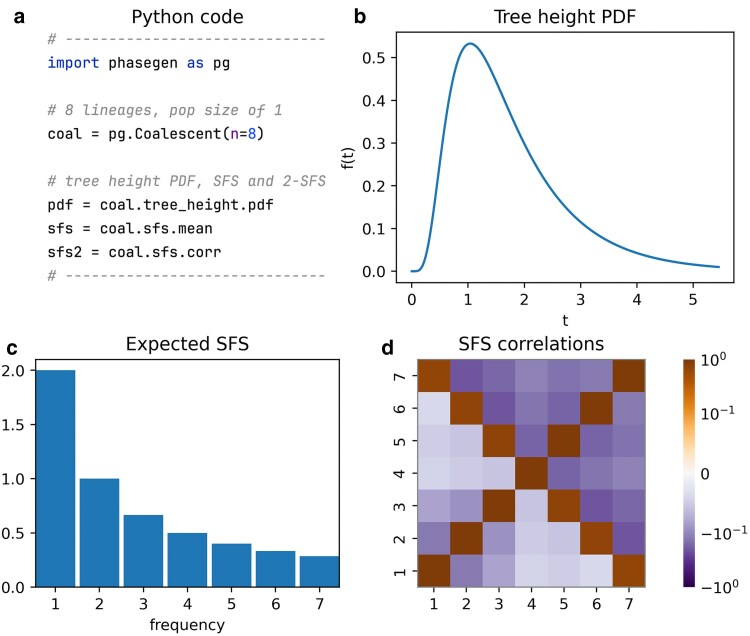 Fig. 1
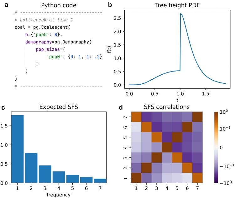 Fig. 2
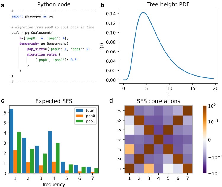 Fig. 3
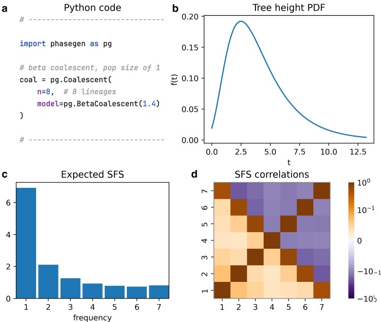 Fig. 4
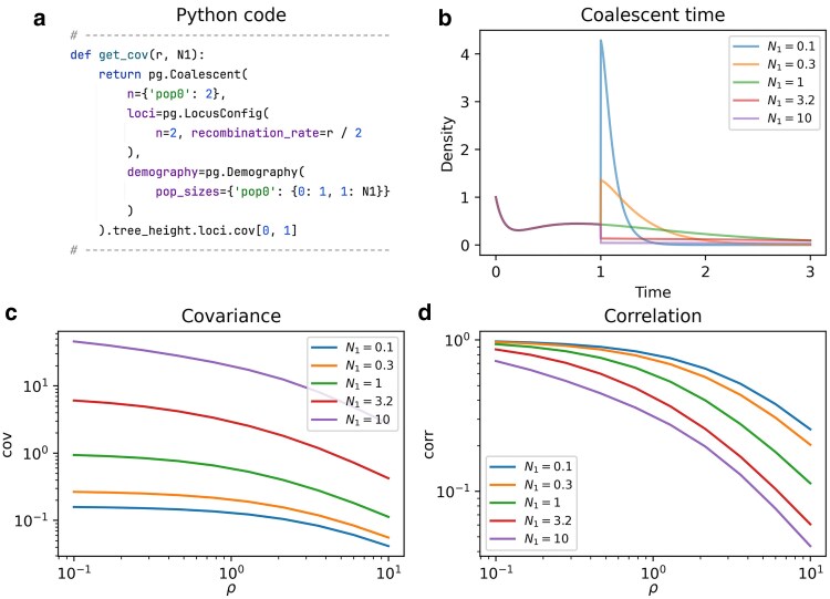 Fig. 5
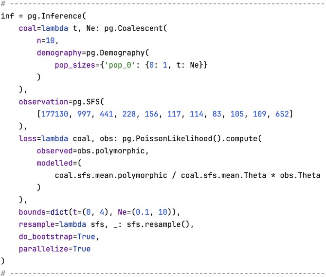 Fig. 6
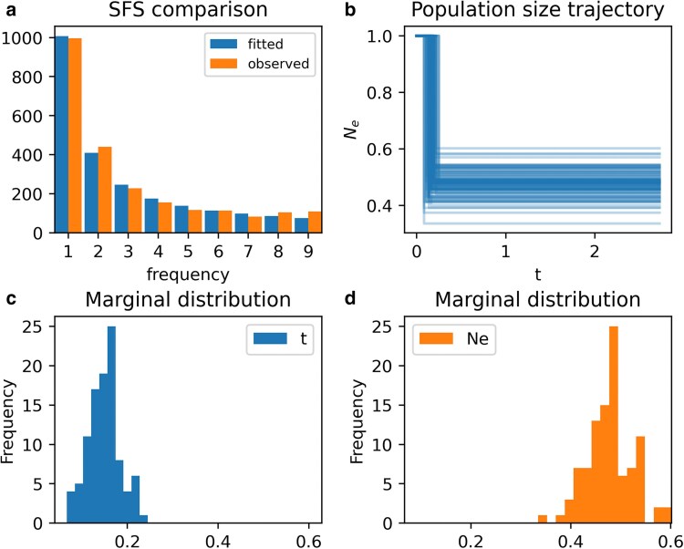 Fig. 7
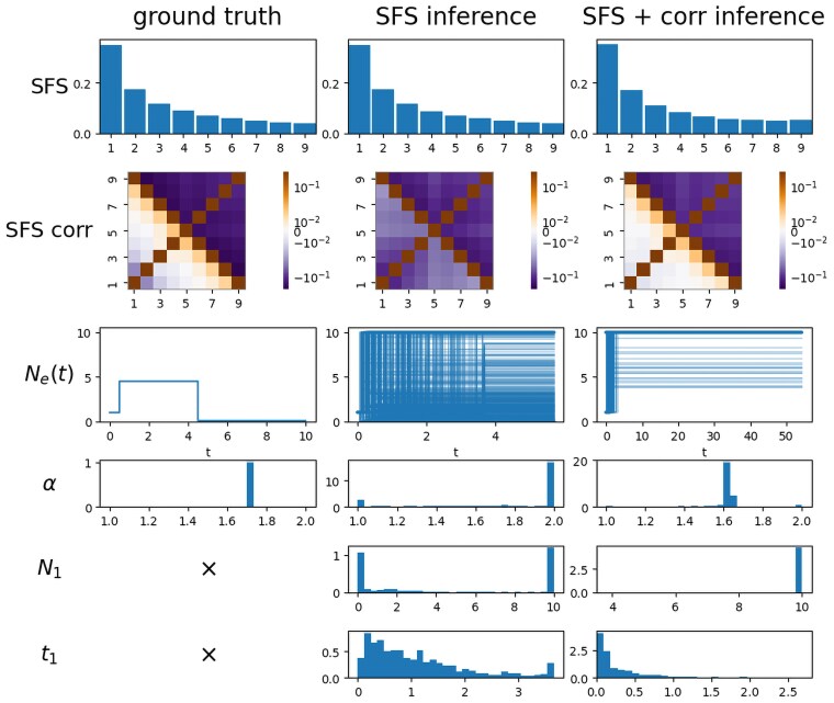 Fig. 8
- —Novo Nordisk Foundation10.13039/501100009708
- —Data Science Collaborative Research Programme
Peer Reviews
No public reviews on file for this paper yet. If you reviewed it on a platform where reviews are public (OpenReview, ICLR, NeurIPS, ICML), you can paste yours below so the community can read it here.
Videos
No videos yet. Explain this paper in a talk, walkthrough, or lecture? Add one.
Taxonomy
TopicsEcology and Vegetation Dynamics Studies · Insurance, Mortality, Demography, Risk Management · Wildlife Ecology and Conservation
Introduction
Population genetics modeling software is essential in evolutionary biology, enabling researchers to explore complex demographic scenarios, evaluate evolutionary hypotheses, and estimate parameters within specified demographic models. A wide range of tools is available, utilizing either backward or forward simulations, with varying levels of support for parameter estimation.
Current coalescent-based simulators, such as msprime, generate stochastic tree sequences, offering significant flexibility while closely reflecting the data generation process (Baumdicker et al. 2021). However, their stochastic nature necessitates numerous replicates to obtain reliable estimates of summary statistics, especially when dealing with complex demographic models or statistics involving higher-order moments (Excoffier et al. 2013). Additionally, this inherent stochasticity complicates the use of gradient-based parameter estimation methods, often leading to the reliance on approximate Bayesian computation (ABC) (Kelleher and Lohse 2020).
Another widely used category of tools is forward simulators, which offer the notable advantage of being able to incorporate selection (Gutenkunst et al. 2009; Jouganous et al. 2017; Haller and Messer 2023). However, forward simulators have their own caveats—notably determining an optimal runtime to reach equilibrium—and demographic models are often easier to specify in a coalescent framework. Tools such as dadi and moments, rely on diffusion-based computations and provide exact solutions for a variety of summary statistics (Gutenkunst et al. 2009; Jouganous et al. 2017). Yet, closed-form solutions to the underlying differential equations are generally unavailable, requiring numerical approximations that can cause instabilities and complicate the computation of higher-order moments (Jouganous et al. 2017). SLiM, by contrast, explicitly tracks each individual in a population, offering high customizability and full access to evolutionary history (Haller and Messer 2023). This level of detail, however, comes at the cost of increased computational complexity, which may be unnecessary for analyses focused solely on summary statistics. Moreover, as with msprime, SLiM simulations are stochastic and require many replicates for robust summary statistics estimation.
Phase-type theory presents a unified framework for modeling mixtures and convolutions of exponential distributions (Bladt and Nielsen 2017). It offers a complementary method to the above approaches by providing exact, numerically stable solutions for a range of coalescent tree statistics (Hobolth et al. 2024). Phase-type theory models the coalescent process as a continuous-time Markov chain, with states representing the possible configurations of lineages in a population. Several software packages have been developed to support its application in population genetics. PhaseTypeR provides a general framework for utilizing phase-type distributions, with a focus on population genetics applications (Rivas-González et al. 2023). In PtDAlgorithms, the emphasis is on accelerating computations by employing a graph-based approach (Røikjer et al. 2022). However, these tools typically require a solid understanding of the underlying theory, with state space construction often left to the user. Additionally, they offer only limited support for time-inhomogeneous coalescent processes, such as those involving changing population sizes or migration rates. Recently, Wences et al. (2025) demonstrated how to derive the distribution and moments of the TMRCA under various time-inhomogeneous coalescent models using phase-type theory. However, available quantities are limited to the TMRCA, and no software implementation is provided.
Here, we introduce PhaseGen, which supports the computation of branch length moments under piecewise-constant demographies. Branch length moments include quantities such as the expected length, variance, and correlation between the lengths of specific branches in a coalescent tree, and are key determinants of the patterns of polymorphism observed in genetic data. PhaseGen is particularly well-suited for optimizing demographic models in a coalescent framework, especially when multiple-merger coalescents (MMCs) are involved. It is also valuable for new methods that rely on exact coalescent-based solutions, making it unnecessary to rederive these quantities. The framework is also well-suited for exploratory analyses, where rapid model specification and easy access to a wide range of summary statistics are beneficial.
The paper begins with an overview of PhaseGen’s implementation, followed by computation and parameter estimation examples that demonstrate its capabilities. We then discuss potential future applications and perspectives on phase-type theory and software in population genetics. In addition, Appendix A presents linear algebraic computation examples (Figs. A1–A3), followed by the theoretical framework for time-inhomogeneous phase-type distributions. Subsequent appendices cover the state space and transition rates for various coalescent models (Appendix B, Figs. B1–B9), additional code examples (Appendix C, Figs. C1–C3), state space sizes (Appendix D, Figs. D1 & D2), computation times under different demographic scenarios (Appendix E, Figs. E1 & E2), a comparison with dadi (Appendix F, Figs. F1 & F2, Table F1), and validation against msprime (Appendix G, Fig. G1, Table G1).
Software implementation
PhaseGen is Python-based, although an R interface with usage examples is also available. It works internally by constructing the state space for the specified coalescent scenario, along with the weights associated with each state needed to compute the summary statistic of interest (Appendix A). PhaseGen enables the computation of branch length (cross-)moments of arbitrary order under a variety of coalescent models (Kingman, Beta, and Dirac coalescent) and demographic scenarios. Alternatively, custom weights (i.e. Rewards) can be assigned to each state in the state space, allowing for the computation of targeted quantities such as the time spent in a particular deme (phasegen.rtfd.io/en/v1.0.2/reference/Python/rewards.html). Additional features include access to the cumulative distribution function (CDF), probability density function (PDF), and quantile function for the coalescent tree height. Branch length moments can also be computed over a specified time interval by adjusting start and end times. By progressively increasing the end time, the accumulation of moments over time can also be analyzed.
The software package is equipped with a Demography interface akin to msprime, designed to handle temporal changes, with helper functions available for discretizing continuous demographic functions. To ensure correctness, PhaseGen has been extensively tested against stochastic estimates from msprime, comparing various summary statistics across a wide range of demographic scenarios, with no discrepancies observed (Appendix G). The source code is hosted on GitHub (github.com/Sendrowski/PhaseGen), with comprehensive documentation available at phasegen.readthedocs.io. Installation is possible via the pip and conda package managers.
In PhaseGen, summary statistics under a given demographic model are obtained by creating a Coalescent object—the main entry point for all computations. This object encapsulates the distributional properties of the underlying coalescent process and includes the specified demography (Demography), coalescent model (CoalescentModel), lineage configuration (LineageConfig), locus configuration (LocusConfig), and the resulting state space (StateSpace). The Demography consists of one or more Epochs, within which population sizes and migration rates are constant. Internally, PhaseGen constructs a state space representing the possible States of the coalescent process (Appendix A). For each epoch, the Transition rates between states are computed based on the specified coalescent model and demography. For tree height and total branch length statistics, the LineageCountingStateSpace is used, which tracks the number of lineages over time. For SFS-based statistics, the larger BlockCountingStateSpace is required, which tracks the number of branches subtending i lineages in the coalescent tree. LineageConfig and LocusConfig specify the initial number of lineages in each deme and locus, respectively. Upon creation, the Coalescent object provides access to a variety of statistics, the most commonly used of which are available as cached properties that are evaluated lazily, i.e. computed only upon access and reused thereafter. This includes branch length moments of the tree height (TreeHeightDistribution), total branch length (total_branch_length), and the site frequency spectrum (UnfoldedSFSDistribution and FoldedSFSDistribution). In addition, TreeHeightDistribution supports computing the CDF, PDF, and quantile functions. For more complex statistics, Rewards can be used to assign weights to states in the state space and passed to the Coalescent.moment function. For further details, please refer to the online reference, accessible through the monospaced terms linked in the text.
We next showcase the capabilities of PhaseGen, beginning with the computation of summary statistics under the Kingman coalescent (Standard coalescent). We then explore more complex scenarios, including piecewise-constant demographies (Multiple epochs), migration (Isolation with migration), multiple-merger coalescents (Multiple-merger coalescents), and recombination (Coalescent with recombination). Finally, we illustrate the use of PhaseGen for parameter estimation (Statistical inference), and demonstrate how higher-dimensional summary statistics can improve inference accuracy (Inference on SFS correlation).
Standard coalescent
In this example, we define a Kingman coalescent model with lineages, and a constant population size of (Wakeley 2009). Note that in most examples we use a population size of 1 for brevity, since coalescent rates scale linearly with N. Figure 1 displays the tree height density, expected SFS, and SFS correlation matrix, along with the code used to define the model and compute these statistics. We create a Coalescent object using the standard coalescent model with a single population of size 1, both of which are default settings. The tree height density (coal.tree_height.pdf), expected SFS (coal.sfs.mean), and SFS correlation matrix (coal.sfs.corr) are then directly accessible. See Inference on SFS Correlation for a more detailed introduction to SFS correlations. Note that while these estimates are based on branch lengths, they can be scaled by the mutation rate to derive the expected number of observed mutations under the infinite-sites model.
Kingman coalescent model with n=8 lineages and constant population size N=1. a) Python code snippet defining the coalescent object for this scenario, and accessing the tree height density, expected SFS, and SFS correlation matrix (cf. plot_manuscript_kingman_example.py, containing the full code to generate the figure). b) Tree height density (PDF). c) Expected SFS. d) (symmetric) SFS correlation matrix representing the branch length correlation of branches subtending i and j lineages in the coalescent tree.
Multiple epochs
Piecewise-constant demographic models can be specified using a Python dictionary that maps time points to population sizes. In this example, we define a 2-epoch model where the population size decreases backward in time from to at . Figure 2 shows the tree height density, expected SFS, and SFS correlation matrix for this model, along with the code used to define the Coalescent object. The population size decrease leads to a higher coalescent rate at time , as reflected in the tree height density. The expected SFS shows a relative excess of singleton variants, due to relatively longer terminal branches resulting from the initially larger population size.
Two-epoch demography featuring a population size reduction backward in time. a) Python code snippet defining the coalescent object for this scenario (cf. plot_manuscript_2_epoch_example.py, containing the full code to generate the figure). The dictionary defines the population sizes, where keys represent time points, and values specify the corresponding population sizes. The identifier pop0 is used for the single population. b) Tree height density (PDF), highlighting a sudden increase in the coalescent rate due to the population size reduction. c) Expected SFS, showing a relative deficit of high-frequency variants. d) SFS correlation matrix.
Isolation with migration
We can also define demes and specify migration between them (Hey 2009). In this example, we model two demes, pop0 and pop1, with population sizes 1 and 2, respectively (Fig. 3). Migration occurs backwards in time at a per-generation rate of from pop0 to pop1. Both demes begin with lineages in the present. Here, we also marginalize the SFS over demes, i.e. we weight the branch lengths by the proportion of lineages spent in each deme over time. In this example, branches are longer for lineages in deme pop1 due to its larger population size and thus lower coalescent rate. Also note that the resulting SFS shows an excess of quadrupletons, which corresponds to relatively longer branches subtending four lineages in the coalescent tree. This pattern arises because lineages are likely to coalesce within their deme of origin prior to migration. We also observe a positive correlation between singletons and tripletons in the SFS correlation matrix (Fig. 3d). Note that the SFS correlation matrix is not to be confused with the joint-SFS, which records the co-occurrence of allele frequency counts across demes.
Two-deme model with uni-directional migration. a) Python code snippet defining the coalescent object for this scenario (cf. plot_manuscript_migration_example.py, containing the full code to generate the figure). The first element of the migration rate tuple specifies the source deme (pop0), and the second specifies the target deme (pop1) backwards in time. b) Tree height density (PDF). c) Total expected SFS and deme-specific contributions. d) SFS correlation matrix.
Multiple-merger coalescents
PhaseGen also supports multiple-merger coalescents (MMCs), where more than two lineages can coalesce simultaneously (see Inference on SFS Correlation for a more detailed introduction to MMCs). Here, we illustrate the BetaCoalescent model, where the probability of coalescence of a fraction of the lineages is determined by a beta distribution parameterized by α, ranging from 1 (star-like coalescent) to 2 (Kingman coalescent) (Schweinsberg 2003). In this example, , leading to frequent coalescence events involving more than two lineages (Fig. 4). The resulting expected SFS shows a relative excess of high-frequency variants, and the SFS correlation matrix reveals positive correlations between branches of different frequency bins—both typical signatures of MMCs.
Beta coalescent model with α=1.4, n=8 lineages, and constant population size N=1. a) Python code snippet defining the coalescent object for this scenario (cf. plot_manuscript_mmc_example.py, containing the full code to generate the figure). b) Tree height density (PDF). Note that unlike for the Kingman coalescent, the TMRCA may be very close to zero. c) Expected SFS which is characterized by a relative deficit of doubletons and an excess of high-frequency variants. d) SFS correlation matrix showing a positive correlation between branches of different frequency bins.
All dynamics presented so far can be combined into a single model (see Appendix C.1 for a more complex example).
Coalescent with recombination
There exist simple closed-form solutions for the covariance of the TMRCAs between two loci depending on the recombination rate ρ. Specifically, for two lineages, the covariance is given by
where both loci are assumed to be initially linked (cf. Formula 7.28 in Wakeley 2009). Here, is the scaled recombination rate, with r denoting the per-generation probability of recombination between the two loci.
To explore this further, we compute the tree height covariance under a time-inhomogeneous demographic model. Figure 5 illustrates the covariance under a 2-epoch model where the population size changes from 1 to at time . For fixed ρ, larger population sizes lead to a higher covariance due to the linear increase in TMRCA with population size. In contrast, the correlation decreases with increasing ρ as higher recombination rates introduce more opportunities for recombination events. This relationship is largely unaffected by the time-inhomogeneous demography. Note that SFS-based summary statistics are currently not supported for multiple loci, since this would require a more complex state space (cf. Discussion).
2-epoch demography with a population size change from 1 to N1 at time t=1. a) Python function to compute the covariance of the TMRCAs depending on ρ and N1 (cf. plot_manuscript_recombination_example.py, containing the full code to generate the figure). Note that ρ is scaled differently in PhaseGen, hence the division by 2. b) Tree height densities for the total TMRCA of both loci for different values of N1 and ρ=10. Note the initial slump in probability mass, which is due to recombination occurring before coalescence. c) Covariance of the TMRCAs for different values of ρ and N1. d) Correlation of the TMRCAs, which ranges from 1 for low ρ to 0 for high ρ. Note that the covariance increases with N1, while the correlation decreases.
Statistical inference
We begin by establishing a connection between the SFS computable from real data and the SFS provided by PhaseGen. The site frequency spectrum (SFS) is a summary statistic that records the frequencies of alleles at sites in a sample of n individuals. That is, each entry k in the SFS counts the number of sites where the derived allele appears in exactly k individuals. Under the infinite-sites model, each site is assumed to experience at most one mutation, so the frequency of a derived allele at a site is directly related to the structure of the underlying coalescent tree—specifically, to the number of terminal branches subtended by the branch where the mutation occurred. The coalescent tree is shaped by selection and demography, but also reflects variation from the stochastic nature of the coalescent process. By averaging over many sites, and assuming sufficient recombination, we reduce this stochastic noise by effectively sampling many independent realizations of the coalescent process. PhaseGen computes the expected SFS under a specified demographic model, with each frequency bin equal to the total branch length where mutations produce alleles at that frequency. Assuming a constant mutation rate and selective neutrality, mutations follow a Poisson process, so that the expected number of mutations at frequency k is given by θ times the total branch length subtending k lineages, where θ is the population-scaled mutation rate. Thus, multiplying the expected SFS from PhaseGen by θ gives the expected SFS observable in real data.
The availability of exact solutions for summary statistics like the SFS lends itself to gradient-based parameter estimation, and thus, PhaseGen provides a compact framework for this purpose. Gradient-based optimization relies on computing the derivative of the loss function with respect to model parameters, enabling navigation toward optimal values via gradient descent. The gradient is often computed numerically because the loss function is usually too complex to differentiate analytically.
Within PhaseGen, parameter inference under a given demographic model can be performed using the Inference class (Fig. 6). This involves defining a function that returns a parameterized Coalescent object (coal). In each optimization iteration, this function is called to obtain the Coalescent object for the current parameter values. In this example, we model a single population size change from size 1 to Ne at time t, where both the time of change t and the resulting population size Ne are variable. This analysis is based on an unfolded SFS obtained from a whole-exome Scandinavian silver birch dataset (Salojarvi et al. 2017; Sendrowski 2022) (observation). Ancestral states were determined using two outgroup species (Alnus incana & A. glutinosa). To evaluate model fit during optimization, we must specify a loss function (loss) which takes two arguments: the observed summary statistic and the parameterized Coalescent object. In this example, the loss function is a composite Poisson likelihood, which assumes that mutations at different frequencies are independent Poisson variables (Poisson random field assumption). To standardize the data, the SFS is normalized by Watterson’s estimator of the population-scaled mutation rate θ. By default, 10 independent optimization runs are carried out with different initial values, and the best result is selected. Optionally, a resampling function can be provided to perform parametric bootstrapping (resample). By default, 100 bootstrap replicates are performed, each initialized with the best fit from the original optimization run. Parameter bounds are set to for t and for Ne (bounds). Note that both t and Ne are expressed in units relative to the effective population size, as both scale linearly with it. The absolute values can be obtained by multiplying the estimates by the effective population size. The inference result is visualized in Fig. 7, and indicates a population size reduction in the past (cf. plot_manuscript_inference_example.py). The inference framework permits an arbitrary parameterization of the coalescent distribution and a customizable choice of loss function, and is thus rather flexible. Additional inference features include support for distributed computing on clusters (cf. the package documentation for more details).
Code snippet for 2-epoch demographic inference. We specify a parameterized Coalescent object (coal), an observed SFS (observation), a Poisson likelihood loss function (loss), parameter bounds (bounds), and a bootstrap resampling function (resample).
a) Comparison between the fitted and observed SFS. b) Population size trajectories derived from the initial parameter estimate and bootstrap replicates, indicating a population size reduction in the past. c & d) Marginal distributions of bootstrap parameter estimates.
The initial optimization took 0.97 s with 103 function evaluations per run, while each bootstrap run averaged 0.3 s and 32 evaluations on a MacBook Pro M2 (cf. Appendix E for a detailed discussion of computation times). Note that computations can be parallelized. For comparison, the same analysis using dadi produced nearly identical results and took 0.71 s with 144 function evaluations per run, and each bootstrap run averaged 0.29 s and 146 evaluations (cf. Fig. F1). In fact, whenever a forward-in-time formulation of PhaseGen’s demography is available, the results should be effectively identical.
Inference on SFS correlation
The following example demonstrates the advantages of including higher-order summary statistics for parameter estimation, with a focus on second-order SFS moments. As a two-dimensional extension of the SFS, the SFS correlation matrix records the correlation between different frequency bins in the SFS, i.e. the branch length correlation of branches subtending i and j lineages in the coalescent tree. In particular, it can reveal signals of multiple-merger coalescents (MMCs), which involve the simultaneous coalescence of more than two lineages (Birkner et al. 2013b). Such events may arise in populations with highly skewed offspring distributions (Eldon and Wakeley 2006). MMCs generate a distinct positive correlation between different SFS frequency bins—a signal that has been shown to be robust to confounding factors such as demographic changes and linkage (Fenton et al. 2025). In practice, SFS correlations can be computed from data by considering the frequencies of pairs of nearby SNPs, assuming independence between sites. Centering and normalizing the raw SFS counts to compute a correlation matrix requires careful consideration of mutational opportunities—i.e. the number of sites where mutations can occur. Alternatively, inference can be performed directly on uncentered moments (see Fenton et al. 2025 for alternative summary statistics and further discussion).
We present a proof-of-concept example using PhaseGen, comparing results from SFS-only inference to those using both the SFS and SFS correlations (Fig. 8). The ground truth in this example assumes a 3-epoch demographic model with a temporary increase followed by a drastic decrease in population size backward in time, and a beta coalescent with , making multiple mergers relatively frequent. More precisely, the population size changes from to at , and subsequently to at . The demographic scenario was specifically chosen to generate an SFS lacking the typical U-shaped profile associated with multiple mergers, making it difficult to infer α from the expected SFS alone. The ground truth SFS and SFS correlations are computed with PhaseGen, assuming sites are unlinked. For inference, a simplified 2-epoch demography is fitted, estimating a population size change from size 1 to at time , alongside α. Note that different models are used for inference and ground truth, introducing noise and reflecting the fact that, in real data, the actual demographic history is more complex than the inference model.
MMC inference results: ground truth (left), SFS-only inference (middle), and inference using both SFS and SFS correlation matrix (right). Rows show the SFS, SFS correlation matrix, population size trajectory, and inferred values for α, N1, and t1, respectively. The demography is challenging to infer from the SFS alone, leading to substantial variability in both estimates of α and the inferred population size history (cf. infer_mmc_kingman_2sfs.py, plot_mmc_inference.py).
A multinomial likelihood is applied to the expected SFS, which is normalized by the total number of polymorphic sites. When incorporating SFS correlations, an additional loss term is added, describing the absolute difference between the observed and modeled correlation coefficient for the fourth and fifth frequency bins. Using only a single correlation coefficient was motivated by performance considerations, and this specific entry was found to be particularly informative. Bootstrapping is performed by applying Poisson sampling to the observed SFS data, generating 1,000 replicates. Figure 8 demonstrates that α is recovered reasonably well when augmenting the loss function with SFS correlation, despite differences between the inference and ground truth demographic models. In contrast, SFS-only inference fails to recover the true value of α, with both α and the inferred population size trajectory showing significant variation across bootstraps. This is because the expected SFS is also sensitive to other demographic effects, making it challenging to disentangle the signal of multiple mergers from the effects of population size changes. For inference incorporating SFS correlations, initial optimization took 29.93 s per run, and each bootstrap run averaged 13.94 s on a MacBook Pro M2.
Discussion
In this work, we introduced PhaseGen, a software package providing an accessible interface for computing exact and numerically stable moments of piecewise-constant coalescent processes under various demographic scenarios. Discrete rate changes are common in population genetics, and can approximate continuous demographies with arbitrary precision.
This framework utilizes Van Loan’s method for computing moments (Appendix A.8), which relies on matrix exponentiation, and for which accurate solutions can be obtained using Padé approximants (Van Loan 1978; Al-Mohy and Higham 2010). Matrix exponentiation generally has a cubic runtime complexity, depending on the sparsity and structure of the matrix. Consequently, it is crucial to keep the state space as small as possible; see Appendix D for state space sizes and Appendix E for corresponding benchmarking results across different configurations.
To address the computational bottlenecks associated with moment and gradient calculations, several strategies may be explored. A graph-based approach, as implemented in PtDAlgorithms, can substantially accelerate moment computations in time-homogeneous settings, although extending this approach to time-inhomogeneous models remains challenging (Røikjer et al. 2022). Alternatively, faster matrix exponentiation algorithms, particularly for sparse matrices or those leveraging the structure of the Van Loan matrix, could offer substantial improvements. While support for GPU-accelerated matrix exponentiation remains limited, it holds potential for significant speedups in the future. Incorporating exact gradient information for parameter estimation is another promising approach that could substantially accelerate optimization algorithms, especially in high-dimensional parameter spaces. Future research could also explore dynamic state space reduction techniques by merging equivalent states or collapsing states with negligible expected sojourn times, depending on the demographic model.
On a related note, the theory of probability generating functions in population genetics (Lohse et al. 2011) is closely tied to phase-type theory (Hobolth et al. 2024). The agemo software package, for instance, utilizes a graph-based approach to compute probabilities for small-sample-size SFS under coalescent-with-migration models (Bisschop 2022). These mutational block configuration probabilities are particularly useful for fitting models to small datasets. PhaseGen also provides phase-type-based support for this, as detailed in Hobolth et al. (2025). However, its current framework is restricted to time-homogeneous demographies, although time-homogeneous dynamics such as migration between demes, and different coalescent models are supported (cf. the package documentation for more details). Extending this functionality to time-inhomogeneous scenarios would significantly broaden its applicability for modeling small-sample data.
Future extensions to PhaseGen could include support for additional structured coalescents, such as models incorporating seed banks, diploidy, and polyploidy. The availability of full distribution functions for rewarded summary statistics, such as the total branch length or the SFS, would also be beneficial. However, to date, this does not appear to be generally possible for time-inhomogeneous models within the phase-type framework. Adding support for SFS-based statistics under the two-locus model would also be valuable, though this would necessitate lineage labeling, leading to a significant increase in state space size, thus making computations infeasible even for moderate lineage counts. Similarly, joint-SFS statistics, which record the co-occurrence of allele frequency counts across different demes, require lineage labeling to track the deme of origin. Finally, a fully labeled state space implementation could enable the calculation of many additional statistics, but computational feasibility would remain a challenge for more than 6–7 lineages, depending on the number of unique labels involved.
PhaseGen can also be used to compute summary statistics under the multi-species coalescent (MSC) model, i.e. by treating each species as a separate deme. Recently, Guerra and Nielsen (2022) derived the covariance of pairwise differences under the MSC model under a piecewise-constant demography, and examined the biases introduced in estimates derived from pairwise differences. While computing the covariance of pairwise differences requires additional lineage labeling, metrics like can be expressed as rational functions of pairwise coalescent times, making them accessible within PhaseGen (Slatkin 1991).
In conclusion, we hope that the software and theory presented here will serve as valuable resources for the population genetics community, facilitating exploratory analyses and the fitting of demographic models to data.
The reference list from the paper itself. Each links out to its DOI / PubMed record.
- 1Al-Mohy AH, Higham NJ. 2010. A new scaling and squaring algorithm for the matrix exponential. SIAM J Matrix Anal Appl. 31:970–989. 10.1137/09074721 X. · doi ↗
- 2Albrecher H, Bladt M. 2018. Inhomogeneous phase-type distributions and heavy tails. J Appl Probab. 56:1044–1064. 10.1017/jpr.2019.60. · doi ↗
- 3Baumdicker F et al 2021. Efficient ancestry and mutation simulation with msprime 1.0. Genetics. 220:iyab 229. 10.1093/genetics/iyab 229. · doi ↗
- 4Birkner M, Blath J, Eldon B. 2013 a. An ancestral recombination graph for diploid populations with skewed offspring distribution. Genetics. 193:255–290. 10.1534/genetics.112.144329.23150600 PMC 3527250 · doi ↗ · pubmed ↗
- 5Birkner M, Blath J, Eldon B. 2013 b. Statistical properties of the site-frequency spectrum associated with Λ-coalescents. Genetics. 195:1037–1053. 10.1534/genetics.113.156612.24026094 PMC 3813835 · doi ↗ · pubmed ↗
- 6Bisschop G . 2022. Graph-based algorithms for Laplace transformed coalescence time distributions. P Lo S Comput Biol. 18:e 1010532. 10.1371/journal.pcbi.1010532.36108047 PMC 9514611 · doi ↗ · pubmed ↗
- 7Bladt M, Nielsen BF. 2017. Matrix-exponential distributions in applied probability. Probability theory and stochastic modelling. Springer.
- 8Eldon B, Wakeley J. 2006. Coalescent processes when the distribution of offspring number among individuals is highly skewed. Genetics. 172:2621–2633. 10.1534/genetics.105.052175.16452141 PMC 1456405 · doi ↗ · pubmed ↗