Do current biomass equations for Alnus glutinosa and Betula pubescens misestimate carbon stocks at peatland sites?
Henriette Gercken, Marius Möller, Ana Lucia Mendez Cartin, Judith Bielefeldt, Emilia Wolfram, Nicole Wellbrock, Julian Gärtner, Cornelius Oertel

TL;DR
This study examines if current biomass equations misestimate carbon stocks in peatland forests in Germany for two tree species.
Contribution
The study evaluates the accuracy of existing biomass equations for peatland sites and compares them with alternative allometric functions.
Findings
Trees in peatland sites show lower heights and biomass at a given diameter compared to mineral soil sites.
The standard biomass equation aligns closely with mean estimates for both species at the stand level.
Peatland-specific equations show high variability and no clear advantage over the standard equation.
Abstract
Accurate estimation of forest carbon stocks is essential for climate change mitigation, particularly in peatland ecosystems known for their high soil organic carbon content. However, biomass equations currently used in Germany, such as the “regular” biomass equation of the National Forest Inventory integrated in the TapeS R package, are primarily calibrated for mineral soil sites and may misestimate biomass in peatland forests. This study evaluates the applicability of existing biomass equations for Alnus glutinosa and Betula pubescens in forested peatlands across Germany by comparing estimates of the biomass equation of the National Forest Inventory with a set of alternative allometric functions, including peatland-specific equations. Using data from 65 forests at peatland and 1266 forests at mineral soil sites, we assessed tree growth patterns, aboveground biomass, and carbon stocks.…
Genes, proteins, chemicals, diseases, species, mutations and cell lines named across the full text — each resolved to its canonical identifier and authoritative record.
Click any figure to enlarge with its caption.
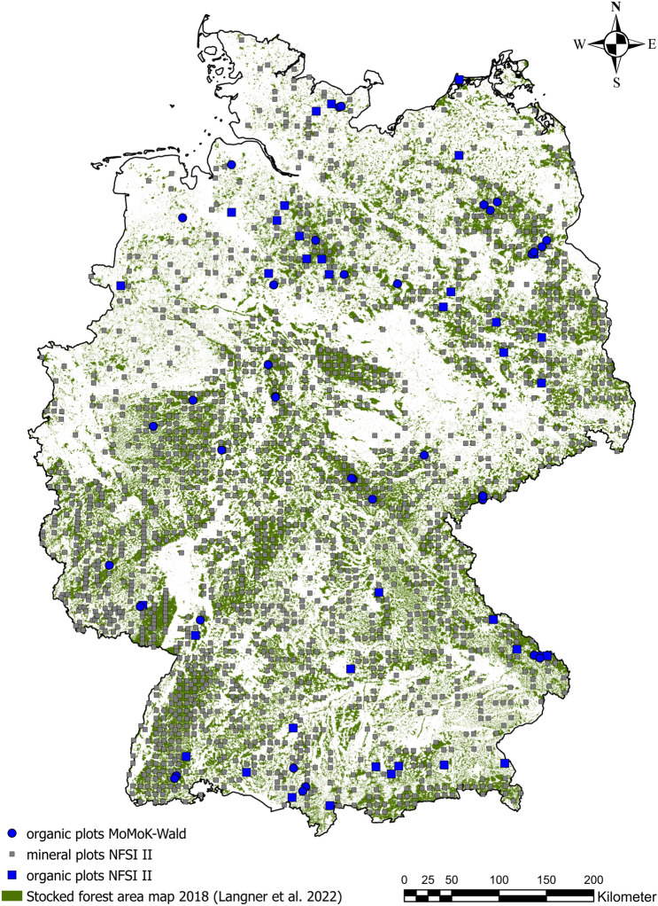 Figure 1
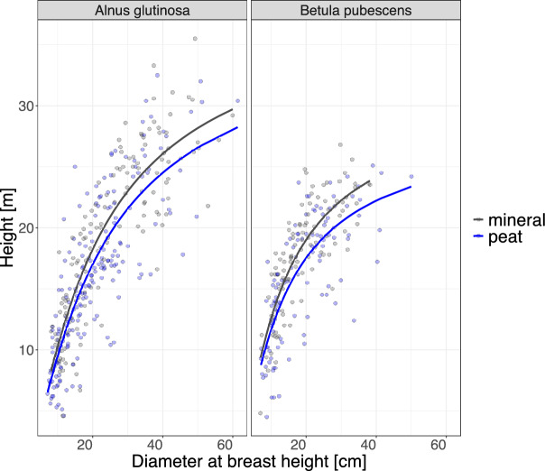 Figure 2
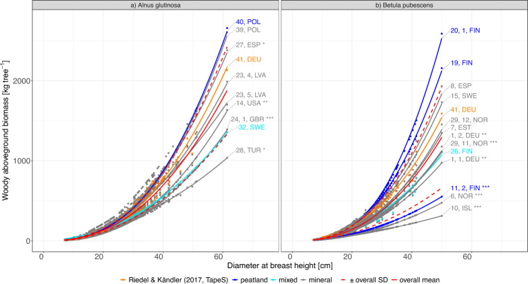 Figure 3
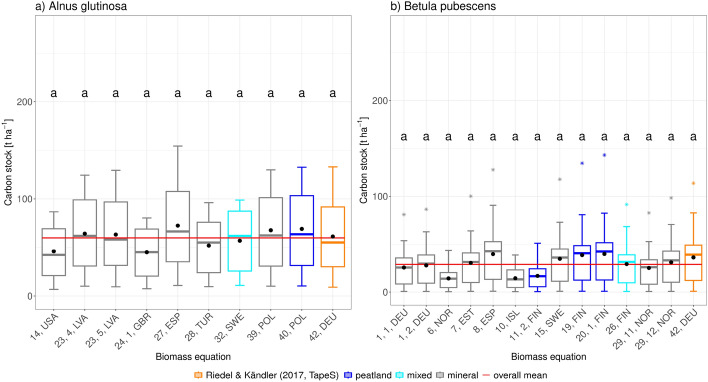 Figure 4
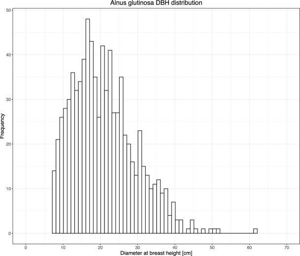 Figure 5
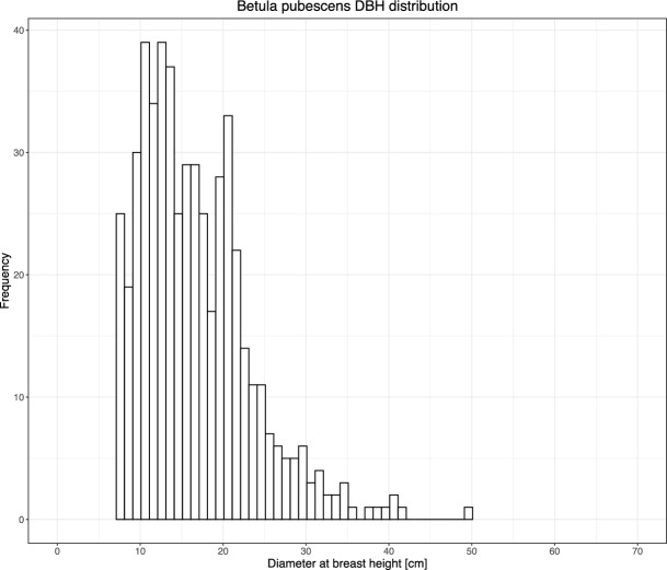 Figure 6
- —Johann Heinrich von Thünen-Institut, Bundesforschungsinstitut für Ländliche Räume, Wald und Fischerei (4249)
Peer Reviews
No public reviews on file for this paper yet. If you reviewed it on a platform where reviews are public (OpenReview, ICLR, NeurIPS, ICML), you can paste yours below so the community can read it here.
Videos
No videos yet. Explain this paper in a talk, walkthrough, or lecture? Add one.
Taxonomy
TopicsPeatlands and Wetlands Ecology · Forest ecology and management · Forest Ecology and Biodiversity Studies
Introduction
Climate change poses an increasing threat to the global ecosystem and human well-being, by directly impacting forest growth and provision of ecosystem services [54, 58, 64]. Therefore, effective mitigation and adaptation measures are urgently needed to prevent its worst impacts [54, 58, 87]. Multiple international conventions have urged signing countries to minimize the causes of climate change by tackling pollution sources and enhancing forest capacity to sequestrate carbon (C) [87, 88]. In the European Union, member states are obliged to make considerable efforts to reduce greenhouse gas (GHG) emissions, as they aim to achieve climate neutrality by 2050 [13, 87, 88]. Forests are essential for GHG reduction because of their crucial role in global carbon dynamics, as they not only absorb billions of tons of CO_2_ annually but also constitute one of the worlds largest terrestrial carbon pools, storing between 70–90% of terrestrial biomass [28, 51]. Therefore, forest policies in the European Union aim for both, the increment of forest cover and carbon sequestration through forest management [18].
In addition, there is a growing societal demand for forests to provide ecosystem services beyond timber production[15, 20, 59], This has led to a revaluation of forests regulation services, such as carbon sequestration [15, 20, 59]. However, the ability of a forest to provide ecosystem services strongly depends on the applied management regime [15, 60, 79]. In this regard, close-to-nature management practices and ecosystem conservation have proven particularly effective in increasing the C sink function of forests while simultaneously improving the provision of other ecosystem services demanded by society [15, 51, 59, 60]. This has led to a general shift from one-purpose, wood production-oriented forestry towards multi-purpose, integrated forest management [20], which can favor undervalued forests, such as peatlands and Betulas spp. and Alnus spp. dominated forests.
Forested peatlands can store twice as much carbon as regular forests by accumulating peat from dead plant material that removed CO_2_ from the atmosphere [10, 30, 46, 82, 89]. Thus, the enormous carbon sequestration potential of peatlands results from their thick peat layer that comprises more than 30% of soil organic matter (SOM), containing approximately 50% of soil organic carbon (SOC) [2, 17, 47]. Although the role of peat SOC in mitigating climate change is becoming increasingly important, the above-ground carbon dynamics of peatland forest communities have been widely disregarded in the past [5, 57, 62, 82]. Therefore, to track and manage how forests affect climate change, accurate ways of quantifying tree biomass are needed.
Allometric functions are a well-established tool in forest yield science to describe growth dynamics and quantify tree stocks. Since they are used primarily to plan timber production, they typically focus on the main commercially relevant species and estimate volume rather than biomass [95]. In light of climate change as a growing threat and stricter international obligations for GHG reporting, functions estimating single-tree biomass have become more relevant [7, 39, 87, 88]. Yet, for forested peatlands most studies and models focus primarily on carbon stored in the peat-body itself [5, 57], where the wet, acidic and extremely nutrient-poor soil conditions lead to very low productivity, rendering these stands nearly irrelevant for timber production and inaccessibly for timber harvest [38, 53, 61, 82]. Additionally, available research on forested peatlands comes primarily from countries in the boreal region, where a large proportion of peatlands used for forestry are drained for this purpose [82].
Therefore, biomass functions for typical forest communities of intact peatlands are hardly available and, if so, they fail to represent peatland growing conditions.
In temperate regions, currently ongoing peatland re-naturation efforts are likely to cause the re-establishment of site-adapted peat forest communities [7, 16] which are typically dominated by water-tolerant species such as Alnus glutinosa and Betula pubescens [16]. Most biomass equations for these species are found for Scandinavian countries such as Finland [32–34, 65], Sweden [43, 45] and Norway [8, 81]. In temperate regions, peatland-specific equations were found for Poland [94], the USA [42] and England [29]. Yet, there is an absence of available functions that explicitly represent the growth of peatland forest communities in Germany. Therefore, biomass in peatland forests is estimated using the “regular” biomass equation of the German National Forest Inventory (NFI) which is also used to account for the carbon balance of the country’s forest sector (hereafter referred to as equation 41, DEU) [24, 68, 90]. This overall aboveground biomass equation, in the case of Betula pubescens (B. pubescens) and Alnus glutinosa (A. glutinosa), uses coefficients for a whole group of species, instead of calculating species-specific coefficients for each of them [67, 90, 91]. These coefficients are parametrised based on pseudo-observations originating from yield tables by Grundner and Schwappach [26], which are not only outdated but were also developed for mineral sites [26, 63, 67]. Therefore, applying this biomass function to peatland forests can carry uncertainty on the accuracy of its predictions. However, its comparability with past and future National Forest Inventories (NFI), National Forest Soil Inventories (NFSI), and National Greenhouse Gas Reporting argues in favour of its use. Still, other biomass functions have been found to estimate biomass of B. pubescens in Germany, but they focus on mineral soils of a specific region [3]. Similarly to A. glutinosa, whose main base of species-specific biomass estimations are region specific yield tables developed by Lockow et al.[56] for Northeast Germany. Therefore, the resulting lack of extrapolation capacity may not allow for these equations or tables to be used on a broader scale.
The lack of a species-specific equation parametrised on a national level limits the current peatland forest carbon estimation in Germany, as, to our knowledge, none of the available functions are developed or validated with real peatland forest biomass data, nor tested with other peatland biomass specific equations to determine their predictive capacity. The increasing importance of peatland forests C stocks and the simultaneous uncertainty associated with current C assessments in these ecosystems create a need to increase the accuracy of biomass estimations [7]. Therefore, our study aims to assess the predictive capacity of the 41, DEU function currently used to calculate C stocks in Germany, by comparing its predictions with those of peatland- and species-specific equations parametrised for several extratropical areas. We aim to answer the research question of whether the 41, DEU equation is capable of predicting biomass stocks similar to peatland-specific equations. We hypothesised that (1) the growth dynamics of forest communities differ significantly between peatland and mineral sites and (2) hence the existing 41, DEU cannot be applied to peatland forests of A. glutinosa and B. pubescens without adjustments. Further, we assume that (3) the 41, DEU equation’s predictors are dissimilar to the peatland-specific equations, causing the overestimation of carbon stocks compared to equations created for peatlands in temperate regions and the overall mean of all peatland- and species-specific equations.
Methods
Study area
The study includes sites throughout the entire territory of Germany, a country situated in Central Europe between latitudes 47° and 55° N and longitudes 5° and 15° E. Germany features a temperate seasonal climate, with generally humid conditions, mild to warm summers, and cool winters. Annual precipitation varies regionally, but typically ranges between 500 and 1000 mm, supporting diverse forest types, ranging from the Picea abies or Abies alba dominated mountain forests in subalpine regions over deciduous forests dominated by Fagus sylvatica in central Germany to Alnus glutinosa and Alnus incana, Betula pubescens or Pinus sylvestris peatland forests concentrated in the north German plain [77, 86]. Forests cover around 30% of the country’s surface area and consists mainly of of temperate broad-leafed and mixed forests and managed woodlands [69, 92]. However, due to commercial purposes, the most common species are currently Pinus sylvestris and Picea abies, followed by Fagus sylvatica and Quercus spp. [69]. The main coniferous species are also found in peatlands, where they represent the predominant tree species together with Betula pubescens and Alnus glutinosa [16]. Peatlands in Germany cover approximately 1.8 million hectares, which represents approximately 5% of the country’s surface area [7], where about 15% are forested [7].
This study focuses specifically on plots throughout Germany that contain A. glutinosa and B. pubescens, which occur at peatland as well as mineral soil sites. A. glutinosa account for 2.6% of Germany’s forest cover [84] and thrive at sites with high water saturation up to periodic flooding and water stagnation, because of their high tolerance to waterlogging [21, 38, 78]. Due of their moderate requirements in terms of base and nutrient supply, they are displaced by B. pubescens in heavily acidified, nutrient-poor locations [21, 78]. Trees of the botanical genus Betula cover 4.7% of the countries forest area [84], whereby the distribution of B. pubescens concentrates on acidic peatland sites [6, 78].
Selection of biomass equations
In order to compare the predictive capacity of 41, DEU to the results of other species- and peatland specific biomass equations we carried out a literature review to collect allometric functions for A. glutinosa and B. pubsecens. Since water table fluctuations are the main driver of tree growth dynamics at peatland forests [4, 53, 66, 71, 72] and drainage promotes tree growth [53, 66], we assume that tree growth will become increasingly detached from the hydrological regime and approximate the growth dynamics at mineral sites. Therefore, we have included equations that originate from peatlands and mineral sites to take into account the fact that most peatlands in Germany have been drained [7].
The following keywords were used for the search: “biomass function alnus glutinosa”, “biomass equation alnus glutinosa”, “biomass alnus glutinosa”, “biomass allocation alnus glutinosa”, “biomass function betula pubescens”, “biomass equation betula pubescens”, “biomass betula pubescens” “biomass allocation betula pubescens”. Publications were included in the analysis only if (1) the relevant keywords appeared in the title, abstract, or listed keywords, (2) the equations originate from extratropical regions, and (3) they presented equations and parameters to estimate the woody above-ground biomass of individual trees (WAG) based on diameter at breast height (DBH, cm) and height (H, m). The tree compartment “foliage” had to be excluded from the aboveground biomass equations sourced from the literature review to ensure better comparability with equation 41, DEU. Therefore, we excluded those functions that included foliage in their calculation, as 41, DEU only accounts for the aboveground woody tree compartments. Additionally, we only considered equations that were species specific for A. glutinosa and B. pubsecens.
This selection returned a final set of seven publications for A. glutinosa [29, 43, 49, 55, 74, 76, 94] and 11 publications concerning B. pubescens [3, 8, 11, 27, 31–34, 44, 65, 81], that provided a biomass equation to calculate the total WAG or equations for the trees woody compartments that were then summarised to extrapolate the WAG (Table 1).Table 1. Overview of biomass equations sourced from literature review with their reference (“reference”) for Betula pubescens and Alnus glutinosa (“species”).IDSpeciesCountryVariablesCompartmentPeatReference1, 1, DEUBetulaGermanyDBH**WAGminAlbert et al. [3]1, 2, DEUBetulaGermanyDBH,H**WAGminAlbert et al. [3]6, NORBetulaNorwayDBH**SW^1^minBollandsås et al. [8]7, ESTBetulaEstoniaDBH**SW+SWBminBuht et al. [11]8, ESPBetulaSpainDBH,H SWB + SWB + FWBminGómez-García et al. [27]10, ISLBetulaIslandDBH** SWB + FWBminHunziker [31]11, 2, FINBetulaFinlandDBH**WAGpeatHytönen and Saarsalmi [34]19, FINBetulaFinlandDBH** SW + FWBpeatHytönen and Aro [32]20, FINBetulaFinlandDBH**WAGpeatHytönen and Kaunisto [33]15, SWEBetulaSwedenDBH**SW + SWB + FWB minJohansson [43]26, FINBetulaFinlandDBH,H SW + SWB + FWB + STWmixRepola [65]29, 11, NORBetulaNorwayDBH** SW + SWB + FWBminSmith et al. [81]29, 12, NORBetulaNorwayDBH,H* SW + SWB + FWBminSmith et al. [81]14, USAAlnusUSADBH* SW + SWBminJenkins et al. [42]23, 4, LVAAlnusLatviaDBH,H**WAGminLiepiņš et al. [55]23, 5, LVAAlnusLatviaDBH,H**WAGminLiepiņš et al. [55]24, 1, GBRAlnusUnited KingdomDBH**WAGminHughes [29]27, ESPAlnusSpainDBH, H SW + FWBminRuiz-Peinado Gertrudix et al. [75]28, TURAlnusTurkeyDBH,H SW + SWB + FWBminSaracoglu [76]32, SWEAlnusSwedenDBH** SW + FWBmixJohansson [44]39, POLAlnusPolandDBH SW + SWB + FWBminWojciech [94]40, POLAlnusPolandDBH** SW + SWB + FWBpeatWojciech [94] \documentclass[12pt]{minimal} \usepackage{amsmath} \usepackage{wasysym} \usepackage{amsfonts} \usepackage{amssymb} \usepackage{amsbsy} \usepackage{mathrsfs} \usepackage{upgreek} \setlength{\oddsidemargin}{-69pt} \begin{document}$$^1FWB$$\end{document} available but not included since it was provided as “crown” consisting of woody compartments and leaf massColumn “ID" refers to the subsequent number of the publication, number of equation (if there were multiple equations per publication) and the country (“country") the equation originates from. Variables required to apply the equation are presented in “variables". “Peat" shows the site type the equation was parametrised for, “min" being mineral sites, “peat" are peatland sites, and “mix" reffers to euqations that were developed with data from both site types. Information about the tree compartments used to calculate the are reported in “compartment" where “WAG" refers to the total woody aboveground biomass, “SW" is stemwood, “SWB" is stemwood bark, “STW" is stumpwood, “STB" is stumpwood bark and “FWB" is finewood. All equations as well as more detailed information for each function provided in .
Data acquisition and processing
Data was obtained from the second NFSI and the Peatland Monitoring Program for Climate Protection - Forest project ( \documentclass[12pt]{minimal} \usepackage{amsmath} \usepackage{wasysym} \usepackage{amsfonts} \usepackage{amssymb} \usepackage{amsbsy} \usepackage{mathrsfs} \usepackage{upgreek} \setlength{\oddsidemargin}{-69pt} \begin{document}$$MoMoK-Wald$$\end{document} ). The NFSI II soil data was sampled between 2006 and 2008 [93], while the corresponding stand data was collected between 2011 and 2012 [36]. The forest inventory at \documentclass[12pt]{minimal} \usepackage{amsmath} \usepackage{wasysym} \usepackage{amsfonts} \usepackage{amssymb} \usepackage{amsbsy} \usepackage{mathrsfs} \usepackage{upgreek} \setlength{\oddsidemargin}{-69pt} \begin{document}$$MoMoK-Wald$$\end{document} plots used in this study was carried out between 2021 and 2024 [23].
We extracted the plots located in peatlands from the totality of 1284 NFSI II and 47 \documentclass[12pt]{minimal} \usepackage{amsmath} \usepackage{wasysym} \usepackage{amsfonts} \usepackage{amssymb} \usepackage{amsbsy} \usepackage{mathrsfs} \usepackage{upgreek} \setlength{\oddsidemargin}{-69pt} \begin{document}$$MoMoK-Wald$$\end{document} plots. We selected only those plots that were defined as organic soils by the German soil classification system (KA5) [1] and that also aligned with the IPCC definition for peatland [17, 40]. The IPCC defines peat soils as soils that have an organic horizon of \documentclass[12pt]{minimal} \usepackage{amsmath} \usepackage{wasysym} \usepackage{amsfonts} \usepackage{amssymb} \usepackage{amsbsy} \usepackage{mathrsfs} \usepackage{upgreek} \setlength{\oddsidemargin}{-69pt} \begin{document}$$>=$$\end{document} 10 cm thickness, which contains at least 20 or 35% SOM (12 or 20% SOC) depending on the prevailing water regime and soil texture [17, 40]. While the German classification identifies organic sites by an organic layer \documentclass[12pt]{minimal} \usepackage{amsmath} \usepackage{wasysym} \usepackage{amsfonts} \usepackage{amssymb} \usepackage{amsbsy} \usepackage{mathrsfs} \usepackage{upgreek} \setlength{\oddsidemargin}{-69pt} \begin{document}$$>=$$\end{document} 30 cm, which begins within the first 70 cm below the soil surface and has an SOM content of 30 % ( \documentclass[12pt]{minimal} \usepackage{amsmath} \usepackage{wasysym} \usepackage{amsfonts} \usepackage{amssymb} \usepackage{amsbsy} \usepackage{mathrsfs} \usepackage{upgreek} \setlength{\oddsidemargin}{-69pt} \begin{document}$$SOC>=15~\%$$\end{document} )[2]. Therefore, the IPCC definition includes peatland sites according to the German definition plus a variety of other organic soils that are not included in the peatland German definition [7] (Table 2).Table 2. Comparison of the peatland definition according to the IPCC (“IPCC definition”) and the organic soil definition according to the German soil classification system (“German KA5 definition”).IPCC definition of peat soilsGerman KA5 definition of organic soilsKA5subtypedescription of subtypeIPCC & KA5 match1.Organic horizon \documentclass[12pt]{minimal} \usepackage{amsmath} \usepackage{wasysym} \usepackage{amsfonts} \usepackage{amssymb} \usepackage{amsbsy} \usepackage{mathrsfs} \usepackage{upgreek} \setlength{\oddsidemargin}{-69pt} \begin{document}$$>=10 cm$$\end{document} , if \documentclass[12pt]{minimal} \usepackage{amsmath} \usepackage{wasysym} \usepackage{amsfonts} \usepackage{amssymb} \usepackage{amsbsy} \usepackage{mathrsfs} \usepackage{upgreek} \setlength{\oddsidemargin}{-69pt} \begin{document}$$<20 cm$$\end{document} with \documentclass[12pt]{minimal} \usepackage{amsmath} \usepackage{wasysym} \usepackage{amsfonts} \usepackage{amssymb} \usepackage{amsbsy} \usepackage{mathrsfs} \usepackage{upgreek} \setlength{\oddsidemargin}{-69pt} \begin{document}$$SOC>=12 \%$$\end{document} when mixed to depth of 20 cm2.Never water saturated for more than a few days, \documentclass[12pt]{minimal} \usepackage{amsmath} \usepackage{wasysym} \usepackage{amsfonts} \usepackage{amssymb} \usepackage{amsbsy} \usepackage{mathrsfs} \usepackage{upgreek} \setlength{\oddsidemargin}{-69pt} \begin{document}$$SOC>20 \%$$\end{document} ( \documentclass[12pt]{minimal} \usepackage{amsmath} \usepackage{wasysym} \usepackage{amsfonts} \usepackage{amssymb} \usepackage{amsbsy} \usepackage{mathrsfs} \usepackage{upgreek} \setlength{\oddsidemargin}{-69pt} \begin{document}$$SOM>35 \%$$\end{document} )3.Episodically water saturated anda. Clay proportion \documentclass[12pt]{minimal} \usepackage{amsmath} \usepackage{wasysym} \usepackage{amsfonts} \usepackage{amssymb} \usepackage{amsbsy} \usepackage{mathrsfs} \usepackage{upgreek} \setlength{\oddsidemargin}{-69pt} \begin{document}$$=0 \%$$\end{document} : \documentclass[12pt]{minimal} \usepackage{amsmath} \usepackage{wasysym} \usepackage{amsfonts} \usepackage{amssymb} \usepackage{amsbsy} \usepackage{mathrsfs} \usepackage{upgreek} \setlength{\oddsidemargin}{-69pt} \begin{document}$$SOC>=12 \%$$\end{document} ( \documentclass[12pt]{minimal} \usepackage{amsmath} \usepackage{wasysym} \usepackage{amsfonts} \usepackage{amssymb} \usepackage{amsbsy} \usepackage{mathrsfs} \usepackage{upgreek} \setlength{\oddsidemargin}{-69pt} \begin{document}$$SOM>=20 \%$$\end{document} )b. clay \documentclass[12pt]{minimal} \usepackage{amsmath} \usepackage{wasysym} \usepackage{amsfonts} \usepackage{amssymb} \usepackage{amsbsy} \usepackage{mathrsfs} \usepackage{upgreek} \setlength{\oddsidemargin}{-69pt} \begin{document}$$>=60 \%$$\end{document} : \documentclass[12pt]{minimal} \usepackage{amsmath} \usepackage{wasysym} \usepackage{amsfonts} \usepackage{amssymb} \usepackage{amsbsy} \usepackage{mathrsfs} \usepackage{upgreek} \setlength{\oddsidemargin}{-69pt} \begin{document}$$SOC>=18 \%$$\end{document} ( \documentclass[12pt]{minimal} \usepackage{amsmath} \usepackage{wasysym} \usepackage{amsfonts} \usepackage{amssymb} \usepackage{amsbsy} \usepackage{mathrsfs} \usepackage{upgreek} \setlength{\oddsidemargin}{-69pt} \begin{document}$$SOM>=30 \%$$\end{document} )c. Intermediate clay amount: intermediate, proportional amount SOCorganic horizont \documentclass[12pt]{minimal} \usepackage{amsmath} \usepackage{wasysym} \usepackage{amsfonts} \usepackage{amssymb} \usepackage{amsbsy} \usepackage{mathrsfs} \usepackage{upgreek} \setlength{\oddsidemargin}{-69pt} \begin{document}$$>=30 cm$$\end{document} consiting of peat (H-horizon) containing \documentclass[12pt]{minimal} \usepackage{amsmath} \usepackage{wasysym} \usepackage{amsfonts} \usepackage{amssymb} \usepackage{amsbsy} \usepackage{mathrsfs} \usepackage{upgreek} \setlength{\oddsidemargin}{-69pt} \begin{document}$$SOM>=30 \%$$\end{document} Anmoorgley1. Organic horizont \documentclass[12pt]{minimal} \usepackage{amsmath} \usepackage{wasysym} \usepackage{amsfonts} \usepackage{amssymb} \usepackage{amsbsy} \usepackage{mathrsfs} \usepackage{upgreek} \setlength{\oddsidemargin}{-69pt} \begin{document}$$<40 cm$$\end{document} with \documentclass[12pt]{minimal} \usepackage{amsmath} \usepackage{wasysym} \usepackage{amsfonts} \usepackage{amssymb} \usepackage{amsbsy} \usepackage{mathrsfs} \usepackage{upgreek} \setlength{\oddsidemargin}{-69pt} \begin{document}$$SOM>=15 -<30 \%$$\end{document} 2. Subject to saturation by ground- or backwater close to terrain surfacenoMoorgley1. Peat horizont \documentclass[12pt]{minimal} \usepackage{amsmath} \usepackage{wasysym} \usepackage{amsfonts} \usepackage{amssymb} \usepackage{amsbsy} \usepackage{mathrsfs} \usepackage{upgreek} \setlength{\oddsidemargin}{-69pt} \begin{document}$$>=10-<30 cm$$\end{document} with \documentclass[12pt]{minimal} \usepackage{amsmath} \usepackage{wasysym} \usepackage{amsfonts} \usepackage{amssymb} \usepackage{amsbsy} \usepackage{mathrsfs} \usepackage{upgreek} \setlength{\oddsidemargin}{-69pt} \begin{document}$$SOM>=30 \%$$\end{document} ( \documentclass[12pt]{minimal} \usepackage{amsmath} \usepackage{wasysym} \usepackage{amsfonts} \usepackage{amssymb} \usepackage{amsbsy} \usepackage{mathrsfs} \usepackage{upgreek} \setlength{\oddsidemargin}{-69pt} \begin{document}$$SOC>=15 \%$$\end{document} )2. Long-term saturated by groundwater close to the terrains surfaceyesHochmoor1. Natural peatland2. Develop under influence of rainwater3. Peat horizon \documentclass[12pt]{minimal} \usepackage{amsmath} \usepackage{wasysym} \usepackage{amsfonts} \usepackage{amssymb} \usepackage{amsbsy} \usepackage{mathrsfs} \usepackage{upgreek} \setlength{\oddsidemargin}{-69pt} \begin{document}$$<30 cm$$\end{document} with \documentclass[12pt]{minimal} \usepackage{amsmath} \usepackage{wasysym} \usepackage{amsfonts} \usepackage{amssymb} \usepackage{amsbsy} \usepackage{mathrsfs} \usepackage{upgreek} \setlength{\oddsidemargin}{-69pt} \begin{document}$$SOM>=30 \%$$\end{document} ( \documentclass[12pt]{minimal} \usepackage{amsmath} \usepackage{wasysym} \usepackage{amsfonts} \usepackage{amssymb} \usepackage{amsbsy} \usepackage{mathrsfs} \usepackage{upgreek} \setlength{\oddsidemargin}{-69pt} \begin{document}$$SOC>=15 \%$$\end{document} )yesNiedermoor1. Natural peatland2. Develop under influence of ground- and/or floodwater accumulated at/above terrain surface3. Peat horizon \documentclass[12pt]{minimal} \usepackage{amsmath} \usepackage{wasysym} \usepackage{amsfonts} \usepackage{amssymb} \usepackage{amsbsy} \usepackage{mathrsfs} \usepackage{upgreek} \setlength{\oddsidemargin}{-69pt} \begin{document}$$<30 cm$$\end{document} with \documentclass[12pt]{minimal} \usepackage{amsmath} \usepackage{wasysym} \usepackage{amsfonts} \usepackage{amssymb} \usepackage{amsbsy} \usepackage{mathrsfs} \usepackage{upgreek} \setlength{\oddsidemargin}{-69pt} \begin{document}$$SOM>=30 \%$$\end{document} ( \documentclass[12pt]{minimal} \usepackage{amsmath} \usepackage{wasysym} \usepackage{amsfonts} \usepackage{amssymb} \usepackage{amsbsy} \usepackage{mathrsfs} \usepackage{upgreek} \setlength{\oddsidemargin}{-69pt} \begin{document}$$SOC>=15 \%$$\end{document} )yesErdhochmoor, Erdniedermoor, Mulmniedermoor1. Cultivated peatland2. Peat horizon \documentclass[12pt]{minimal} \usepackage{amsmath} \usepackage{wasysym} \usepackage{amsfonts} \usepackage{amssymb} \usepackage{amsbsy} \usepackage{mathrsfs} \usepackage{upgreek} \setlength{\oddsidemargin}{-69pt} \begin{document}$$SOC>=15 \%$$\end{document} ( \documentclass[12pt]{minimal} \usepackage{amsmath} \usepackage{wasysym} \usepackage{amsfonts} \usepackage{amssymb} \usepackage{amsbsy} \usepackage{mathrsfs} \usepackage{upgreek} \setlength{\oddsidemargin}{-69pt} \begin{document}$$SOM>=30 \%$$\end{document} ), possibly disturbed by mineral layers but total thickness \documentclass[12pt]{minimal} \usepackage{amsmath} \usepackage{wasysym} \usepackage{amsfonts} \usepackage{amssymb} \usepackage{amsbsy} \usepackage{mathrsfs} \usepackage{upgreek} \setlength{\oddsidemargin}{-69pt} \begin{document}$$<30 cm$$\end{document} yes“KA5 subtype” contains the subtypes of organic soils in the KA5, “description of subtype” their characteristics, and “IPCC & KA5 match” gives information about the subtypes compliance with both IPCC and KA5 regulations
This selection resulted in a total of 65 forested peatland sites, consisting of 47 \documentclass[12pt]{minimal} \usepackage{amsmath} \usepackage{wasysym} \usepackage{amsfonts} \usepackage{amssymb} \usepackage{amsbsy} \usepackage{mathrsfs} \usepackage{upgreek} \setlength{\oddsidemargin}{-69pt} \begin{document}$$MoMoK-Wald$$\end{document} plots and 18 NFSIII plots. The remaining 1266 forested NFSI II plots are classified as mineral sites (Fig. 1).Fig. 1. Overview of the sampling plots from NFSI II and \documentclass[12pt]{minimal} \usepackage{amsmath} \usepackage{wasysym} \usepackage{amsfonts} \usepackage{amssymb} \usepackage{amsbsy} \usepackage{mathrsfs} \usepackage{upgreek} \setlength{\oddsidemargin}{-69pt} \begin{document}$$MoMoK-Wald$$\end{document} : Circles represent \documentclass[12pt]{minimal} \usepackage{amsmath} \usepackage{wasysym} \usepackage{amsfonts} \usepackage{amssymb} \usepackage{amsbsy} \usepackage{mathrsfs} \usepackage{upgreek} \setlength{\oddsidemargin}{-69pt} \begin{document}$$MoMoK-Wald$$\end{document} plots, while squares indicate NFSI II plots. Blue colour highlights peatland plots, grey colour refers to mineral soil plots. The green raster depicts a stocked forest area map of 2018 [52].
All plots provided information on DBH (cm), tree age, geographical position, social class, canopy layer for all trees and H (m) for the five most representative individuals of each species, canopy layer and DBH class.
For trees whose diameter could not be measured at a height of 1.3 m, we used equation (eq.) 1 developed by Dahm [14] and adjusted by NFSI [14, 68] to convert the measured diameter into DBH. The results were divided by 10 to transform them to DBH in cm:
\documentclass[12pt]{minimal} \usepackage{amsmath} \usepackage{wasysym} \usepackage{amsfonts} \usepackage{amssymb} \usepackage{amsbsy} \usepackage{mathrsfs} \usepackage{upgreek} \setlength{\oddsidemargin}{-69pt} \begin{document}$$\begin{aligned} DBH = D_{\textrm{m}} + \frac{2 \times (H_{\mathrm{D_{\textrm{m}}}}-130)}{\tan _{\textrm{SP, C}}} \end{aligned}$$\end{document}where, DBH is the estimated diameter at breast height (mm), \documentclass[12pt]{minimal} \usepackage{amsmath} \usepackage{wasysym} \usepackage{amsfonts} \usepackage{amssymb} \usepackage{amsbsy} \usepackage{mathrsfs} \usepackage{upgreek} \setlength{\oddsidemargin}{-69pt} \begin{document}$$D_{\textrm{m}}$$\end{document} is the measured diameter (mm), \documentclass[12pt]{minimal} \usepackage{amsmath} \usepackage{wasysym} \usepackage{amsfonts} \usepackage{amssymb} \usepackage{amsbsy} \usepackage{mathrsfs} \usepackage{upgreek} \setlength{\oddsidemargin}{-69pt} \begin{document}$$H_{\mathrm{D_{\textrm{m}}}}$$\end{document} is the tree height in m at which \documentclass[12pt]{minimal} \usepackage{amsmath} \usepackage{wasysym} \usepackage{amsfonts} \usepackage{amssymb} \usepackage{amsbsy} \usepackage{mathrsfs} \usepackage{upgreek} \setlength{\oddsidemargin}{-69pt} \begin{document}$$D_{\textrm{m}}$$\end{document} was taken and \documentclass[12pt]{minimal} \usepackage{amsmath} \usepackage{wasysym} \usepackage{amsfonts} \usepackage{amssymb} \usepackage{amsbsy} \usepackage{mathrsfs} \usepackage{upgreek} \setlength{\oddsidemargin}{-69pt} \begin{document}$$\tan _{\textrm{SP, C}}$$\end{document} is the tangent specific to species and region.
To obtain the height for all trees in the plots - as the inventories only provide it for few representative trees - we fitted a non-lineal regression model for each species using the R-package “forestmangr” [9]. The model included the H and DBH delivered by the inventories:
\documentclass[12pt]{minimal} \usepackage{amsmath} \usepackage{wasysym} \usepackage{amsfonts} \usepackage{amssymb} \usepackage{amsbsy} \usepackage{mathrsfs} \usepackage{upgreek} \setlength{\oddsidemargin}{-69pt} \begin{document}$$\begin{aligned} H = \beta _\textrm{0} \times (1 - exp( - \beta _\textrm{1} \times DBH_\textrm{cm}))^{\beta _\textrm{2}} \end{aligned}$$\end{document}where H is the estimated height (m), \documentclass[12pt]{minimal} \usepackage{amsmath} \usepackage{wasysym} \usepackage{amsfonts} \usepackage{amssymb} \usepackage{amsbsy} \usepackage{mathrsfs} \usepackage{upgreek} \setlength{\oddsidemargin}{-69pt} \begin{document}$$DBH_\textrm{cm}$$\end{document} corresponds to the diameter at breast height (1.3m) in cm for all trees - with and without height information - and \documentclass[12pt]{minimal} \usepackage{amsmath} \usepackage{wasysym} \usepackage{amsfonts} \usepackage{amssymb} \usepackage{amsbsy} \usepackage{mathrsfs} \usepackage{upgreek} \setlength{\oddsidemargin}{-69pt} \begin{document}$$\beta _\textrm{0}$$\end{document} , \documentclass[12pt]{minimal} \usepackage{amsmath} \usepackage{wasysym} \usepackage{amsfonts} \usepackage{amssymb} \usepackage{amsbsy} \usepackage{mathrsfs} \usepackage{upgreek} \setlength{\oddsidemargin}{-69pt} \begin{document}$$\beta _\textrm{1}$$\end{document} and \documentclass[12pt]{minimal} \usepackage{amsmath} \usepackage{wasysym} \usepackage{amsfonts} \usepackage{amssymb} \usepackage{amsbsy} \usepackage{mathrsfs} \usepackage{upgreek} \setlength{\oddsidemargin}{-69pt} \begin{document}$$\beta _\textrm{1}$$\end{document} are the coefficients fitted for each plot and species. We calculated the model coefficients applying the same formula for all trees with available field information on DBH and H for each species in the respective plot. The resulting plot- and species-specific coefficients were then applied to obtain the H of all trees. However, if the predictive capacity of these plot-specific models was not sufficient ( \documentclass[12pt]{minimal} \usepackage{amsmath} \usepackage{wasysym} \usepackage{amsfonts} \usepackage{amssymb} \usepackage{amsbsy} \usepackage{mathrsfs} \usepackage{upgreek} \setlength{\oddsidemargin}{-69pt} \begin{document}$$R^{2} < 0.7$$\end{document} ), we fitted species-specific equations using eq. 2 and field data from all plots in the study area. If this model had sufficient predictability ( \documentclass[12pt]{minimal} \usepackage{amsmath} \usepackage{wasysym} \usepackage{amsfonts} \usepackage{amssymb} \usepackage{amsbsy} \usepackage{mathrsfs} \usepackage{upgreek} \setlength{\oddsidemargin}{-69pt} \begin{document}$$R^{2}> 0.7$$\end{document} ) we calculated the H with these species-specific coefficients instead of the plot- and species-specific coefficients. Contrary, if it was still insufficient, we used the standard height function 3 by Sloboda et al. [80] and Riedel et al. [68] to estimate the H of the trees:
\documentclass[12pt]{minimal} \usepackage{amsmath} \usepackage{wasysym} \usepackage{amsfonts} \usepackage{amssymb} \usepackage{amsbsy} \usepackage{mathrsfs} \usepackage{upgreek} \setlength{\oddsidemargin}{-69pt} \begin{document}$$\begin{aligned} 0026; H = 1.3 + (H_\textrm{mean} - 1.3)*exp(k_\textrm{0}*(1 - \frac{DBH_\textrm{mean}}{DBH_\textrm{i}}))\nonumber \\0026; \quad *exp(k_\textrm{1}*(\frac{1}{DBH_\textrm{mean}} - \frac{1}{DBH_\textrm{i}})) \end{aligned}$$\end{document}where H is the estimated height (dm), \documentclass[12pt]{minimal} \usepackage{amsmath} \usepackage{wasysym} \usepackage{amsfonts} \usepackage{amssymb} \usepackage{amsbsy} \usepackage{mathrsfs} \usepackage{upgreek} \setlength{\oddsidemargin}{-69pt} \begin{document}$$DBH_\textrm{mean}$$\end{document} (mm) is the stands mean diameter at breast height (1.3 m), \documentclass[12pt]{minimal} \usepackage{amsmath} \usepackage{wasysym} \usepackage{amsfonts} \usepackage{amssymb} \usepackage{amsbsy} \usepackage{mathrsfs} \usepackage{upgreek} \setlength{\oddsidemargin}{-69pt} \begin{document}$$DBH_\textrm{i}$$\end{document} (mm) is the trees mean diameter at breast height (1.3 m), and \documentclass[12pt]{minimal} \usepackage{amsmath} \usepackage{wasysym} \usepackage{amsfonts} \usepackage{amssymb} \usepackage{amsbsy} \usepackage{mathrsfs} \usepackage{upgreek} \setlength{\oddsidemargin}{-69pt} \begin{document}$$k_\textrm{0}$$\end{document} and \documentclass[12pt]{minimal} \usepackage{amsmath} \usepackage{wasysym} \usepackage{amsfonts} \usepackage{amssymb} \usepackage{amsbsy} \usepackage{mathrsfs} \usepackage{upgreek} \setlength{\oddsidemargin}{-69pt} \begin{document}$$k_\textrm{1}$$\end{document} are species-group-specific coefficients. \documentclass[12pt]{minimal} \usepackage{amsmath} \usepackage{wasysym} \usepackage{amsfonts} \usepackage{amssymb} \usepackage{amsbsy} \usepackage{mathrsfs} \usepackage{upgreek} \setlength{\oddsidemargin}{-69pt} \begin{document}$$H_\textrm{mean}$$\end{document} refers to the stands mean height which is estimated by the following equation:
\documentclass[12pt]{minimal} \usepackage{amsmath} \usepackage{wasysym} \usepackage{amsfonts} \usepackage{amssymb} \usepackage{amsbsy} \usepackage{mathrsfs} \usepackage{upgreek} \setlength{\oddsidemargin}{-69pt} \begin{document}$$\begin{aligned}0026; H_\textrm{mean} \\0026;= \frac{(H_\textrm{g} - 1.3)}{exp(k_\textrm{0}*(1 - \frac{DBH_\textrm{mean}}{D_\textrm{g}})) *exp(k_\textrm{1}*(\frac{1}{DBH_\textrm{mean}} - \frac{1}{D_\textrm{g}}))} + 1.3; \end{aligned}$$\end{document}where \documentclass[12pt]{minimal} \usepackage{amsmath} \usepackage{wasysym} \usepackage{amsfonts} \usepackage{amssymb} \usepackage{amsbsy} \usepackage{mathrsfs} \usepackage{upgreek} \setlength{\oddsidemargin}{-69pt} \begin{document}$$H_\textrm{mean}$$\end{document} is the estimated mean height (dm), \documentclass[12pt]{minimal} \usepackage{amsmath} \usepackage{wasysym} \usepackage{amsfonts} \usepackage{amssymb} \usepackage{amsbsy} \usepackage{mathrsfs} \usepackage{upgreek} \setlength{\oddsidemargin}{-69pt} \begin{document}$$DBH_\textrm{mean}$$\end{document} (mm) is the stands mean diameter at breast height (1.3 m), \documentclass[12pt]{minimal} \usepackage{amsmath} \usepackage{wasysym} \usepackage{amsfonts} \usepackage{amssymb} \usepackage{amsbsy} \usepackage{mathrsfs} \usepackage{upgreek} \setlength{\oddsidemargin}{-69pt} \begin{document}$$D_\textrm{g}$$\end{document} (mm) is the diameter at breast height (1.3 m) of a tree representing the mean basal area of the stand, \documentclass[12pt]{minimal} \usepackage{amsmath} \usepackage{wasysym} \usepackage{amsfonts} \usepackage{amssymb} \usepackage{amsbsy} \usepackage{mathrsfs} \usepackage{upgreek} \setlength{\oddsidemargin}{-69pt} \begin{document}$$H_\textrm{g}$$\end{document} (dm) is the height corresponding to the DBH of a tree representing the mean basal area of the stand. The \documentclass[12pt]{minimal} \usepackage{amsmath} \usepackage{wasysym} \usepackage{amsfonts} \usepackage{amssymb} \usepackage{amsbsy} \usepackage{mathrsfs} \usepackage{upgreek} \setlength{\oddsidemargin}{-69pt} \begin{document}$$k_\textrm{0}$$\end{document} and \documentclass[12pt]{minimal} \usepackage{amsmath} \usepackage{wasysym} \usepackage{amsfonts} \usepackage{amssymb} \usepackage{amsbsy} \usepackage{mathrsfs} \usepackage{upgreek} \setlength{\oddsidemargin}{-69pt} \begin{document}$$k_\textrm{1}$$\end{document} are species-group-specific coefficients.
Height was recalculated for all trees that had a field height measurements, in order to homogenize the way all heights were extracted and reduce the variability caused by the method of height estimation.
To specifically describe tree height-diameter relationships of A. glutinosa and B. pubescens at mineral and peatland sites, we fit height curves as a function of DBH using the Peterson standard height function [50] and H and DBH of trees that had field measurements:
\documentclass[12pt]{minimal} \usepackage{amsmath} \usepackage{wasysym} \usepackage{amsfonts} \usepackage{amssymb} \usepackage{amsbsy} \usepackage{mathrsfs} \usepackage{upgreek} \setlength{\oddsidemargin}{-69pt} \begin{document}$$\begin{aligned} H = 1.3 + (DBH / (b_0 + b_1 * DBH_{cm}))^3 \end{aligned}$$\end{document}where H is the tree height in m, DBH is the diameter at breast height (1.3 m) in cm and \documentclass[12pt]{minimal} \usepackage{amsmath} \usepackage{wasysym} \usepackage{amsfonts} \usepackage{amssymb} \usepackage{amsbsy} \usepackage{mathrsfs} \usepackage{upgreek} \setlength{\oddsidemargin}{-69pt} \begin{document}$$b_{0}$$\end{document} and \documentclass[12pt]{minimal} \usepackage{amsmath} \usepackage{wasysym} \usepackage{amsfonts} \usepackage{amssymb} \usepackage{amsbsy} \usepackage{mathrsfs} \usepackage{upgreek} \setlength{\oddsidemargin}{-69pt} \begin{document}$$b_{1}$$\end{document} are the estimated coefficients. The functions were fit separately for each tree species and site type. The resulting parameter estimates were subsequently used for comparison between site types.
The DBH and H information was used to calculate the WAG by applying the 41, DEU equation through the R package ”TapeS” [91], for all B. pubescens and A. glutinosa trees:
\documentclass[12pt]{minimal} \usepackage{amsmath} \usepackage{wasysym} \usepackage{amsfonts} \usepackage{amssymb} \usepackage{amsbsy} \usepackage{mathrsfs} \usepackage{upgreek} \setlength{\oddsidemargin}{-69pt} \begin{document}$$\begin{aligned} B = b_0 e ^{b_1}\frac{DBH}{DBH+k_1} e^{b_2}\frac{D_{03}}{D_{03}+k_2}H^{b_3} \end{aligned}$$\end{document}where B is the aboveground woody biomass in kg, DBH is the diameter at breast height (1.3 m) in cm, \documentclass[12pt]{minimal} \usepackage{amsmath} \usepackage{wasysym} \usepackage{amsfonts} \usepackage{amssymb} \usepackage{amsbsy} \usepackage{mathrsfs} \usepackage{upgreek} \setlength{\oddsidemargin}{-69pt} \begin{document}$$D_{03}$$\end{document} is the diameter at 30% of the trees height estimated by TapeS, H is the height in m and \documentclass[12pt]{minimal} \usepackage{amsmath} \usepackage{wasysym} \usepackage{amsfonts} \usepackage{amssymb} \usepackage{amsbsy} \usepackage{mathrsfs} \usepackage{upgreek} \setlength{\oddsidemargin}{-69pt} \begin{document}$$b_{0}$$\end{document} , \documentclass[12pt]{minimal} \usepackage{amsmath} \usepackage{wasysym} \usepackage{amsfonts} \usepackage{amssymb} \usepackage{amsbsy} \usepackage{mathrsfs} \usepackage{upgreek} \setlength{\oddsidemargin}{-69pt} \begin{document}$$b_{1}$$\end{document} , \documentclass[12pt]{minimal} \usepackage{amsmath} \usepackage{wasysym} \usepackage{amsfonts} \usepackage{amssymb} \usepackage{amsbsy} \usepackage{mathrsfs} \usepackage{upgreek} \setlength{\oddsidemargin}{-69pt} \begin{document}$$b_{3}$$\end{document} , \documentclass[12pt]{minimal} \usepackage{amsmath} \usepackage{wasysym} \usepackage{amsfonts} \usepackage{amssymb} \usepackage{amsbsy} \usepackage{mathrsfs} \usepackage{upgreek} \setlength{\oddsidemargin}{-69pt} \begin{document}$$k_{1}$$\end{document} and \documentclass[12pt]{minimal} \usepackage{amsmath} \usepackage{wasysym} \usepackage{amsfonts} \usepackage{amssymb} \usepackage{amsbsy} \usepackage{mathrsfs} \usepackage{upgreek} \setlength{\oddsidemargin}{-69pt} \begin{document}$$k_{2}$$\end{document} are the coefficients of the function.
To compare 41, DEU with peatland- and species-specific equations, as well as species-specific equations, we applied the functions extracted from literature to the same dataset.
From this biomass estimate, we calculated the C stock by multiplying the WAG by a mean carbon content of 0.5 [39]. Carbon stock was extrapolated to hectares (ha) by summing the C mass of all trees of a species within each plot and dividing this total by the plot area (in ha).
Statistical analyses
We compared attributes of B. pubescens and A. glutinosa trees in mineral and peatland forests, to determine if there are significant differences in tree growth at both sites. We used DBH, H, the coefficients of the height curves and the estimated WAG as independent variables to perform the comparison. As the data was not normally distributed, we tested for statistical significant differences of the mean using a Wilcoxon rank sum test for non-parametric data. In addition to comparing the overall mean of each independent variable, we segmented our data by DBH classes and tested the differences in H between mineral and peatland soils for each class. Normality was tested by performing a Shapiro-Wilk test.
Moreover, we analysed whether the 41, DEU allometric equation predicted similarly to the peatland or species-specific functions, selected through the literature review. We compared the biomass and carbon stock results of all equations using an ANOVA test to test if there are significant differences among the results. Following, we used a post-hoc Tukey-HSD test via the ”cars” R package [22] to determine between which of the equations the significant differences occur. Specifically, we focussed on the results of 41, DEU compared to all other equations. In addition, we tested for significant differences in the WAG and C stock results depending on the site type for which their equation was developed using an ANOVA and a Tukey-HSD test. Therefore, before conducting the comparison, we grouped the equations in three categories: (1) “peat” − equations were parametrised from forests at peatland sites, (2) “mineral” − equations were parametrised from forests at mineral sites, (3) “mixed” − forest data used to develop the equation originated from mineral and peatland sites. We checked whether assumptions for both statistical tests were met by performing a Shapiro test for normality and a Levene test for common variance.
Results
Tree attributes at peatland and mineral sites
We found that there are growth differences in B.pubescense and A. glutinosa forests located at peatlands and mineral sites (Fig. 2).
In peatland forests, both species exhibited significantly lower mean tree heights (B. pubescens: \documentclass[12pt]{minimal} \usepackage{amsmath} \usepackage{wasysym} \usepackage{amsfonts} \usepackage{amssymb} \usepackage{amsbsy} \usepackage{mathrsfs} \usepackage{upgreek} \setlength{\oddsidemargin}{-69pt} \begin{document}$$-$$\end{document} 1.87 m, A. glutinosa: \documentclass[12pt]{minimal} \usepackage{amsmath} \usepackage{wasysym} \usepackage{amsfonts} \usepackage{amssymb} \usepackage{amsbsy} \usepackage{mathrsfs} \usepackage{upgreek} \setlength{\oddsidemargin}{-69pt} \begin{document}$$-$$\end{document} 3.47 m) − at a comparable DBH − compared to mineral sites (Table 3). The trend was also shown in our fitted height curves, as the model’s \documentclass[12pt]{minimal} \usepackage{amsmath} \usepackage{wasysym} \usepackage{amsfonts} \usepackage{amssymb} \usepackage{amsbsy} \usepackage{mathrsfs} \usepackage{upgreek} \setlength{\oddsidemargin}{-69pt} \begin{document}$$b_0$$\end{document} and \documentclass[12pt]{minimal} \usepackage{amsmath} \usepackage{wasysym} \usepackage{amsfonts} \usepackage{amssymb} \usepackage{amsbsy} \usepackage{mathrsfs} \usepackage{upgreek} \setlength{\oddsidemargin}{-69pt} \begin{document}$$b_1$$\end{document} coefficients were significantly different for mineral and peatland sites (Table 3). Dissimilarity was stronger for A. glutinosa, where we found significant differences in mean H between site types for most DBH classes (Additional file 6). H diverged more strongly in higher DBH classes (for class \documentclass[12pt]{minimal} \usepackage{amsmath} \usepackage{wasysym} \usepackage{amsfonts} \usepackage{amssymb} \usepackage{amsbsy} \usepackage{mathrsfs} \usepackage{upgreek} \setlength{\oddsidemargin}{-69pt} \begin{document}$$>=$$\end{document} 30 cm we found a mean difference of 1.8 m H, while in class \documentclass[12pt]{minimal} \usepackage{amsmath} \usepackage{wasysym} \usepackage{amsfonts} \usepackage{amssymb} \usepackage{amsbsy} \usepackage{mathrsfs} \usepackage{upgreek} \setlength{\oddsidemargin}{-69pt} \begin{document}$$<$$\end{document} 30 cm it was of 1.03 m H). Contrary, B. pubescens only revealed significant results for DBH class 20 cm, where mean H differed by \documentclass[12pt]{minimal} \usepackage{amsmath} \usepackage{wasysym} \usepackage{amsfonts} \usepackage{amssymb} \usepackage{amsbsy} \usepackage{mathrsfs} \usepackage{upgreek} \setlength{\oddsidemargin}{-69pt} \begin{document}$$-$$\end{document} 2 m. Lower growth at peatland sites is also represented in the significantly lower mean estimated WAG of all equations at peatland sites for both species (p-value \documentclass[12pt]{minimal} \usepackage{amsmath} \usepackage{wasysym} \usepackage{amsfonts} \usepackage{amssymb} \usepackage{amsbsy} \usepackage{mathrsfs} \usepackage{upgreek} \setlength{\oddsidemargin}{-69pt} \begin{document}$$< $$\end{document} 0.001) (Table 3).
When analysing differences in mean DBH between mineral and peat sites, we found that only A. glutionsa displayed significant differences, with significantly larger trees located at mineral sites (Table 3). A. glutinosa’s mean DBH was averagely 4.9 cm lower in peatlands than at mineral sites, whereas for B. pubescens the difference was only 0.3 cm and not statistically different (Table 3).Fig. 2. Relationship between the sampled tree height H (m) and diameter at breast height (1.3 m) DBH (cm) at peatland and mineral sites: The colours indicate the site type: Grey refers to mineral sites while blue refers to peatland sites. The lines of the height curves were fitted using Pettersons standard height equation \documentclass[12pt]{minimal} \usepackage{amsmath} \usepackage{wasysym} \usepackage{amsfonts} \usepackage{amssymb} \usepackage{amsbsy} \usepackage{mathrsfs} \usepackage{upgreek} \setlength{\oddsidemargin}{-69pt} \begin{document}$$H = 1.3 + (DBH_{cm} / (b_0 + b_1 * DBH_{cm}))^3$$\end{document} [50], for coefficients see Table 3.Table 3. Results of the statistical comparison of tree attributes of Alnus glutinosa and Betula pubescens between mineral and peatland sites.SpeciesVariableVariable value at peatland sitesVariable value at mineral sitesp-valueAlnus glutinosamean H m15.9619.43< 0.001mean DBH cm20.5025.44< 0.001 \documentclass[12pt]{minimal} \usepackage{amsmath} \usepackage{wasysym} \usepackage{amsfonts} \usepackage{amssymb} \usepackage{amsbsy} \usepackage{mathrsfs} \usepackage{upgreek} \setlength{\oddsidemargin}{-69pt} \begin{document}$$b_0$$\end{document} 1.9509991.849667< 0.001 \documentclass[12pt]{minimal} \usepackage{amsmath} \usepackage{wasysym} \usepackage{amsfonts} \usepackage{amssymb} \usepackage{amsbsy} \usepackage{mathrsfs} \usepackage{upgreek} \setlength{\oddsidemargin}{-69pt} \begin{document}$$b_1$$\end{document} 0.30180180.2968738< 0.001mean WAG * \documentclass[12pt]{minimal} \usepackage{amsmath} \usepackage{wasysym} \usepackage{amsfonts} \usepackage{amssymb} \usepackage{amsbsy} \usepackage{mathrsfs} \usepackage{upgreek} \setlength{\oddsidemargin}{-69pt} \begin{document}$$kg~tree^{-1}$$\end{document} 200.74328.50< 0.001Betula pubescens*mean Hm15.9517.81< 0.01mean DBHcm19.0219.33 0.3822 \documentclass[12pt]{minimal} \usepackage{amsmath} \usepackage{wasysym} \usepackage{amsfonts} \usepackage{amssymb} \usepackage{amsbsy} \usepackage{mathrsfs} \usepackage{upgreek} \setlength{\oddsidemargin}{-69pt} \begin{document}$$b_0$$\end{document} 1.2845701.245175< 0.001 \documentclass[12pt]{minimal} \usepackage{amsmath} \usepackage{wasysym} \usepackage{amsfonts} \usepackage{amssymb} \usepackage{amsbsy} \usepackage{mathrsfs} \usepackage{upgreek} \setlength{\oddsidemargin}{-69pt} \begin{document}$$b_1$$\end{document} 0.33079030.3213350< 0.001mean *WAG * \documentclass[12pt]{minimal} \usepackage{amsmath} \usepackage{wasysym} \usepackage{amsfonts} \usepackage{amssymb} \usepackage{amsbsy} \usepackage{mathrsfs} \usepackage{upgreek} \setlength{\oddsidemargin}{-69pt} \begin{document}$$kg~tree^{-1}$$\end{document} 175.65168.26< 0.001“Species” displays the respective tree species, “variable” is the independent variable used for the comparison including mean diameter at breast height (DBH cm), mean measured height (H m), height curve coefficients (b_0_,b_1_) and estimated woody aboveground biomass (WAG kg).
Comparison of biomass between equations
We found significant differences between the individual tree WAG for both A. glutinosa and B. pubescens, when comparing the results predicted by 41, DEU with the respective results of the peatland- or species-specific biomass equations sourced from literature (Additional file 2).
These differences to the results of 41, DEU occurred mainly between 41, DEU and equations developed for mineral sites (Additional file 2). However, in the case of B. pubescens, 41, DEU was also significantly different from a peatland-specific and a mixed-site equation (eq. 11, 2, FIN, eq. 26, FIN) (Additional file 2).
When compared to the mean of the results of all equations, 41, DEU did not show significant differences for A. glutinosa (p-value \documentclass[12pt]{minimal} \usepackage{amsmath} \usepackage{wasysym} \usepackage{amsfonts} \usepackage{amssymb} \usepackage{amsbsy} \usepackage{mathrsfs} \usepackage{upgreek} \setlength{\oddsidemargin}{-69pt} \begin{document}$$>~$$\end{document} 1), exposing a similar general trend among the equations. For B. pubescens the overall mean of all equations and the predictions by 41, DEU differed significantly (p-value \documentclass[12pt]{minimal} \usepackage{amsmath} \usepackage{wasysym} \usepackage{amsfonts} \usepackage{amssymb} \usepackage{amsbsy} \usepackage{mathrsfs} \usepackage{upgreek} \setlength{\oddsidemargin}{-69pt} \begin{document}$$<~$$\end{document} 0.05). However, a DBH-class-wise analysis revealed the differences to be concentrated in lower DBH classes ( \documentclass[12pt]{minimal} \usepackage{amsmath} \usepackage{wasysym} \usepackage{amsfonts} \usepackage{amssymb} \usepackage{amsbsy} \usepackage{mathrsfs} \usepackage{upgreek} \setlength{\oddsidemargin}{-69pt} \begin{document}$$<~$$\end{document} 20) (Additional file 7). Still, we observed that the predictions of 41, DEU slightly overestimated the mean individual tree WAG for both species. For A. glutinosa we found that the mean WAG was overestimated by 41, DEU by 7.27 \documentclass[12pt]{minimal} \usepackage{amsmath} \usepackage{wasysym} \usepackage{amsfonts} \usepackage{amssymb} \usepackage{amsbsy} \usepackage{mathrsfs} \usepackage{upgreek} \setlength{\oddsidemargin}{-69pt} \begin{document}$$kg~tree^{-1}$$\end{document} , with increasing differences at higher diameters (Fig. 3a)). When the DBH surpassed 30 cm, the equation’s overestimation increased from −1.42 \documentclass[12pt]{minimal} \usepackage{amsmath} \usepackage{wasysym} \usepackage{amsfonts} \usepackage{amssymb} \usepackage{amsbsy} \usepackage{mathrsfs} \usepackage{upgreek} \setlength{\oddsidemargin}{-69pt} \begin{document}$$~kg~tree^{-1}$$\end{document} for smaller trees to 51.5 \documentclass[12pt]{minimal} \usepackage{amsmath} \usepackage{wasysym} \usepackage{amsfonts} \usepackage{amssymb} \usepackage{amsbsy} \usepackage{mathrsfs} \usepackage{upgreek} \setlength{\oddsidemargin}{-69pt} \begin{document}$$kg~tree^{-1}$$\end{document} for larger trees ( \documentclass[12pt]{minimal} \usepackage{amsmath} \usepackage{wasysym} \usepackage{amsfonts} \usepackage{amssymb} \usepackage{amsbsy} \usepackage{mathrsfs} \usepackage{upgreek} \setlength{\oddsidemargin}{-69pt} \begin{document}$$\Delta$$\end{document} mean overestimation: 50.08 \documentclass[12pt]{minimal} \usepackage{amsmath} \usepackage{wasysym} \usepackage{amsfonts} \usepackage{amssymb} \usepackage{amsbsy} \usepackage{mathrsfs} \usepackage{upgreek} \setlength{\oddsidemargin}{-69pt} \begin{document}$$~kg~tree^{-1}$$\end{document} ) (Fig. 3a)). Contrary, for B. pubescens the 41, DEU equation had a more constant, but overall higher overestimation of 30.68 \documentclass[12pt]{minimal} \usepackage{amsmath} \usepackage{wasysym} \usepackage{amsfonts} \usepackage{amssymb} \usepackage{amsbsy} \usepackage{mathrsfs} \usepackage{upgreek} \setlength{\oddsidemargin}{-69pt} \begin{document}$$kg~tree^{-1}$$\end{document} , when compared to the general mean (117.74 \documentclass[12pt]{minimal} \usepackage{amsmath} \usepackage{wasysym} \usepackage{amsfonts} \usepackage{amssymb} \usepackage{amsbsy} \usepackage{mathrsfs} \usepackage{upgreek} \setlength{\oddsidemargin}{-69pt} \begin{document}$$kg~tree^{-1}$$\end{document} ), with a mean overestimation about four times higher for larger trees compared to smaller trees (mean \documentclass[12pt]{minimal} \usepackage{amsmath} \usepackage{wasysym} \usepackage{amsfonts} \usepackage{amssymb} \usepackage{amsbsy} \usepackage{mathrsfs} \usepackage{upgreek} \setlength{\oddsidemargin}{-69pt} \begin{document}$$WAG~DBH~<30$$\end{document} : \documentclass[12pt]{minimal} \usepackage{amsmath} \usepackage{wasysym} \usepackage{amsfonts} \usepackage{amssymb} \usepackage{amsbsy} \usepackage{mathrsfs} \usepackage{upgreek} \setlength{\oddsidemargin}{-69pt} \begin{document}$$124~kg~tree^{-1}$$\end{document} , mean \documentclass[12pt]{minimal} \usepackage{amsmath} \usepackage{wasysym} \usepackage{amsfonts} \usepackage{amssymb} \usepackage{amsbsy} \usepackage{mathrsfs} \usepackage{upgreek} \setlength{\oddsidemargin}{-69pt} \begin{document}$$\Delta$$\end{document} for \documentclass[12pt]{minimal} \usepackage{amsmath} \usepackage{wasysym} \usepackage{amsfonts} \usepackage{amssymb} \usepackage{amsbsy} \usepackage{mathrsfs} \usepackage{upgreek} \setlength{\oddsidemargin}{-69pt} \begin{document}$$DBH < 30$$\end{document} : \documentclass[12pt]{minimal} \usepackage{amsmath} \usepackage{wasysym} \usepackage{amsfonts} \usepackage{amssymb} \usepackage{amsbsy} \usepackage{mathrsfs} \usepackage{upgreek} \setlength{\oddsidemargin}{-69pt} \begin{document}$$26.8~kg~tree^{-1}$$\end{document} ; mean \documentclass[12pt]{minimal} \usepackage{amsmath} \usepackage{wasysym} \usepackage{amsfonts} \usepackage{amssymb} \usepackage{amsbsy} \usepackage{mathrsfs} \usepackage{upgreek} \setlength{\oddsidemargin}{-69pt} \begin{document}$$WAG~DBH~>=30$$\end{document} : \documentclass[12pt]{minimal} \usepackage{amsmath} \usepackage{wasysym} \usepackage{amsfonts} \usepackage{amssymb} \usepackage{amsbsy} \usepackage{mathrsfs} \usepackage{upgreek} \setlength{\oddsidemargin}{-69pt} \begin{document}$$676~kg~tree^{-1}$$\end{document} , mean \documentclass[12pt]{minimal} \usepackage{amsmath} \usepackage{wasysym} \usepackage{amsfonts} \usepackage{amssymb} \usepackage{amsbsy} \usepackage{mathrsfs} \usepackage{upgreek} \setlength{\oddsidemargin}{-69pt} \begin{document}$$\Delta$$\end{document} for \documentclass[12pt]{minimal} \usepackage{amsmath} \usepackage{wasysym} \usepackage{amsfonts} \usepackage{amssymb} \usepackage{amsbsy} \usepackage{mathrsfs} \usepackage{upgreek} \setlength{\oddsidemargin}{-69pt} \begin{document}$$DBH~>=30$$\end{document} : \documentclass[12pt]{minimal} \usepackage{amsmath} \usepackage{wasysym} \usepackage{amsfonts} \usepackage{amssymb} \usepackage{amsbsy} \usepackage{mathrsfs} \usepackage{upgreek} \setlength{\oddsidemargin}{-69pt} \begin{document}$$113~kg~tree^{-1}$$\end{document} ) (Fig. 3b)).
Equation 41, DEU results for B. pubescens showed lowest mean differences in WAG to eq. 15, SWE, while the mean predictions for A. glutinosa by 41, DEU were closest to eq. 23, 5, LVA ( Additional file 2). The absolute and mean highest WAG was predicted by equations from sites that suited the ecological niche of the species (eq. 40, POL, eq. 27, ESP), or stands that had been fertilised in the past (eq. 20, 1, FIN). Whereas the lowest WAG estimates originated exclusively from stands at mineral sites (1) located in non-temperate climate zones (eq. 28, TUR, 10, ISL), (2) coppiced in the past (eq. 24, 1, GBR) or where (3) the compartmentalisation of the equation systematically excluded woody parts of the crown from the WAG (eq. 6, NOR). The WAG estimation for B. pubescens shows a higher coefficient of variation (CV) even in lower diameter ranges (CV = 1.28, standard deviation \documentclass[12pt]{minimal} \usepackage{amsmath} \usepackage{wasysym} \usepackage{amsfonts} \usepackage{amssymb} \usepackage{amsbsy} \usepackage{mathrsfs} \usepackage{upgreek} \setlength{\oddsidemargin}{-69pt} \begin{document}$$SD~\pm ~162.08~kg$$\end{document} ), compared to A. glutinosa trees (CV = 1.05, \documentclass[12pt]{minimal} \usepackage{amsmath} \usepackage{wasysym} \usepackage{amsfonts} \usepackage{amssymb} \usepackage{amsbsy} \usepackage{mathrsfs} \usepackage{upgreek} \setlength{\oddsidemargin}{-69pt} \begin{document}$$SD~\pm ~203.51~kg$$\end{document} ) (Fig. 3).
Moreover, we tried to compare the results of 41, DEU to the peatland-specific equations, yet we found high variability in their predictions. There was no distinct pattern in the variability of WAG estimates between the peatland-specific equations, as most of them predicted above (eq. 40 POL, eq. 20, 1, FIN, eq. 19, FIN) and below (eq. 32 SWE, eq. 11, 2 FIN) the overall standard deviation (Fig. 3).
Despite the lack of a clear trend within the peat-specific predictions themselves, there were differences in the predictive pattern among all site types (peat, mineral, mixed). The results of the peatland-specific equations for A. glutinosa showed a significant dissimilarity to results predicted by mineral and mixed sites equations (peat vs. mineral-specific: p-value \documentclass[12pt]{minimal} \usepackage{amsmath} \usepackage{wasysym} \usepackage{amsfonts} \usepackage{amssymb} \usepackage{amsbsy} \usepackage{mathrsfs} \usepackage{upgreek} \setlength{\oddsidemargin}{-69pt} \begin{document}$$<0.001$$\end{document} , peat vs. mixed: p-value \documentclass[12pt]{minimal} \usepackage{amsmath} \usepackage{wasysym} \usepackage{amsfonts} \usepackage{amssymb} \usepackage{amsbsy} \usepackage{mathrsfs} \usepackage{upgreek} \setlength{\oddsidemargin}{-69pt} \begin{document}$$<0.001$$\end{document} )(Additional file 3), while for B. pubescens WAG predictions by peat-specific equations differed significantly from mineral-specific equations (peat vs. mineral: \documentclass[12pt]{minimal} \usepackage{amsmath} \usepackage{wasysym} \usepackage{amsfonts} \usepackage{amssymb} \usepackage{amsbsy} \usepackage{mathrsfs} \usepackage{upgreek} \setlength{\oddsidemargin}{-69pt} \begin{document}$$p-value < 0.001$$\end{document} ).Fig. 3. Estimated individual aboveground, woody biomass (WAG, \documentclass[12pt]{minimal} \usepackage{amsmath} \usepackage{wasysym} \usepackage{amsfonts} \usepackage{amssymb} \usepackage{amsbsy} \usepackage{mathrsfs} \usepackage{upgreek} \setlength{\oddsidemargin}{-69pt} \begin{document}$$kg~tree^{-1}$$\end{document} ) over diameter at breast height (1.3 m) DBH in cm for Betula pubescens and Alnus glutinosa at peatland sites: Orange means that the WAG was calculated through eq 41, DEU (TapeS, Riedel and Kändler [67]), the red solid line depicts the mean of all equations, the red dashed lines depict the upper and lower standard deviation around the mean, dark blue indicates an equation parametrised for peatlands, light blue means the equation was parametrised for mixed sites (mineral and peatland). Grey refers to equations that were exclusively calibrated for mineral sites. Asterisks highlight equations that were significantly different to 41, DEU (*** \documentclass[12pt]{minimal} \usepackage{amsmath} \usepackage{wasysym} \usepackage{amsfonts} \usepackage{amssymb} \usepackage{amsbsy} \usepackage{mathrsfs} \usepackage{upgreek} \setlength{\oddsidemargin}{-69pt} \begin{document}$$p-value~<~0.001$$\end{document} , ** \documentclass[12pt]{minimal} \usepackage{amsmath} \usepackage{wasysym} \usepackage{amsfonts} \usepackage{amssymb} \usepackage{amsbsy} \usepackage{mathrsfs} \usepackage{upgreek} \setlength{\oddsidemargin}{-69pt} \begin{document}$$p-value < 0.01$$\end{document} , * \documentclass[12pt]{minimal} \usepackage{amsmath} \usepackage{wasysym} \usepackage{amsfonts} \usepackage{amssymb} \usepackage{amsbsy} \usepackage{mathrsfs} \usepackage{upgreek} \setlength{\oddsidemargin}{-69pt} \begin{document}$$p-value~<~0.05$$\end{document} ).
Comparison of carbon stocks between equations
For both species the C stocks calculated by 41, DEU were not significantly dissimilar to the overall mean (A. glutinosa: p-value \documentclass[12pt]{minimal} \usepackage{amsmath} \usepackage{wasysym} \usepackage{amsfonts} \usepackage{amssymb} \usepackage{amsbsy} \usepackage{mathrsfs} \usepackage{upgreek} \setlength{\oddsidemargin}{-69pt} \begin{document}$$>=1.0$$\end{document} , B. pubescens: p-value \documentclass[12pt]{minimal} \usepackage{amsmath} \usepackage{wasysym} \usepackage{amsfonts} \usepackage{amssymb} \usepackage{amsbsy} \usepackage{mathrsfs} \usepackage{upgreek} \setlength{\oddsidemargin}{-69pt} \begin{document}$$>=0.9$$\end{document} ), nor any of the other equations results (Additional file 4).
With a mean of 36.16 \documentclass[12pt]{minimal} \usepackage{amsmath} \usepackage{wasysym} \usepackage{amsfonts} \usepackage{amssymb} \usepackage{amsbsy} \usepackage{mathrsfs} \usepackage{upgreek} \setlength{\oddsidemargin}{-69pt} \begin{document}$$t~C~ha^{-1}$$\end{document} the 41, DEU based C stock of B. pubescens stands was averagely 7.33 \documentclass[12pt]{minimal} \usepackage{amsmath} \usepackage{wasysym} \usepackage{amsfonts} \usepackage{amssymb} \usepackage{amsbsy} \usepackage{mathrsfs} \usepackage{upgreek} \setlength{\oddsidemargin}{-69pt} \begin{document}$$t~C~ha^{-1}$$\end{document} higher than the overall mean of 28.82 \documentclass[12pt]{minimal} \usepackage{amsmath} \usepackage{wasysym} \usepackage{amsfonts} \usepackage{amssymb} \usepackage{amsbsy} \usepackage{mathrsfs} \usepackage{upgreek} \setlength{\oddsidemargin}{-69pt} \begin{document}$$t~C~ha^{-1}$$\end{document} (Fig. 4b)). Meanwhile the mean C stock for A. glutinosa stands predicted by 41, DEU (61.35 \documentclass[12pt]{minimal} \usepackage{amsmath} \usepackage{wasysym} \usepackage{amsfonts} \usepackage{amssymb} \usepackage{amsbsy} \usepackage{mathrsfs} \usepackage{upgreek} \setlength{\oddsidemargin}{-69pt} \begin{document}$$t~C~ha^{-1}$$\end{document} ) exceeded the overall mean of 59.81 \documentclass[12pt]{minimal} \usepackage{amsmath} \usepackage{wasysym} \usepackage{amsfonts} \usepackage{amssymb} \usepackage{amsbsy} \usepackage{mathrsfs} \usepackage{upgreek} \setlength{\oddsidemargin}{-69pt} \begin{document}$$t~C~ha^{-1}$$\end{document} by 1.55 \documentclass[12pt]{minimal} \usepackage{amsmath} \usepackage{wasysym} \usepackage{amsfonts} \usepackage{amssymb} \usepackage{amsbsy} \usepackage{mathrsfs} \usepackage{upgreek} \setlength{\oddsidemargin}{-69pt} \begin{document}$$t~C~ha^{-1}$$\end{document} (Fig. 4a)). The overall mean C stocks estimated by 41, DEU were similar to those estimated by equations for forests located at both peatland and mineral sites (Fig. 4). Therefore, our results showed that 41, DEU was capable of correctly predicting the C stock for both species, in mineral and peatland sites.
The mean C stocks of A. glutinosa across all equations were higher than the mean C stocks for B. pubescens by 31.99 \documentclass[12pt]{minimal} \usepackage{amsmath} \usepackage{wasysym} \usepackage{amsfonts} \usepackage{amssymb} \usepackage{amsbsy} \usepackage{mathrsfs} \usepackage{upgreek} \setlength{\oddsidemargin}{-69pt} \begin{document}$$t~C~ha^{-1}$$\end{document} , with B. pubescens estimations having a higher variability (B. pubescens CV = 0.31, A. glutinosa CV = 0.16). The C stocks of B. pubescens stands showed outliers for most of the biomass equations; while for A. glutinosa there were no outliers present in any of the equations (Fig. 4). It is important to note that for both species there were no outliers when calculating the C stocks using the 41, DEU equation (Fig. 4).
We did not observe any pattern in the predictions of the C stock between the peatland, mineral, or mixed equations, as there was no significant dissimilarity between the groups (p-value \documentclass[12pt]{minimal} \usepackage{amsmath} \usepackage{wasysym} \usepackage{amsfonts} \usepackage{amssymb} \usepackage{amsbsy} \usepackage{mathrsfs} \usepackage{upgreek} \setlength{\oddsidemargin}{-69pt} \begin{document}$$>~0.05$$\end{document} ) for both species (Additional file 5).Fig. 4. Carbon (C) stocks per hectare by biomass equation for and Betula pubescens and Alnus glutinosa: Orange means that C stock was calculated using eq. 41, DEU (*TapeS-*package, Riedel and Kändler [67]), the red solid line depicts the mean of all equations for peatland, black solid lines is the mean of all equations for mineral sites, dark blue indicates an equation parametrised for peatlands, light blue means the equation was parametrised for mixed sites, grey indicates equations that exclusively originate from mineral sites. Letters show significant differences between the groups.
Discussion
Tree attributes at peatland and mineral sites
We found that the mean tree H and the height curve predictions for *A. glutinosa *and B. pubescens stands were lower for peatlands compared to mineral sites. This finding supports our first hypothesis that growth dynamics differ between peatland and mineral sites and is consistent with the significant difference we found in WAG predictions of peatland-specific equations compared to equations originating from mineral sites (Additional file 3). However, there were no significant differences in DBH between the two site types for B. pubescens. Yet, the differences in tree attributes resulted in significantly lower estimated mean WAG at peatland sites for both species. These results were partially consistent with findings of Repola et al. [66] and Hytönen [35] who both observed significant differences in height and DBH growth of Betula pendula and Betula pubescens for mineral and peatland sites in Finland. Anadon-Rosell et al. [4] and Rodríguez-González et al. [72] observed changes in the biomass accumulation of rewetted Alnus spp. stands, where they found that differences in the water regime of the site could affect tree growth. Therefore, we consider that the differences we observed in growth could be related to the biochemical processes resulting from changes in the water table [37, 41, 53, 66, 70]. Both, a high water table causing low oxygen availability, as well as a low water table that results in a lack of water, hinder photosynthesis, negatively affecting growth [53]. In addition, a high water table results in anoxic conditions that slow down decomposition rates, cause a lower availability of nutrients, and limit the penetration of the root system [10]. This leads to reduced growth rates compared to mineral sites, even if the species adapts to these conditions [70, 72].
Yet, the WAG results by peatland-specific equations were highly variable, making it difficult to identify predictive trends associated with the lower growth rates and smaller tree heights characteristic of peatlands. This discrepancy could arise from differences in the hydrological regimes of the datasets used to parametrise the equations [41, 53, 66, 70], or from the fact that most peatland equations rely solely on DBH to predict biomass and DBH for B. pubescens did not differ between site-types in our study (Table 3, Table 1). Therefore, we cannot conclusively negate or confirm that peatland-specific equations will estimate lower C stocks compared to our mineral-site specific 41, DEU equation, even though we found differences in tree attributes in our data.
Comparing biomass and carbon stocks between equations
We found that the carbon stock predictions by 41, DEU for Alnus glutinosa and Betula pubescens were similar to the mean prediction of all other equations, making it reliable for estimating the C stock in German mineral and peatland soils on a large scale. This contradicts our initial hypothesis that 41, DEU would not be applicable to peatland forests of A. glutinosa and B. pubescens without adjustments. For A. glutinosa 41, DEU also delivered reliable estimations for the individual tree WAG, as the results were similar to the overall mean. Yet, the WAG predictions of B. pubescens differed significantly from the overall mean of all equations. However, this was not reflected in the C stocks as the dissimilarities originated from deviations in the WAG of smaller diameter classes ( \documentclass[12pt]{minimal} \usepackage{amsmath} \usepackage{wasysym} \usepackage{amsfonts} \usepackage{amssymb} \usepackage{amsbsy} \usepackage{mathrsfs} \usepackage{upgreek} \setlength{\oddsidemargin}{-69pt} \begin{document}$$DBH~<~20$$\end{document} ), while most of the species’ basal area per hectare (and thus the biomass) is concentrated in higher diameter classes (Addition file 7). Thereby, the suitability of 41, DEU for predicting C stocks on stand level remained unaffected, since possible misestimations for smaller trees do not significantly effect the total estimates per hectare (Additional file 7). Nevertheless, the absence of significant differences in the larger DBH classes ( \documentclass[12pt]{minimal} \usepackage{amsmath} \usepackage{wasysym} \usepackage{amsfonts} \usepackage{amssymb} \usepackage{amsbsy} \usepackage{mathrsfs} \usepackage{upgreek} \setlength{\oddsidemargin}{-69pt} \begin{document}$$DBH~>~40$$\end{document} ), despite the greater deviation among results, could be due to their small number of observations and their high variability, which may limit the data’s ability to reveal true differences. Therefore, we recommend restricting the use of 41, DEU for B. pubscens to large-scale C assessments as its predictability to calculate WAG for trees and stands in small diameter classes is limited.
The comparatively good predictability of 41, DEU could be related to the lack of differences in growing conditions between mineral and peatland site conditions. In the case of B. pubescens, these similarities could be enhanced, as DBH and H across most DBH classes - with the exception of class 20 cm - were not significantly different. This could be related to the fact that the sites in our study area most likely include a large proportion of peatlands in transition to mineral sites, as peatlands are often drained to enable forestry [7, 83]. Even though, the stands in our study are situated in peatlands, they likely represent a mixture of true peat forests and stands growing under conditions more characteristic of mineral soils. In pristine peatland ecosystems, the water table functions as the main factor limiting tree growth [4, 41, 66]. However, drainage can promote tree growth, as the soil transitions towards aerobe conditions more similar to those of mineral soils, which increase nutrient availability and root growth [5, 48, 53, 66]. As the majority of our peatlands sites are not pristine, we can consider that their growth conditions could align more with the original data 41, DEU was based on. This could explain why it currently functions effectively in peatland environments. However, the suitability of the equation for predicting WAG and C stocks may change in the future as peatland management increasingly prioritises the provision of ecosystem services such as carbon sequestration, biodiversity, and resilience[7, 47]. The resulting efforts to restore peatlands and the ongoing negative effects of climate change could alter current peatland forests dynamics [7, 64], thereby deviating from those of mineral sites for which TapeS was calibrated. Consequently, the accuracy of WAG estimations made by 41, DEU may decline over time. To ensure continued reliability, there is a growing need for more spatial and temporal data to validate and potentially recalibrate the model to include a differentiation between natural peatlands and altered peatland ecosystems.
The WAG and C predictions varied considerably between the equations, reflecting differences in the underlying datasets [73, 95]. This is represented in the upper and lower WAG and C estimates, which correspond to the particular conditions for which the equations were parameterised. For example, the highest WAG estimates for A. glutinosa came from peatland stands, where it inhabits its ecological niche [16, 61, 78], whereas the lowest WAG for B. pubescens was produced by eq. 10, ISL derived from extreme boreal growing condition [31]. The effects of stand treatment are evident in the results of eq. 20, FIN which returned the highest B. pubescens estimates, probably because the original stands growth was enhanced by drainage and fertilisation [33]. Moreover, differences in the definitions of the tree compartments could account for some of the variability observed in our data. For example, the exclusion of the “foliage” compartment leads to the underestimation of woody aboveground biomass calculated by 6, NOR since they compartmentalise in “stem” and “crown”, whereby the latter included woody and non-woody parts of the tree crown. Both species showed greater variability in WAG estimates with increasing DBH, which is likely because most of the equations were calibrated for smaller diameters than those represented in our study (Additional file 1). Hence, these equations represent the growth dynamics of young, site-adapted trees, which are characterised by higher growth rates [85]. Applying them beyond their original DBH ranges can reduce accuracy and cause systematic misestimations, thereby increasing the variability [12, 73, 95].
Implications for peatland forest management and carbon sequestration
In terms of C management of forested peatlands, A. glutinosa stands show higher C stocks compared to B. pubescens, suggesting that there could be a higher potential for C sequestration. In addition, it is important to notice that the highest WAG estimations of peatland-specific equations for A. glutinosa originate from functions for rewetted or intact peatlands, while highest estimations for B. pubescens originate from drained peatland. This complies with the respective ecological niche that these species usually occupy in a peatland ecosystem and the difference between the two species in their reaction to different hydrological regimes[4, 61, 72]. A. glutinosa trees show a greater adaptability to wet site conditions and, particularly, changes in the water table [4, 16, 21, 25, 61, 72, 78]. This enables A. glutinosa to grow even when the root system of e.g. B. pubescens cannot adapt any more [16, 78]. However, the economic use of A. glutinosa wood has declined in recent centuries, restricting its occurrence mainly to heavily water-influenced riparian or peatland forests where it has a competitive advantage over other native species [38, 61]. These areas offer optimal growth conditions and remain largely unmanaged due to their inaccessibility and protected status, allowing undisturbed accumulation of substantial C stocks [7, 38, 61].
With regard to forest management, we can deduct that as peat restoration progresses, Alnus glutinosa may be a more site-adaptive species. For peatland areas undergoing transition toward restoration, or for sites that are not designated for active restoration and rewetting, promoting the establishment of A. glutinosa could be beneficial. This species is well adapted to fluctuations in the hydrological regime and may also provide positive effects on biodiversity [19, 21]. It is likely to adapt more easily to environmental changes and is therefore suitable for management objectives aimed at developing multifunctional peatland forests with a more stable carbon pool in the living peatland biomass. However, it is important to note that the establishment of forest stands cannot replace the ecological and climatic benefits of restoring and rewetting peatlands [48].
Conclusions
Equation 41, DEU sufficiently estimates the biomass and carbon stock of peatland forests in Germany in their current state. However, with the growing efforts of peatland restoration but also with progressing climate change, site conditions in peatlands may change, potentially causing 41, DEU to loose accuracy in the future. Therefore, we recommend restricting the use of the 41, DEU equation to applications at broader, regional scales, as on a local scale in individual peatland forests with specific ecological conditions or at the individual tree level it is more appropriate to utilize site- and species-specific equations. Moreover, we were able to confirm in this study that tree growth dynamics at peatland and mineral sites differ in some aspects. Yet a more thorough analysis may be possible after repeated collection of stand data within the framework of NFSI III, which is currently taking place. Future research is needed to investigate the impact of the interrelation of climate change, changing peat conditions, and peatland restoration efforts on tree growth.
Supplementary Information
Additional file 1: Biomass equations and coefficients: Additional file 1 displays all biomass equations and parameter values used for the comparison with 41, DEU. Biomass equations are reportet for all available biomass components (“comp”) where “AGB” refers to the total aboveground biomass, “SW” is stemwood ”SB” is stemwood bark, ”STW” is stumpwood ”STB” is stumpwood bark, ”FWB” is finewood NDL” is foliage. The “ln” is the natural logarithm and “log10” the 10-based logarithm. Columns “a”, “b”, “c”, “d”, “e”, “f”, “g”, “h”, “I”, “j”, “k”, “m”, “TSL”, “u_k” and “e_ki” provide parameter values. The IDs refer to the subsequent number of the paper used for the figures (“paper_ID”), the number of the equation in the respective paper (“func_ID”) and the ID used to refer to the equation in this study (“eq_ID”). The corresponding reference in this publication can be found in Table 1. The respective equation is provided in column “equation”. Column “peat” provides information about the site type the equation was parameterised for with “yes” meaning peatland, “no” meaning mineral sites and “partly” meaning the parameterisation included both, mineral and peatland sites. Additional information like units of the diameter (“DBH”), height (“H”) and biomass (“B”), number of sampled trees (“N”), coefficients of determination (“ \documentclass[12pt]{minimal} \usepackage{amsmath} \usepackage{wasysym} \usepackage{amsfonts} \usepackage{amssymb} \usepackage{amsbsy} \usepackage{mathrsfs} \usepackage{upgreek} \setlength{\oddsidemargin}{-69pt} \begin{document}$$\hbox {r}^2$$\end{document} /AIC”), and range of diameter (“DBH”), height (“H”) and age (“age”) of sampled trees are reported if available. Information on the respective reference are displayed in “author”, “tittle”, “year” and “DOI”. Additional file 2: Results of the Tukey-HSD test for biomass by equation: Additional file 2 displays the results of the Tukey-HSD test comparing the WAG results of all biomass equations per species (“species”) for significant differences. Column “contrast” shows which equations results were tested against which, while “term” displays the variable the groups originate from, in this case the equations IDs (“eq_ID”). Further, the table contains the difference in means (“diff”), the confidence levels (“conf.low”, “conf.high”) and the adjusted p-values (“adj.p.value”) for all possible pairs. Additional file 3: Results of the Tukey-HSD test for biomass by site type: Additional file 3 displays the results of the Tukey test comparing the WAG results of equations which were parametrised for peatland or mineral plots for significant differences. The species for which the differences were tested is listed in “species”. Column “contrast” shows which site type was tested against which, where “yes” means the equation was parametrised for peatland, “no” means the equation was parametrised for forests on mineral soils and “partly”, refers to equations that were developed with data from mineral and peatland sites. The column “term” displays the variable the groups originate from, in this case the equations peat status (“peat”). Further, the table contains the difference in means (“diff”), the confidence levels (“conf.low”, “conf.high”), and the adjusted p-values (“adj.p.value”) for all possible pairs. Additional file 4: Results of the Tukey-HSD test for carbon stocks by equation: Additional file 2 displays the results of the Tukey-HSD test comparing the C stock results of all biomass equations per species (“species) for significant differences. Column “contrast” shows which equations results were tested against which, while “term” displays the variable the groups originate from, in this case the equations IDs (“eq_ID”). Further, the table contains the difference in means (“diff”), the confidence levels (“conf.low”, “conf.high”) and the adjusted p-values (“adj.p.value”) for all possible pairs. Additional file 5: Results of the Tukey-HSD test for carbon stocks by site type: Additional file 5 displays the results of the Tukey-HSD test comparing the C stock results of equations which were parametrised for peatland or mineral plots for significant differences. The species for which the differences were tested is listed in “species”. Column “contrast” shows which site type was tested against which, where “yes” means the equation was parametrised for peatland, “no” means the equation was parametrised for forests on mineral soils and “partly” refers to equations that were developed with data from mineral and peatland sites. The column “term” displays the variable the groups originate from, in this case the equations peat status (“peat”). Further, the table contains the difference in means (“diff”), the confidence levels (“conf.low”, “conf.high”) and the adjusted p-values (“adj.p.value”) for all possible pairs. Additional file 6: Results of the Welch Two Sample t-test and Wilcoxon rank sum test comparing the tree height by diameter class: Additional file 6 displays the results of statistical tests comparing the measured tree heights (H) in m grouped by diameter class (“DBH_class”) for Alnus glutinosa and Betula pubescens (“species”), DBH classes were assigned in steps of 10 cm (e.g. class 10: 0-10 cm, class 20: 10-20 cm). Further, the table contains the difference in means (“diff”), the adjusted p-values (“adj.p.value”) and the test used for the comparison, depending on the distribution of the data in the DBH class (“method”). Additional file 7: Results of the Tukey-HSD test for individual tree woody aboveground biomass (WAG) by diameter class: Additional file 6 displays the results of the Tukey-HSD test comparing the woody aboveground biomass (WAG) in \documentclass[12pt]{minimal} \usepackage{amsmath} \usepackage{wasysym} \usepackage{amsfonts} \usepackage{amssymb} \usepackage{amsbsy} \usepackage{mathrsfs} \usepackage{upgreek} \setlength{\oddsidemargin}{-69pt} \begin{document}$$kg~tree~^{-1}$$\end{document} calcualted by 41, DEU to the overall mean WAG grouped by diameter class (“DBH_class”) for Betula pubescens (“species”). DBH classes were assigned in steps of 10 cm (e.g. class 10: 0-10 cm, class 20: 10-20 cm). “ \documentclass[12pt]{minimal} \usepackage{amsmath} \usepackage{wasysym} \usepackage{amsfonts} \usepackage{amssymb} \usepackage{amsbsy} \usepackage{mathrsfs} \usepackage{upgreek} \setlength{\oddsidemargin}{-69pt} \begin{document}$$n\_ha$$\end{document} ” is the number of trees per hectare, “ \documentclass[12pt]{minimal} \usepackage{amsmath} \usepackage{wasysym} \usepackage{amsfonts} \usepackage{amssymb} \usepackage{amsbsy} \usepackage{mathrsfs} \usepackage{upgreek} \setlength{\oddsidemargin}{-69pt} \begin{document}$$BA\_m2\_ha$$\end{document} ” is the basal area in \documentclass[12pt]{minimal} \usepackage{amsmath} \usepackage{wasysym} \usepackage{amsfonts} \usepackage{amssymb} \usepackage{amsbsy} \usepackage{mathrsfs} \usepackage{upgreek} \setlength{\oddsidemargin}{-69pt} \begin{document}$$m^{2}$$\end{document} per hectare, “ \documentclass[12pt]{minimal} \usepackage{amsmath} \usepackage{wasysym} \usepackage{amsfonts} \usepackage{amssymb} \usepackage{amsbsy} \usepackage{mathrsfs} \usepackage{upgreek} \setlength{\oddsidemargin}{-69pt} \begin{document}$$B\_t\_ha\_41\_DEU$$\end{document} ” displays the mean biomass in tons per hectare calculated by 41, DEU and “ \documentclass[12pt]{minimal} \usepackage{amsmath} \usepackage{wasysym} \usepackage{amsfonts} \usepackage{amssymb} \usepackage{amsbsy} \usepackage{mathrsfs} \usepackage{upgreek} \setlength{\oddsidemargin}{-69pt} \begin{document}$$B\_t\_ha\_all\_eq$$\end{document} ” the overall mean biomass per hectare across all equations. Further, the table contains the difference in means (“diff”), the confidence levels (“conf.low”, “conf.high”) and the adjusted p-values (“adj.p.value”) for all possible pairs.
The reference list from the paper itself. Each links out to its DOI / PubMed record.
- 1BMUV. Nationale Moorschutzstrategie - Kabinettsbeschluss vom 9. November 2022. Cabinet decision 11/2022, Bundesministerium für Umwelt, Naturschutz, nukleare Sicherheit und Verbraucherschutz (BMUV), https://www.bmuv.de/fileadmin/Daten_BMU/Pools/Broschueren/nationale_moorschutzstrategie_bf.pdf, publisher: Bundesministerium für Umwelt, Naturschutz, nukleare Sicherheit und Verbraucherschutz (BMUV) - Vorsorgender Bodenschutz, Moorschutz (BMUV, Referat N III 4) 2022.
- 2Dunger S, Dunger K, Oertel C, et al. Handlungsempfehlungen und Baumarteneignung auf organischen Böden: Ergebnisse aus dem Projekt Moor Wald. Thünen Working Paper 221 2023. https://www.thuenen.de/media/publikationen/thuenen-workingpaper/Thuenen Working Paper_221.pdf
- 3Eggleston HS, Buendia L, Miwa K, et al. 2006 IPCC Guidelines for National Greenhouse Gas Inventories. IPCC National Greenhouse Gas Inventories Programme (IGES) https://www.ipcc-nggip.iges.or.jp/public/2006 gl/index.html, place: Japan Publisher: IPCC National Greenhouse Gas Inventories Programme (IGES) 2006.
- 4European Council. Council Directive 92/43/EEC on the Conservation of Natural Habitats and of Wild Fauna and Flora (Habitats Directive) 1992. https://eur-lex.europa.eu/legal-content/EN/TXT/?uri=CELEX%3A 31992 L 0043.
- 5European Union, Second Ministerial Conference on the Protection of Forests in Europe. RESOLUTION H 1 - General Guidelines for the Sustainable Management of Forests in Europe - Second Ministerial Conference on the Protection of Forests in Europe, Helsinki/Finland 1993. https://foresteurope.org/wp-content/uploads/2022/01/MC_helsinki_resolution H 1.pdf.
- 6Gabriel M, Gärtner J, Pfaffner N, et al. Methodenhandbuch für den Aufbau eines deutschlandweiten Moorbodenmonitorings für den Klimaschutz (Mo Mo K)- Teil 2: Wald. Thünen Working Paper 226 2023. https://www.thuenen.de/media/publikationen/thuenen-workingpaper/Thuenen Working Paper_226.pdf, place: Eberswalde.
- 7German Environment Agency - Bundesumweltamt (2020) Submission under the United Nations Framework Convention on Climate Change and the Kyoto Protocol 2020 - National Inventory Report for the German Greenhouse Gas Inventory 1990 - 2018. UNFCCC-Submission 23/2020, German Environment Agency - Bundesumweltamt, Dessau-Roßlau, http://www.umweltbundesamt.de/publikationen, publisher: German Environment Agency - Bundesumweltamt.
- 8Hunziker M. A study on above- and belowground biomass and carbon stocks as well as sequestration of mountain birch (Betula pubescens Ehrh.) along achronosequence in southern Iceland. Master’s thesis, University of Basel, Basel 2011. https://skemman.is/bitstream/1946/7560/1/13261%20M Sc Thesis_Hunziker_final.pdf.