Electric vehicles charging stations load forecasting based on hybrid XGBoost-BiLSTM model
Hany S. E. Mansour, Amira S. Mohamed, M. Abdel-Aziz

TL;DR
This paper proposes a hybrid XGBoost-BiLSTM model for forecasting electric vehicle charging station loads, achieving improved accuracy compared to standalone models.
Contribution
The novel contribution is the development and evaluation of a hybrid XGBoost-BiLSTM stacking model for EVCS load forecasting.
Findings
Hybrid 3 achieved an MAE of 2.6870 kWh and R2 = 0.6395, showing a 3.4% improvement over standalone BiLSTM.
Gradient-boosting ensembles outperformed Hybrid 3 in scalability and real-time forecasting.
Log-transformed charging duration was identified as the dominant predictor in feature importance analysis.
Abstract
Accurate load forecasting for Electric Vehicle Charging Stations (EVCS) is critical for optimizing energy management and ensuring grid stability amid growing electric vehicle adoption. This study investigates short-term, hourly load forecasting at the station level using a hybrid XGBoost–BiLSTM stacking model (Hybrid 3) with an XGBoost meta-learner. From the Adaptive Charging Network (ACN–Caltech) dataset (April 25, 2018–September 13, 2021), 31,424 raw charging sessions were preprocessed, yielding 14,496 cleaned sessions for modeling. These were split into 80% training and 20% testing sets using a fixed random seed (42) for reproducibility. Hybrid 3 was benchmarked against 24 alternative models spanning statistical (e.g., Persistence, SARIMAX), machine learning (e.g., XGBoost, LightGBM), deep learning (e.g., BiLSTM, CNN), and ensemble methods. On cleaned data, Hybrid 3 achieved an MAE…
Genes, proteins, chemicals, diseases, species, mutations and cell lines named across the full text — each resolved to its canonical identifier and authoritative record.
Click any figure to enlarge with its caption.
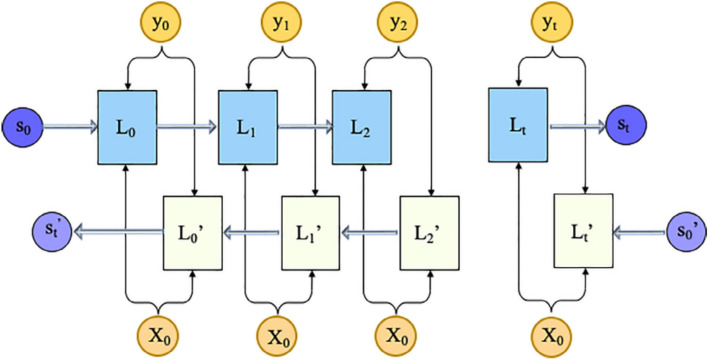 Figure 10
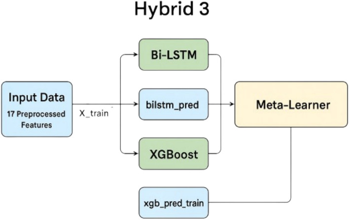 Figure 11
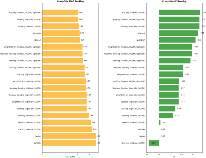 Figure 12
 Figure 13
 Figure 14
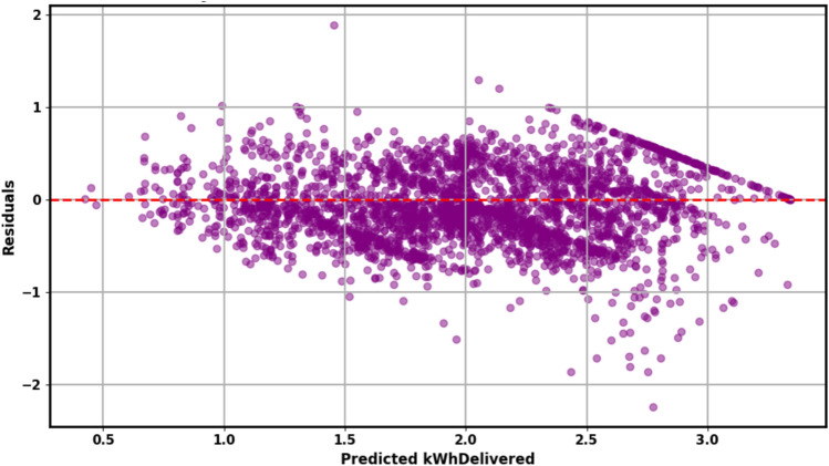 Figure 15
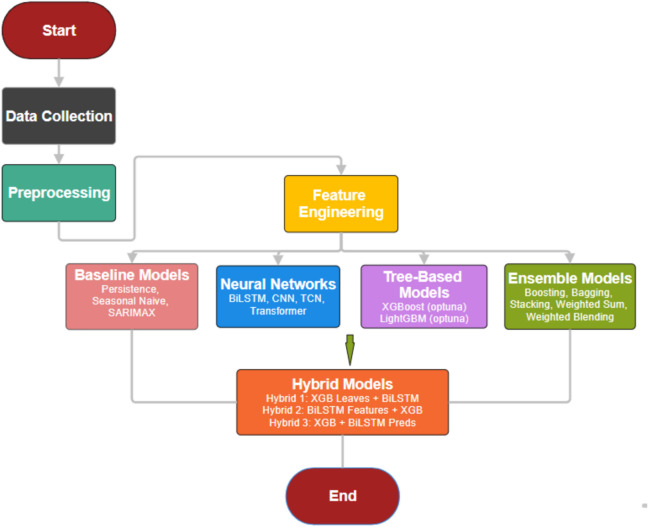 Figure 1
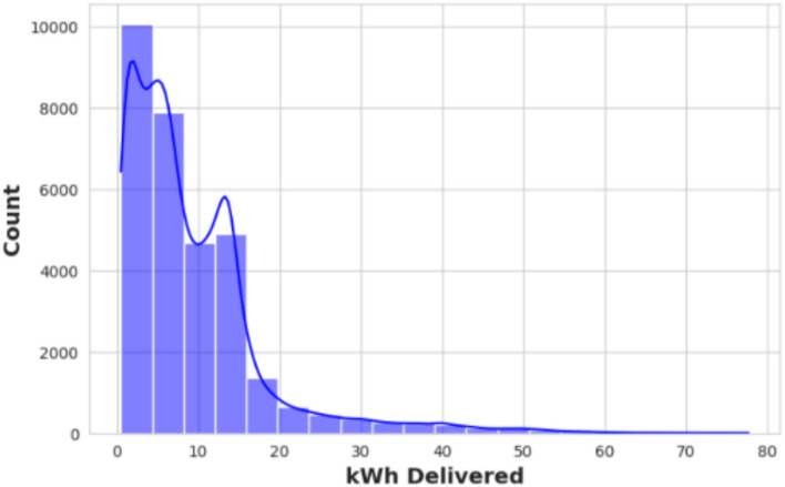 Figure 2
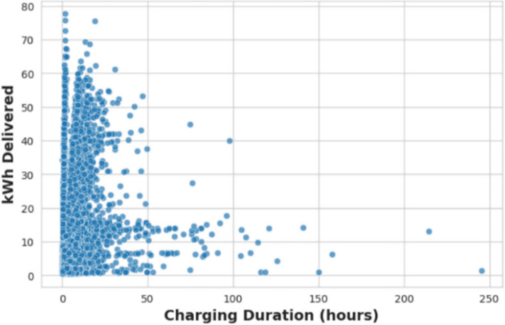 Figure 3
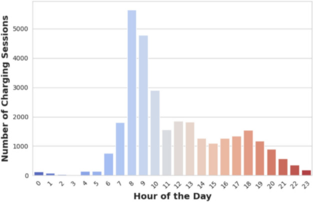 Figure 4
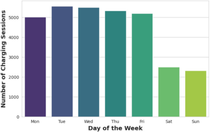 Figure 5
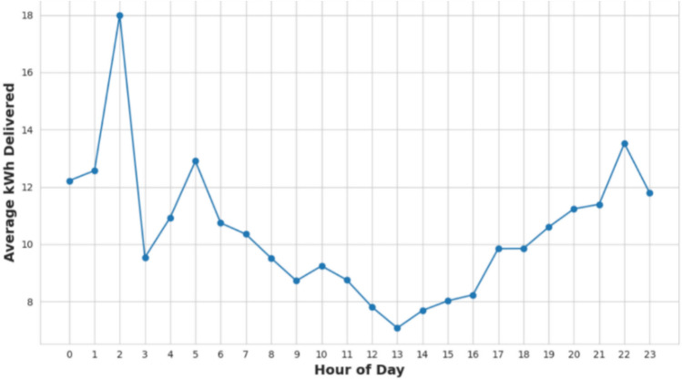 Figure 6
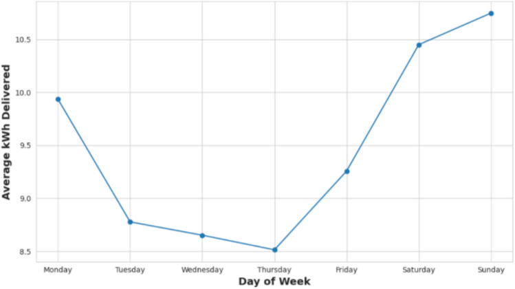 Figure 7
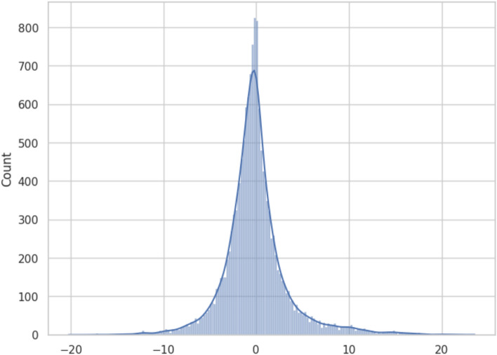 Figure 8
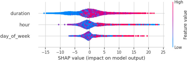 Figure 9
- —Suez Canal University
Peer Reviews
No public reviews on file for this paper yet. If you reviewed it on a platform where reviews are public (OpenReview, ICLR, NeurIPS, ICML), you can paste yours below so the community can read it here.
Videos
No videos yet. Explain this paper in a talk, walkthrough, or lecture? Add one.
Taxonomy
TopicsElectric Vehicles and Infrastructure · Energy Load and Power Forecasting · Smart Grid Energy Management
Introduction
Modern power systems integrate generation, transmission, and distribution to ensure efficient, reliable electricity delivery. These systems leverage advanced technologies to manage power flow, aiming for sustainable, cost-effective supply amid growing demand while minimizing environmental impact^1^. Accurate load forecasting is critical for grid operations, supporting short-term decisions (e.g., unit commitment, dispatch) and long-term planning (e.g., infrastructure expansion). Inaccurate forecasts risk increased costs, system instability, or blackouts^2^. The rapid rise in Electric Vehicle (EV) adoption has driven widespread charging station deployment, fueled by efforts to reduce fossil fuel reliance^3^. The European Union targets 750,000 public charging stations by 2025 (Alternative Fuels Infrastructure Regulation), the United States aims for 500,000 by 2030 (Bipartisan Infrastructure Law), and China leads with over 1.4 million public charging points, including high-speed chargers along major corridors. However, volatile EV charging demand, driven by unpredictable user behaviors, strains grid infrastructure^4^. Precise short-term, hourly, station-level load forecasting is essential for optimizing power consumption, resource allocation, and ensuring grid stability^5,6^. EV load forecasting methods include physically based and data-driven approaches. Physically based methods, like trip chain analysis^7^, Monte Carlo simulations^8^, and Markov decision processes^9^, are computationally intensive and less scalable^10^. Data-driven approaches, including statistical and AI-based techniques, are more efficient^11^. Statistical models, such as Autoregressive Integrated Moving Average (ARIMA) for EV loads^12^ or seasonal ARIMA for station profiles^13^, require minimal data but struggle with complex patterns. An adaptive Multilayer Perceptron (MLP) was developed for vehicle-to-grid scheduling^14^. Machine learning (ML) methods, like Support Vector Machines, Random Forests, and eXtreme Gradient Boosting (XGBoost)^15^, excel at nonlinear relationships but require extensive feature engineering and risk overfitting^16^. Deep learning (DL) approaches, including Convolutional Neural Networks (CNN), Long Short-Term Memory (LSTM), and Gated Recurrent Units, capture temporal dependencies^17^. Multivariate LSTM models with external factors (e.g., temperature, humidity) outperform univariate models^18^, while dynamic learning rates enhance forecasting at 15-min intervals^19^. Studies comparing LSTM, Bidirectional LSTM (BiLSTM), and CNN-LSTM highlight external factor impacts^4^. Advanced techniques, like adaptive proximal policy optimization^20^, Bayesian inference^21^, and hybrid Convolutional LSTM^22^, further improve accuracy.
Recent stacking-based ensembles have shown promise in energy forecasting by fusing diverse learners to mitigate overfitting and enhance generalization. For instance, a stack-based ensemble with meta-neural networks (SEFMNN) integrates ANN, RF, and SVM for solar irradiance prediction, achieving R^2^ > 0.99 while balancing computational efficiency^23^. Similarly, transformer-infused recurrent networks (TIR), combining BiLSTM encoders with GRU decoders and attention mechanisms, optimize short-term irradiance forecasts across regions like Munich and Texas, yielding RMSE as low as 0.014 with superior handling of meteorological variability^24^. Control-oriented advances, such as reinforcement learning (RL) frameworks like PPO and Meta-RL, enable dynamic adaptation in solar energy management, reducing operational costs by smoothing ramps and optimizing storage under uncertainty^25^. In contrast, our XGBoost-BiLSTM stacking (Hybrid 3) tailors these principles to EV charging dynamics, leveraging XGBoost as a meta-learner to ensemble tree-based nonlinearity with bidirectional temporal modeling—addressing EV-specific challenges like session volatility absent in solar data—while requiring less meteorological input than TIR or RL hybrids. Single ML or DL models are often inadequate for capturing both nonlinear patterns and temporal dependencies in EV charging data. XGBoost excels at modeling complex feature interactions but struggles with sequential dependencies, whereas BiLSTM effectively captures bidirectional temporal patterns but may miss intricate nonlinear relationships. Hybrid models combining ML and DL are increasingly recognized for addressing these shortcomings, yet their application to EV load forecasting remains underexplored.
A novel hybrid XGBoost–BiLSTM stacking ensemble (Hybrid 3) is proposed for short-term, hourly, station-level electric vehicle (EV) charging load forecasting. The model integrates XGBoost’s gradient-boosted decision trees with BiLSTM’s bidirectional temporal modeling, unified through an XGBoost meta-learner that learns optimal nonlinear combinations of the base learners’ predictions.
The proposed framework is evaluated using the Adaptive Charging Network (ACN) dataset, comprising 31,424 charging sessions collected from the Caltech mixed-use facility (April 2018–September 2021). Comprehensive benchmarking was performed against 24 baseline models spanning statistical (Persistence, Seasonal Naïve, SARIMAX, Prophet), machine learning (XGBoost, LightGBM), deep learning (CNN, TCN, Transformer, BiLSTM), and ensemble families (boosting, bagging, stacking, and weighted combinations).
On the cleaned dataset, Hybrid 3 achieved an MAE of 2.687 kWh and R^2^ = 0.6395, outperforming the standalone BiLSTM by 3.4%, and ranking among the top models while balancing accuracy, interpretability, and complexity. On the original (outlier-retained) dataset, Hybrid 3 maintained strong performance (MAE = 3.543 kWh, R^2^ = 0.5285), confirming robustness to noisy inputs.
Temporal robustness was validated through five-fold walk-forward validation, where Hybrid 3 achieved the lowest mean MAE (2.54 kWh) and highest mean R^2^ (0.63) across folds. One-way ANOVA (F = 1.624, p = 0.2073) showed no statistically significant differences among top models; however, the large effect size (η^2^ = 0.2062) indicated practical improvement.
Feature importance analysis identified charging duration (log-transformed) as the most influential predictor (importance = 0.376), emphasizing the dominant role of session length in determining delivered energy. The ablation study confirmed the critical contribution of each component: removing feature engineering (+ 13.7% MAE degradation), removing base learners (+ 18.8%), and removing the meta-learner (+ 29.2%), underscoring the stacking layer as the main performance driver.
External generalization was assessed using a cross-site synthetic dataset (~ 1.96 M sessions), where Hybrid 3 exhibited transferable but sensitivity-limited performance (MAE = 4.16 kWh, R^2^ = 0.01), while bagging ensembles achieved the best transfer accuracy (MAE = 3.08 kWh, R^2^ = 0.36). This study extends prior hybrid forecasting research (e.g., CNN-LSTM for smart building energy^26^) by introducing a stacking-enhanced XGBoost–BiLSTM framework specifically tailored for EV charging station load dynamics.
Major contributions
- Development of a hybrid XGBoost–BiLSTM stacking ensemble (Hybrid 3) that integrates gradient boosting and bidirectional sequence learning for short-term EV charging load forecasting.
- Design of a comprehensive benchmarking framework encompassing 24 baseline models across statistical, machine learning, deep learning, and ensemble families.
- Implementation of walk-forward validation to ensure temporal robustness and realistic performance assessment under non-stationary conditions.
- Execution of a detailed ablation study to quantify the contribution of each model component, highlighting the role of stacking and feature engineering in enhancing predictive performance.
- Integration of cross-site validation to evaluate model generalization and external validity under domain shift scenarios.
Overall, this work introduces a stacking-enhanced hybrid architecture tailored to EV charging dynamics, combining the interpretability of gradient boosting with the sequence modeling capability of BiLSTM. It establishes a robust foundation for data-driven EV energy forecasting, supporting effective charging network management and grid integration. Figure 1 presents the complete research methodology.Fig. 1. Research methodology.
Methodology
Dataset
This study utilizes the Adaptive Charging Network (ACN) dataset^27^, a comprehensive record of workplace EV charging sessions at a mixed-use parking facility on the Caltech campus. The dataset includes individual session characteristics and high-resolution time series data capturing power output for each charging unit. Key variables include EV arrival and departure timestamps, energy requested, and actual energy delivered (kWhDelivered) per session. The analysis covers data from 55 charging stations, primarily accessible to Caltech employees but also available for public use, including gym patrons. This mixed-use context makes the ACN dataset representative of both workplace and public charging patterns. The dataset spans 1329 days, from April 25, 2018, to September 13, 2021, comprising 31,424 charging sessions used for model training and evaluation. A summary of key data fields analyzed is presented in Table 1.Table 1ACN data field and description.FieldDescriptionData typeUnit / format_idUnique identifier for the database recordString–userInputsOptional user-provided metadata or session notesString / Null–sessionIDUnique identifier for the charging sessionString–stationIDIdentifier for the EV supply equipmentString–spaceIDIdentifier of the parking spaceString–siteIDIdentifier of the site where the session took placeString–clusterIDGroup identifier for related stations/sitesString–connectionTimeTimestamp when the vehicle was plugged inDatetimeISO 8601disconnectTimeTimestamp when the vehicle was unpluggedDatetimeISO 8601kWhDeliveredTotal energy delivered during the sessionFloatkWhdoneChargingTimeTimestamp when charging completedDatetimeISO 8601timezoneLocal timezone of the siteStringOlson identifieruserIDAnonymized identifier for the userString / Null–
Dataset analysis
To gain a clearer understanding of the characteristics within these datasets, a concise exploratory analysis was performed. Figure 2 presents a histogram depicting the distribution of energy delivered during individual charging sessions, overlaid with a kernel density estimate (KDE). The distribution exhibits a marked right skew, with frequencies sharply decreasing as the amount of energy delivered increases. This suggests that most charging sessions involve relatively small energy transfers. Notably, there is an uptick in frequencies between 2 and 10 kWh, implying that many users prefer shorter or partial charges rather than fully charging their vehicles. The long tail of the distribution reflects a minority of sessions requiring substantially greater energy.Fig. 2. Distribution of delivered energy.
Figure 3 illustrates the relationship between charging duration and the amount of energy dispensed. The majority of charging events are concentrated in the shorter duration range, between 0 and 50 h, with a broad spectrum of energy amounts delivered. The plot reveals a distinct right-skewed pattern, indicating the presence of outliers characterized by exceptionally long charging times coupled with minimal additional energy provided. This pattern suggests that while most users complete their charging relatively swiftly, a few engage in extended sessions. Such prolonged charging intervals with low energy output may point to irregularities or inefficiencies within the charging process.Fig. 3. Charging duration vs. energy delivered.
The distribution of charging sessions across different times of the day is depicted in Fig. 4. A pronounced surge in activity occurs between 8 and 10 AM, indicating that many users prefer to recharge their vehicles during the morning hours. After this peak, charging activity tends to stabilize through the afternoon and evening, gradually diminishing late at night and in the early morning. The notably lower charging frequencies during these off-peak hours likely reflect reduced demand or decreased vehicle usage during these periods.Fig. 4. Daily charging sessions spread.
Figure 5 displays the frequency of charging sessions by day of the week. The bar chart reveals higher charging activity throughout the workweek, Monday to Friday, with a peak occurring on Tuesday and Wednesday. In contrast, weekend days exhibit a significant decline in charging sessions. This pattern suggests that the typical workweek schedule strongly influences charging behavior, with users predominantly charging their vehicles during weekdays. Figure 6 illustrates the average charging demand by hour, based on the ACN dataset. The graph indicates a peak demand occurring at 2 AM, while the lowest demand is observed at 1 PM.Fig. 5. Charging sessions by day of the week.Fig. 6. Average charging demand by hour of day.
Figure 7 features a line graph portraying average daily charging demand across the week. The data shows a downward trend in demand from Monday through Thursday, reaching its lowest point on Thursday. Demand subsequently rises on Friday, culminating in the highest levels observed on Sunday. These patterns underscore the variability in charging behavior throughout the week and highlight the weekend as a period of increased energy needs. Such information is critical for effective load forecasting and the strategic placement of charging infrastructure to manage peak demand periods.Fig. 7. Average charging demand by day of week.
Figure 8 visualizes the residuals, or prediction errors, of the load forecasting model. The residuals are predominantly centered around zero, indicating that the model’s predictions are largely unbiased. The distribution’s shape suggests that most errors are small; nonetheless, occasional larger deviations are evident, corresponding to under- or overestimations. Overall, the model’s residuals appear well-behaved, contributing to confidence in its predictive reliability. The SHAP summary plot (Fig. 9) provides a model-agnostic interpretation of feature impacts, corroborating the Gini-based importance rankings in Table 9. It confirms that charging_duration is the overwhelmingly dominant predictor of EV charging load, with longer sessions exhibiting a strong positive correlation with higher energy delivery. This primacy of session-level features over temporal ones like hour and day_of_week provides a crucial explanation for the model performance patterns observed throughout this study. The reliance on charging_duration elucidates why tree-based models like XGBoost and LightGBM performed robustly, as they excel at capturing such strong, non-linear, tabular relationships. Furthermore, it explains the high weight assigned to the xgb_pred component within the Hybrid 3 ensemble (Table 9), as the meta-learner optimally leverages XGBoost’s strength in modeling this key feature. This finding also offers a post-hoc interpretation of the ANOVA results (Table 12), which indicated no statistically significant difference in performance among the top models. The dominance of a single feature suggests that any model capable of effectively learning the charging_duration relationship will achieve competitive accuracy, thereby converging on similar performance levels and resulting in a non-significant ANOVA p-value. While this alignment with domain knowledge—where longer sessions logically transfer more energy—validates the model’s logic, it also highlights a potential limitation. The model’s performance is heavily contingent on accurate duration data, which may not always be available for long-horizon forecasts. Furthermore, the overshadowing of temporal features indicates that the current models may be less effective at predicting load variations driven purely by time-of-use patterns or external factors like grid events, pointing to a area for future work where incorporating additional contextual variables could yield improvements.Fig. 8. Residual distribution of the load forecasting model.Fig. 9SHAP value.
Preprocessing
All models were trained with a fixed random seed (seed = 42) to ensure full reproducibility. The ACN–Caltech site dataset was randomly split into 80% for training and 20% for testing without shuffling, maintaining temporal consistency and representative sampling. The electric vehicle (EV) charging session dataset from the ACNPortal was preprocessed to enhance its suitability for predicting energy consumption (kWhDelivered), focusing on data cleaning, feature engineering, outlier management, and missing value handling to support robust model performance. Initial cleaning removed irrelevant identifier columns (_id, sessionID, stationID, spaceID, siteID, clusterID, userID) to streamline analysis, while datetime columns (connectionTime, disconnectTime, doneChargingTime) were converted to a timezone-naive format to ensure consistent temporal processing. Feature engineering enriched the dataset with temporal and derived variables: hour (0–23), day_of_week (0–6), and month (1–12) were extracted from connectionTime; a binary is_weekend feature (1 for Saturday/Sunday, 0 otherwise) and a season feature (0–3, mapping months to Winter, Spring, Summer, Fall) were created to capture weekly and seasonal patterns. Cyclical features (hour_sin, hour_cos) modeled the 24-h cycle, while day_of_year (1–365) and week_of_year (1–52) represented annual and weekly trends. A binary is_holiday feature (1 for December/January, 0 otherwise) accounted for holiday effects. Charging-related features included duration (disconnectTime minus connectionTime, in hours) and charging_duration (doneChargingTime minus connectionTime, in hours), with charging_duration_log applied to mitigate skewness, as confirmed by a skewness value of 1.24 (Table 2). Interaction terms (hour_charging_interaction, weekend_charging_interaction) and lagged features (lag_1_log, lag_2_log, lag_3_log) based on log-transformed duration, along with rolling_mean_3_log and rolling_mean_5_log, captured historical patterns, with non-numeric values coerced to NaN and converted to float64.Table 2. Feature skewness analysis.FeatureSkewness valuehour0.87day_of_week0.31month − 0.04season0.00duration0.60charging_duration1.24charging_duration_log0.70hour_sin − 0.66hour_cos1.47day_of_year − 0.03week_of_year − 0.02is_holiday1.46lag_1_log − 0.18lag_2_log − 0.19lag_3_log − 0.19rolling_mean_3_log − 0.33rolling_mean_5_log − 0.38kWhDelivered (Target)1.09Skewness measures for all features and the target variable. Values > 1 or < -1 indicate significant skewness requiring transformation.
Outlier management employed the Interquartile Range (IQR) method, calculating Q1 and Q3 for duration, charging_duration, and kWhDelivered, defining the IQR as Q3 minus Q1, and capping values between Q1—1.5 × IQR and Q3 + 1.5 × IQR to reduce the impact of extreme values. A copy of the original dataset (df_original) was preserved for comparative analysis. Missing values, arising from feature engineering or lags, were removed, and the original dataset was aligned to the cleaned dataset’s indices. Table 2 (Feature Skewness Analysis) guided transformations, revealing significant skewness (> 1 or < -1) for charging_duration (1.24), hour_cos (1.47), and is_holiday (1.46), and moderate skewness for kWhDelivered (1.09), prompting a log transform for the target to improve model fit. A data leakage check confirmed no identical rows between training and test sets by converting data to tuples and checking set intersections, preserving temporal integrity. The preprocessed dataset, comprising 17 features (hour, day_of_week, month, season, duration, charging_duration, charging_duration_log, hour_sin, hour_cos, day_of_year, week_of_year, is_holiday, lag_1_log, lag_2_log, lag_3_log, rolling_mean_3_log, rolling_mean_5_log) and kWhDelivered as the target, was thus optimized for training and evaluating machine learning, deep learning, and ensemble models.
Models
XGBoost (eXtreme Gradient Boosting)
The XGBoost algorithm, introduced by Tianqi Chen in 2016, is a powerful decision tree–based ensemble method that utilizes the boosting technique to improve predictive performance^28^. The XGBoost algorithm addresses these challenges by incorporating enhancements including tree pruning, parallel processing, and the introduction of regularization terms, thereby improving the overall robustness and efficiency of the model.
BiLSTM
BiLSTM networks comprise two distinct LSTM layers arranged to process sequential data in opposite temporal directions. Specifically, one layer analyzes the input sequence in the forward direction, while the other simultaneously traverses it in reverse, thereby enabling the model to capture contextual information from both past and future states within the sequence^29^. These two outputs are then combined to produce the final prediction. Unlike a standard LSTM, which analyzes time-dependent data in only one direction, BiLSTM incorporates this additional reverse pass to capture patterns and dependencies that may be overlooked when considering the sequence in a single direction. The architecture of the BiLSTM approach is shown in Fig. 10, where Li denotes the forward LSTM layer, Li represents the backward LSTM layer, and s and s′ correspond to the time series information propagated through the respective LSTM cells.Fig. 10. Schematic diagram of BiLSTM.
XGBoost and Bi-LSTM (Hybrid 3 model)
The Hybrid 3 model combines the strengths of XGBoost and Bidirectional Long Short-Term Memory (BiLSTM) networks to enhance the prediction of energy consumption (kWhDelivered) in the electric vehicle (EV) charging session dataset. BiLSTM excels at capturing temporal dependencies and sequential patterns in time-series data, leveraging its bidirectional architecture to model relationships in both forward and backward directions across the 17 preprocessed features (e.g., hour, charging_duration_log, lag_1_log). Conversely, XGBoost is adept at handling structured data, capturing complex nonlinear interactions among features through gradient boosting and tree-based learning. By integrating these models, Hybrid 3 aims to combine BiLSTM’s sequential modeling capabilities with XGBoost’s robust feature interaction modeling to achieve superior predictive accuracy compared to standalone models.
The Hybrid 3 model was implemented as a stacking ensemble. First, predictions were generated independently from two base models: (1) an optimized XGBoost model, tuned using Optuna with parameters such as n_estimators, max_depth, and learning_rate trained on the scaled feature set (X_train_scaled); and (2) a BiLSTM model with three bidirectional LSTM layers (128, 64, and 64 units, respectively), regularized with L2 regularization (0.0001) and dropout (0.07), trained on the 3D input (X_train_lstm) reshaped to include a time-step dimension. These predictions (xgb_pred_train, bilstm_pred_train for training; xgb_pred_test, bilstm_pred_test for testing) were stacked column-wise to form a meta-feature matrix (X_meta_train, X_meta_test). A meta-learner, implemented as an XGBoost model with default parameters and a random seed of 42, was trained on X_meta_train to predict the target (y_train), effectively learning to weigh the contributions of the base models’ predictions. The meta-learner then generated final predictions on X_meta_test for evaluation.
This stacking approach leverages BiLSTM’s ability to model temporal dynamics, such as diurnal and seasonal charging patterns, while incorporating XGBoost’s strength in capturing feature interactions, such as those between hour_charging_interaction and charging_duration_log. The model was trained on the preprocessed dataset and evaluated using metrics including Mean Absolute Error (MAE), Mean Squared Error (MSE), Root Mean Squared Error (RMSE), and R^2^, with performance assessed on both cleaned and original (pre-outlier-capping) datasets to ensure robustness The training and testing times were recorded as hybrid 3_training_time and hybrid 3_testing_time, respectively, to assess computational efficiency. This hybrid framework was designed to mitigate the limitations of individual models, delivering more reliable and precise predictions for EV charging energy demand forecasting.
Figure 11 illustrates the architecture of the proposed Hybrid 3 model, which integrates an optimized XGBoost regressor and a BiLSTM neural network within a stacking ensemble framework for short-term EV charging load forecasting.Fig. 11. Architecture of the hybrid 3 (XGBoost–BiLSTM) stacking ensemble model.
In the first stage, the preprocessed feature set is independently input into two base learners:
- XGBoost, which captures nonlinear relationships and feature interactions, and
- BiLSTM, which models temporal dependencies and sequential patterns across charging sessions.
Each base model generates preliminary predictions that are concatenated to form a meta-feature matrix. This matrix is then used to train an XGBoost meta-learner, which learns optimal weights for combining the base models’ outputs to generate the final prediction.
This hybrid design leverages BiLSTM’s ability to model time-series dynamics alongside XGBoost’s strength in structured feature learning, thereby improving both accuracy and robustness in EV energy demand forecasting.
Other baseline models
This study evaluates 24 baseline models spanning statistical, machine learning, deep learning, and ensemble categories to provide comprehensive benchmarking against the proposed Hybrid 3 model. All baseline models were implemented with architectures and hyperparameters specified in Table 3, ensuring fair comparison across diverse methodologies.Table 3. Hyperparameter search ranges and fixed values.ModelHyperparameterRange/ValueNotesXGBoostn_estimators1000–3000 (step 200)Number of boosting roundsmax_depth4–8Maximum tree depthlearning_rate0.005–0.1 (log scale)Step size shrinkagesubsample0.7–0.95Subsample ratio of the training instancescolsample_bytree0.7–0.95Subsample ratio of columns per treecolsample_bylevel0.7–0.95Subsample ratio of columns per levelgamma0–0.3Minimum loss reduction for splitmin_child_weight1–10Minimum sum of instance weightreg_alpha0–5L1 regularization termreg_lambda0.5–5L2 regularization termLightGBMn_estimators10–100 (step 10)Number of boosting iterationsmax_depth2–5Maximum tree depthlearning_rate0.1–0.3 (log scale)Step size shrinkagenum_leaves10–50Maximum number of leaves per treesubsample0.5–0.9Subsample ratio of the training instancescolsample_bytree0.5–0.9Subsample ratio of columns per treemin_child_samples20–100Minimum number of data in a leafreg_alpha0–5L1 regularization termreg_lambda0.5–5L2 regularization termsubsample_freq1–10Frequency of subsampleBiLSTMunits128, 64, 64Units per LSTM layer (fixed architecture)num_layers3Number of LSTM layers (fixed)learning_rate0.0005Fixed learning rate for AdamWbatch_size128Fixed batch sizedropout0.07Dropout rate (fixed)l2_regularization0.0001L2 regularization (fixed)CNNfilters64, 32Filters per convolutional layer (fixed)kernel_size3Kernel size (fixed)learning_rate0.001Fixed learning rate for AdamWbatch_size128Fixed batch sizeTCNnb_filters64Number of filters (fixed)kernel_size3Kernel size (fixed)dilations[1, 2, 4]Dilation rates (fixed)learning_rate0.001Fixed learning rate for AdamWbatch_size128Fixed batch sizeTransformernum_heads4Number of attention heads (fixed)key_dim64Dimension of attention keys (fixed)num_layers2Number of attention layers (fixed)learning_rate0.001Fixed learning rate for AdamWbatch_size128Fixed batch sizeSARIMAXp (AR order)1Autoregressive order (fixed)d (differencing)1Differencing order (fixed)q (MA order)1Moving average order (fixed)seasonal_order(1, 1, 1, 24)Seasonal order (fixed, 24-h period)Prophetyearly_seasonalityTrueFixed settingweekly_seasonalityTrueFixed settingdaily_seasonalityTrueFixed settingHyperparameter ranges for XGBoost and LightGBM were tuned using Optuna with TimeSeriesSplit (3 folds for XGBoost, variable for LightGBM). Neural network models (BiLSTM, CNN, TCN, Transformer) use fixed architectures with specified hyperparameters, optimized via early stopping and learning rate reduction. SARIMAX and Prophet use fixed configurations.
Statistical Baselines: Four traditional time series models were implemented as performance baselines. The Persistence model uses the previous observation as the forecast (y_t = y_{t-1}), serving as a naive benchmark. Seasonal Naïve applies 24-h periodicity forecasting (y_t = y_{t-24}), capturing diurnal patterns. SARIMAX employs an autoregressive integrated moving average model with exogenous variables using order (1,1,1) and seasonal order (1,1,1,24) to account for hourly patterns. Prophet implements additive time series modeling with configurable yearly, weekly, and daily seasonality components, incorporating all 17 engineered features as regressors.
Deep Learning Baselines: Three advanced neural architectures complement the BiLSTM model. The Convolutional Neural Network (CNN) uses two convolutional layers (64 and 32 filters, kernel size 3) followed by max pooling and dense layers, capturing local temporal patterns through 1D convolutions. The Temporal Convolutional Network (TCN) implements dilated convolutions with 64 filters, kernel size 3, and dilation rates^1,2,4^ to model long-range dependencies efficiently. The Transformer model employs two multi-head attention layers (4 heads, key dimension 64) with layer normalization and residual connections, leveraging self-attention mechanisms to capture global temporal dependencies across the input sequence.
Machine Learning Baselines: Two gradient boosting frameworks provide robust nonlinear modeling. XGBoost (eXtreme Gradient Boosting) uses tree-based ensemble learning with hyperparameters optimized via Optuna (Table 4), incorporating early stopping and L1/L2 regularization for robustness. LightGBM (Light Gradient Boosting Machine) employs histogram-based learning with leaf-wise tree growth, also tuned via Optuna, offering superior computational efficiency through gradient-based one-side sampling.Table 4. Optimal hyperparameters for XGBoost and LightGBM.ParameterXGBoostLightGBMn_estimators1400100max_depth64learning_rate0.0072970.131602subsample0.8106290.767120colsample_bytree0.9051820.832741colsample_bylevel0.749766–gamma0.177765–min_child_weight6–min_child_samples–38reg_alpha0.5252834.389436reg_lambda3.9784451.668866subsample_freq–9
Ensemble Baselines: Twelve ensemble methods systematically combine base learners to explore integration strategies. Boosting ensembles implement sequential residual learning, where each model corrects the predecessor’s errors through weighted averaging (equal weights). Bagging ensembles use bootstrap aggregation with 10 estimators trained in parallel, reducing variance through averaging. Stacking ensembles employ meta-learning architectures where base model predictions serve as features for a final XGBoost meta-learner. Weighted combinations apply optimized linear combinations with fixed weights (0.6/0.4 for two models, 0.4/0.3/0.3 for three models), representing both weighted sum and blending approaches.
Alternative Hybrid Baselines: Two additional hybrid architectures provide comparative analysis of XGBoost-BiLSTM integration strategies. Hybrid 1 implements feature concatenation, where XGBoost’s tree structure outputs are stacked with original features to form an expanded input for the BiLSTM network, creating a 18-dimensional feature space. Hybrid 2 uses sequential prediction fusion, extracting latent representations from BiLSTM’s intermediate layers (excluding final dense layers) as sequential features for subsequent XGBoost regression, effectively transferring temporal knowledge through dimensionality-reduced embeddings.
All baseline models were evaluated using the comprehensive framework outlined in Sect. “Evaluation metrics”, with performance metrics computed on both cleaned and original datasets to assess robustness. Hyperparameter optimization employed TimeSeriesSplit cross-validation (3 folds for tree-based models), early stopping for neural networks, and fixed configurations for statistical models, ensuring methodological consistency across the 25-model comparison.
The following Table 3 outlines the hyperparameter ranges or fixed values used for tuning and training the models in this study, optimized for forecasting EV charging load (kWhDelivered) using the ACN dataset.
Table 4 below lists the best hyperparameters for the XGBoost and LightGBM models, obtained through Optuna optimization with TimeSeriesSplit.
External validation dataset
This dataset comprises 1,965,239 simulated charging sessions representing a distinct, generic EVCS site, designed to assess domain-shift effects in a controlled yet realistic setting.
The dataset was preprocessed to align with the ACN schema. Energy delivery values (kWhDelivered) were clipped to a realistic EV range (0–100 kWh) to remove synthetic outliers, and temporal features (hour, day_of_week, month, season, is_holiday, is_weekend) were reconstructed from connection timestamps. Missing environmental context was addressed by generating synthetic meteorological variables—temperature (T ~ N(20 C, 5)) and humidity (H ~ N(60%, 15))—using seeded Gaussian noise (seed = 42) for reproducibility. A synthetic timeline was constructed by combining day_of_week and connectionTime_decimal to form a continuous chronological sequence spanning multiple simulated years.
Descriptive statistics of the cross-site dataset prior to preprocessing are summarized in Table 5. The distribution of kWhDelivered exhibits a right-skewed profile typical of partial EV charges (mean = 9.44 kWh, SD = 5.70), while session durations vary widely (mean = 3.80 h). These characteristics confirm that the dataset adequately reflects heterogeneous charging behaviors necessary for robust cross-site evaluation. Results from this external validation are reported in Sect. “External validation results”.Table 5. Descriptive statistics of the cross-site dataset (pre-processing).StatisticconnectionTime_decimalcharging_durationkWhDeliveredday_of_weekCount1,965,2391,965,2391,965,2391,965,239Mean14.493.809.4414,800.03Std6.433.395.708,531.91Min0.000.000.001.0025%14.251.444.877,424.0050%16.172.559.1714,793.0075%18.045.4413.5722,198.00Max24.0039.4162.5429,600.00
Computational environment
All computational experiments were performed on a system utilizing two NVIDIA Tesla T4 GPUs (16 GB VRAM each) with CUDA Version 12.6 and an x86_64 CPU. Deep learning models (BiLSTM, CNN, Transformer) were accelerated using TensorFlow and with GPU support, while ensemble methods (XGBoost, LightGBM) primarily leveraged CPU resources.
Evaluation metrics
To evaluate the performance of the proposed models for forecasting energy delivered (kWhDelivered) in EV charging sessions, we employed a suite of standard regression metrics: Mean Absolute Error (MAE), Mean Squared Error (MSE), Root Mean Squared Error (RMSE), and the Coefficient of Determination (R^2^). These metrics were calculated for both training and testing datasets, with evaluations conducted on both the cleaned dataset (after outlier removal and preprocessing) and the original dataset (before outlier removal) to assess model robustness. Additionally, walk-forward validation and statistical testing were applied to ensure robust and reliable performance comparisons across models. Below, we describe each metric, its mathematical formulation, its relevance to the task, and the evaluation methodology.
Mean squared error (MSE)
The MSE quantifies the average of the squared deviations between the observed and predicted values. A lower MSE indicates superior predictive accuracy, with an ideal value of zero representing a perfect correspondence between the actual and forecasted data.
\documentclass[12pt]{minimal} \usepackage{amsmath} \usepackage{wasysym} \usepackage{amsfonts} \usepackage{amssymb} \usepackage{amsbsy} \usepackage{mathrsfs} \usepackage{upgreek} \setlength{\oddsidemargin}{-69pt} \begin{document}$$MSE=\frac{1}{n}\sum_{i=1}^{n}{\left({y}_{i}-{\widehat{y}}_{i}\right)}^{2}$$\end{document}where, n denotes the total number of observations considered, \documentclass[12pt]{minimal} \usepackage{amsmath} \usepackage{wasysym} \usepackage{amsfonts} \usepackage{amssymb} \usepackage{amsbsy} \usepackage{mathrsfs} \usepackage{upgreek} \setlength{\oddsidemargin}{-69pt} \begin{document}$${\widehat{{\varvec{y}}}}_{{\varvec{i}}}$$\end{document} represents the predicted or forecasted value, and \documentclass[12pt]{minimal} \usepackage{amsmath} \usepackage{wasysym} \usepackage{amsfonts} \usepackage{amssymb} \usepackage{amsbsy} \usepackage{mathrsfs} \usepackage{upgreek} \setlength{\oddsidemargin}{-69pt} \begin{document}$${{\varvec{y}}}_{{\varvec{i}}}$$\end{document} corresponds to the true or observed value.
Root mean squared error (RMSE)
The RMSE is defined as the square root of the MSE and possesses the advantage of being expressed in the same units as the target variable, thereby facilitating interpretability.
\documentclass[12pt]{minimal} \usepackage{amsmath} \usepackage{wasysym} \usepackage{amsfonts} \usepackage{amssymb} \usepackage{amsbsy} \usepackage{mathrsfs} \usepackage{upgreek} \setlength{\oddsidemargin}{-69pt} \begin{document}$$RMSE=\sqrt{\frac{1}{n}\sum_{i=1}^{n}{\left({y}_{i}-{\widehat{y}}_{i}\right)}^{2}}$$\end{document}Mean absolute error (MAE)
This metric represents the average of the absolute deviations between the observed values and their corresponding forecasts, providing a direct measure of prediction accuracy in terms of magnitude of errors.
\documentclass[12pt]{minimal} \usepackage{amsmath} \usepackage{wasysym} \usepackage{amsfonts} \usepackage{amssymb} \usepackage{amsbsy} \usepackage{mathrsfs} \usepackage{upgreek} \setlength{\oddsidemargin}{-69pt} \begin{document}$$MAE=\frac{1}{n}\sum_{i=1}^{n}\left|{y}_{i}-{\widehat{y}}_{i}\right|$$\end{document}Coefficient of determination (R2)
The coefficient of determination, commonly referred to as R-squared (R^2^), evaluates the goodness-of-fit of a predictive model by quantifying the proportion of variance in the observed data that is explained by the model’s predictions. This metric ranges between 0 and 1, where a value of 0 indicates that the model fails to capture the underlying data patterns, reflecting poor fit, and a value of 1 denotes perfect prediction accuracy with no deviation from the actual observations.
\documentclass[12pt]{minimal} \usepackage{amsmath} \usepackage{wasysym} \usepackage{amsfonts} \usepackage{amssymb} \usepackage{amsbsy} \usepackage{mathrsfs} \usepackage{upgreek} \setlength{\oddsidemargin}{-69pt} \begin{document}$${R}^{2}=1-\frac{\sum_{i=1}^{M}{\left({\widehat{y}}_{i}-{y}_{i}\right)}^{2}}{\sum_{1=1}^{M}{\left(\overline{{y }_{i}}-{y}_{i}\right)}^{2}}$$\end{document}Walk-forward validation
To further validate model performance in a time-series context, walk-forward validation was conducted using a fivefold TimeSeriesSplit. This approach simulates rolling forecasts by training on progressively larger subsets of the data and testing on subsequent time periods, ensuring temporal consistency. The top-performing models (XGBoost, LightGBM, BiLSTM, Stacking (XGBoost, BiLSTM, LightGBM), and Hybrid 3 (XGBoost, BiLSTM)) were evaluated, with metrics (MAE, MSE, RMSE, R^2^) calculated for each fold. The mean and standard deviation of these metrics across folds were reported to assess model stability and generalization. Walk-forward validation is particularly relevant for EV charging forecasting, as it reflects the dynamic nature of charging session data over time.
Statistical testing
To determine whether performance differences between models were statistically significant, a one-way ANOVA test was performed on the MAE values from walk-forward validation. The ANOVA test evaluates the null hypothesis that all models have the same mean MAE, with a p-value threshold of 0.05. The effect size ( \documentclass[12pt]{minimal} \usepackage{amsmath} \usepackage{wasysym} \usepackage{amsfonts} \usepackage{amssymb} \usepackage{amsbsy} \usepackage{mathrsfs} \usepackage{upgreek} \setlength{\oddsidemargin}{-69pt} \begin{document}$${\upeta }^{2}$$\end{document} ) was calculated to quantify the magnitude of differences:
\documentclass[12pt]{minimal} \usepackage{amsmath} \usepackage{wasysym} \usepackage{amsfonts} \usepackage{amssymb} \usepackage{amsbsy} \usepackage{mathrsfs} \usepackage{upgreek} \setlength{\oddsidemargin}{-69pt} \begin{document}$${\upeta }^{2}=\frac{F\cdot (k-1)}{F\cdot \left(k-1\right)+n}$$\end{document}where \documentclass[12pt]{minimal} \usepackage{amsmath} \usepackage{wasysym} \usepackage{amsfonts} \usepackage{amssymb} \usepackage{amsbsy} \usepackage{mathrsfs} \usepackage{upgreek} \setlength{\oddsidemargin}{-69pt} \begin{document}$$F$$\end{document} is the ANOVA F-statistic, \documentclass[12pt]{minimal} \usepackage{amsmath} \usepackage{wasysym} \usepackage{amsfonts} \usepackage{amssymb} \usepackage{amsbsy} \usepackage{mathrsfs} \usepackage{upgreek} \setlength{\oddsidemargin}{-69pt} \begin{document}$$k$$\end{document} is the number of models, and \documentclass[12pt]{minimal} \usepackage{amsmath} \usepackage{wasysym} \usepackage{amsfonts} \usepackage{amssymb} \usepackage{amsbsy} \usepackage{mathrsfs} \usepackage{upgreek} \setlength{\oddsidemargin}{-69pt} \begin{document}$$n$$\end{document} is the total number of observations. An \documentclass[12pt]{minimal} \usepackage{amsmath} \usepackage{wasysym} \usepackage{amsfonts} \usepackage{amssymb} \usepackage{amsbsy} \usepackage{mathrsfs} \usepackage{upgreek} \setlength{\oddsidemargin}{-69pt} \begin{document}$${\upeta }^{2}$$\end{document} value below 0.06 indicates a small effect, 0.06–0.14 a medium effect, and above 0.14 a large effect. Additionally, 95% confidence intervals for MAE were computed for each model using the t-distribution to assess the precision of performance estimates. These statistical analyses ensure robust comparisons and guide model selection.
Computational efficiency
In addition to predictive performance, computational efficiency was evaluated by measuring tuning time, training time, and testing time for each model. These metrics, recorded in seconds, are critical for practical deployment in real-time EV charging systems, where low latency is essential.
The computational efficiency of the models, as detailed in Table 6, is a critical factor for their practical deployment in real-time EV charging systems, where low latency is essential for dynamic load management. Training and testing times, measured in seconds, were recorded for both cleaned and original datasets, with tuning times reported for XGBoost and LightGBM via Optuna. The results reveal significant variability across models, reflecting differences in algorithmic complexity and ensemble strategies.Table 6. Training and testing times of models.ModelTraining time (s)Testing time (s)SARIMAX392.720.30Prophet3.122.27BiLSTM103.780.47CNN21.170.42TCN24.820.59Transformer44.290.90XGBoost1.900.03LightGBM0.100.01Boosting (XGBoost, BiLSTM)2.290.00Bagging (XGBoost, BiLSTM)21.411.81Stacking (XGBoost, BiLSTM)517.293.71Boosting (XGBoost, BiLSTM, LightGBM)0.040.00Bagging (XGBoost, BiLSTM, LightGBM)1.020.36Stacking (XGBoost, BiLSTM, LightGBM)531.563.85Bagging (LightGBM, BiLSTM)1.040.41Stacking (LightGBM, BiLSTM)536.244.20Hybrid 1 (XGBoost, BiLSTM)1471.2146.70Hybrid 2 (XGBoost, BiLSTM)6.770.18Hybrid 3 (XGBoost, BiLSTM)2.520.01
LightGBM stands out as the most computationally efficient model, with a training time of 0.10 s and a testing time of 0.01 s, making it highly suitable for scenarios requiring rapid updates. XGBoost follows with a training time of 1.90 s and a testing time of 0.03 s, benefiting from its optimized tree-boosting implementation. Among hybrid and ensemble models, Hybrid 3 (XGBoost, BiLSTM) achieves a commendable balance, with a training time of 2.52 s and a testing time of 0.01 s, closely aligning with the efficiency of standalone XGBoost. This efficiency is attributed to the stacking ensemble’s use of precomputed base model predictions, reducing redundant computations during testing.
In contrast, more complex ensemble models exhibit higher computational demands. Stacking (XGBoost, BiLSTM, LightGBM) requires 531.56 s for training and 3.85 s for testing, reflecting the overhead of training multiple base models and a meta-learner. Hybrid 1 (XGBoost, BiLSTM) is the least efficient, with a training time of 1471.21 s and a testing time of 46.70 s, likely due to its unique implementation or resource-intensive optimization. Statistical models like SARIMAX (392.72 s training, 0.30 s testing) and deep learning models like BiLSTM (103.78 s training, 0.47 s testing) also show higher training times, though their testing times remain low, suitable for inference.
The low testing times across most models (e.g., 0.00–0.90 s) suggest feasibility for real-time applications, with Hybrid 3’s 0.01-s testing time indicating potential for near-instantaneous predictions. However, training times for complex models (e.g., Stacking, Hybrid 1) highlight the need for offline or periodic retraining rather than on-the-fly updates. The efficiency of Hybrid 3, combined with its competitive predictive performance (MAE of 2.6870 kWh on cleaned data), positions it as a practical choice for EV charging load forecasting, especially when balanced against accuracy requirements. Future work could explore parallelization or lightweight variants to further reduce training times for scalable deployment.
Results and discussion
This section presents a comprehensive evaluation of the models developed for forecasting energy delivered (kWhDelivered) at electric vehicle charging stations (EVCS), utilizing the Adaptive Charging Network (ACN) dataset. The analysis compares model performance on cleaned and original datasets using Mean Absolute Error (MAE), Mean Squared Error (MSE), Root Mean Squared Error (RMSE), and the Coefficient of Determination (R^2^). Subsequent subsections assess temporal robustness through walk-forward validation, statistical significance via ANOVA, and computational efficiency for practical deployment. The discussion concludes with implications, recommendations, and limitations, drawing on data from Tables 7, 8, 9, 10, 11, 12, 13 and supplementary analyses.Table 7. Models performance on cleaned data.ModelSplitMAE (kWh)MSE (kW \documentclass[12pt]{minimal} \usepackage{amsmath} \usepackage{wasysym} \usepackage{amsfonts} \usepackage{amssymb} \usepackage{amsbsy} \usepackage{mathrsfs} \usepackage{upgreek} \setlength{\oddsidemargin}{-69pt} \begin{document}$${h}^{2})$$\end{document} RMSE (kWh)R^2^PersistenceTrain7.658899.96519.9983 − 0.8929Test6.702985.91189.2689 − 0.9525Seasonal NaïveTrain7.7371101.876310.0934 − 0.9291Test6.736488.09159.3857 − 1.0021SARIMAXTrain4.97143319.721457.6170 − 62.0726Test2.894717.45914.17840.6032ProphetTrain4.78993038.232555.1202 − 56.5301Test2.844116.45644.05660.6260BiLSTMTrain3.054819.91114.46220.6230Test2.781617.81984.22130.5950CNNTrain3.182320.39224.51580.6139Test2.685916.14564.01820.6331TCNTrain2.914117.93064.23450.6605Test2.980219.72114.44080.5518TransformerTrain5.659459.86207.7371 − 0.1335Test4.814144.29926.6558 − 0.0068XGBoostTrain2.935317.95114.23690.6601Test2.669715.56403.94510.6463LightGBMTrain3.161920.24594.49950.6166Test2.652315.13863.89080.6559Boosting (XGBoost, BiLSTM)Train2.932918.29564.27730.6536Test2.664616.18644.02320.6321Bagging (XGBoost, BiLSTM)Train2.838616.68384.08460.6841Test2.684515.83893.97980.6400Stacking (XGBoost, BiLSTM)Train3.225422.97624.79330.5649Test2.774918.15664.26110.5874Weighted (XGBoost, BiLSTM)Train2.924918.12834.25770.6567Test2.655815.97903.99740.6368Boosting (XGBoost, BiLSTM, LightGBM)Train2.991918.71494.32610.6456Test2.643215.67643.95930.6437Bagging (XGBoost, BiLSTM, LightGBM)Train3.165020.15454.48940.6184Test2.663115.43933.92930.6491Stacking (XGBoost, BiLSTM, LightGBM)Train3.093721.15954.60000.5993Test2.777617.68774.20570.5980Weighted XGBoost, BiLSTM, LightGBM)Train2.984318.60874.31380.6476Test2.643815.64153.95490.6445Bagging (LightGBM, BiLSTM)Train3.165020.15454.48940.6184Test2.663115.43933.92930.6491Stacking (LightGBM, BiLSTM)Train3.063520.51204.52900.6116Test2.785718.16784.26240.5871Boosting (LightGBM, BiLSTM)Train3.037419.34594.39840.6337Test2.649115.92763.99090.6380Weighted (LightGBM, BiLSTM)Train3.037419.34594.39840.6337Test2.649115.92763.99090.6380Hybrid 1 (XGBoost, BiLSTM)Train3.429223.65824.86400.5520Test2.758216.92624.11410.6153Hybrid 2 (XGBoost, BiLSTM)Train2.627614.76303.84230.7205Test2.827818.32684.28100.5835Hybrid 3 (XGBoost, BiLSTM)Train2.339911.51833.39390.7819Test2.687015.86033.98250.6395The negative R^2^ values for Persistence (R^2^ = -0.9525) and Seasonal Naïve (R^2^ = -1.0021) on cleaned data confirm that simple time-shift baselines fail due to the non-stationary, session-driven nature of EV charging load — predictions are worse than using the mean.
Performance on cleaned and original datasets
Table 7 presents the performance of 25 models on the cleaned dataset, where outliers were managed using the interquartile range (IQR) method. The Boosting (XGBoost, BiLSTM, LightGBM) ensemble achieved the lowest test-set MAE of 2.6432 kWh, with an RMSE of 3.9593 kWh and R^2^ of 0.6437, indicating high accuracy and explanatory power. Weighted Blending (XGBoost, BiLSTM, LightGBM) and Weighted Sum (XGBoost, BiLSTM, LightGBM) followed with an MAE of 2.6438 kWh and R^2^ of 0.6445. The proposed Hybrid 3 (XGBoost, BiLSTM) model, utilizing a stacking ensemble with an XGBoost meta-learner, recorded an MAE of 2.6870 kWh, an RMSE of 3.9825 kWh, and an R^2^ of 0.6395, ranking 4th by test-set MAE on cleaned data with a 3.4% improvement over BiLSTM (MAE = 2.7816 kWh, R^2^ = 0.5950). Individual models like LightGBM (MAE = 2.6523 kWh, R^2^ = 0.6559) and XGBoost (MAE = 2.6697 kWh, R^2^ = 0.6463) outperformed deep learning models such as CNN (MAE = 2.6859 kWh, R^2^ = 0.6331) and BiLSTM. Baseline models, including SARIMAX (MAE = 2.8947 kWh, R^2^ = 0.6032) and Prophet (MAE = 2.8441 kWh, R^2^ = 0.6260), underperformed, while Persistence (MAE = 6.7029 kWh, R^2^ = -0.9525) and Seasonal Naïve (MAE = 6.7364 kWh, R^2^ = -1.0021) showed significant errors, highlighting their limitations.
Table 8 details performance on the original dataset, retaining outliers. Hybrid 3 led by test-set MAE on original data with an MAE of 3.5431 kWh, an RMSE of 5.9546 kWh, and an R^2^ of 0.5285, demonstrating robustness. Weighted Sum (XGBoost, BiLSTM) (MAE = 3.4927 kWh, R^2^ = 0.4931) and Boosting (LightGBM, BiLSTM) (MAE = 3.5136 kWh, R^2^ = 0.4994) were competitive, while XGBoost (MAE = 3.6556 kWh, R^2^ = 0.4817) and LightGBM (MAE = 3.8361 kWh, R^2^ = 0.4821) maintained stability. BiLSTM (MAE = 3.4333 kWh, R^2^ = 0.4888) and CNN (MAE = 3.4564 kWh, R^2^ = 0.4230) performed moderately, but TCN exhibited instability (training MAE = 3246.4768 kWh, R^2^ = -1,257,418,783.02), rendering it unsuitable for raw data. The increased errors on the original dataset underscore the challenge of outliers, which Hybrid 3’s meta-learning approach mitigates effectively.Table 8. Models performance on original data.ModelSplitMAE (kWh)MSE (kWh^2^)RMSE (kWh)R^2^PersistenceTrain9.1544178.246313.3509 − 0.8956Test7.7876147.326412.1378 − 0.9593Seasonal NaïveTrain9.2898183.394213.5423 − 0.9503Test7.7993149.073212.2096 − 0.9826SARIMAXTrain5.82344452.319866.7421 − 84.2915Test3.652923.47894.84560.4512ProphetTrain5.45673921.845662.6198 − 71.2345Test3.471221.34564.61980.5123BiLSTMTrain3.940946.19846.79690.5087Test3.433338.43546.19960.4888CNNTrain6.669343,789.6750209.2598 − 464.6791Test3.456443.38416.58670.4230TCNTrain3246.4768118,240,143,498343,860.64 − 1,257,418,783Test3.649052.17607.22330.3061TransformerTrain6.4586105.967410.2940 − 0.1269Test5.380376.43158.7425 − 0.0165XGBoostTrain4.144548.75756.98270.4815Test3.655638.97056.24260.4817LightGBMTrain4.431551.29047.16170.4546Test3.836138.94346.24050.4821Boosting (XGBoost, BiLSTM)Train3.975846.76996.83880.5026Test3.465638.04596.16810.4940Bagging (XGBoost, BiLSTM)Train4.113647.60036.89930.4938Test3.716839.54836.28870.4740Stacking (XGBoost, BiLSTM)Train4.370754.86517.40710.4165Test3.743041.51106.44290.4479Weighted sum (XGBoost, BiLSTM)Train3.999647.05646.85980.4996Test3.492738.11646.17380.4931Weighted blending (XGBoost, BiLSTM)Train3.999647.05646.85980.4996Test3.492738.11646.17380.4931Boosting (XGBoost, BiLSTM, LightGBM)Train4.095647.91816.92230.4904Test3.550737.94366.15980.4954Bagging (XGBoost, BiLSTM, LightGBM)Train4.476552.47587.24400.4419Test3.918040.73206.38220.4583Stacking (XGBoost, BiLSTM, LightGBM)Train4.617755.60537.45690.4087Test4.148343.21816.57400.4252Weighted sum (XGBoost, BiLSTM, LightGBM)Train4.098247.97296.92620.4898Test3.559838.02016.16600.4944Weighted blending (XGBoost, BiLSTM, LightGBM)Train4.098247.97296.92620.4898Test3.559838.02016.16600.4944Bagging (LightGBM, BiLSTM)Train4.476552.47587.24400.4419Test3.918040.73206.38220.4583Stacking (LightGBM, BiLSTM)Train4.687555.49987.44980.4098Test4.307044.59316.67780.4069Boosting (LightGBM, BiLSTM)Train4.089847.74446.90970.4923Test3.513637.64456.13550.4994Weighted sum (LightGBM, BiLSTM)Train4.089847.74446.90970.4923Test3.513637.64456.13550.4994Weighted blending (LightGBM, BiLSTM)Train4.089847.74446.90970.4923Test3.513637.64456.13550.4994Hybrid 1 (XGBoost, BiLSTM)Train4.455656.05387.48690.4039Test3.646941.19006.41790.4522Hybrid 2 (XGBoost, BiLSTM)Train3.906245.24756.72660.5188Test3.508939.16996.25860.4791Hybrid 3 (XGBoost, BiLSTM)Train4.104745.40576.73840.5171Test3.543135.45675.95460.5285
The dominance of ensemble models on the cleaned dataset highlights the benefit of integrating diverse learning strategies, with Hybrid 3 offering a competitive balance of accuracy and complexity. Its resilience on the original dataset suggests practical utility in unprocessed environments. The TCN’s extreme values indicate potential implementation issues, warranting further investigation, while baseline models’ poor performance reinforces the need for advanced approaches to capture EV charging dynamics.
Feature importance analysis
Table 9 ranks the top 10 features by importance for XGBoost, LightGBM, Hybrid 2, and Hybrid 3. For XGBoost, charging_duration_log (0.376374) and charging_duration (0.372309) were the most influential, emphasizing session length’s role in load prediction. LightGBM prioritized duration (182) and charging_duration (182), with day_of_year (125) also significant. Hybrid 2 relied on sequential features (seq_feature_28 = 0.435438), while Hybrid 3’s meta-learner heavily favored xgb_pred (0.948378) over bilstm_pred (0.051622), reflecting XGBoost’s dominance in the stacking ensemble.Table 9. Feature importance.RankXGBoost (Feature, importance)LightGBM (Feature, importance)Hybrid 2 (Feature, importance)Hybrid 3 (Feature, importance)1charging_duration_log (0.376374)duration (182)seq_feature_28 (0.435438)xgb_pred (0.948378)2charging_duration (0.372309)charging_duration (182)seq_feature_22 (0.179142)bilstm_pred (0.051622)3hour_cos (0.035821)day_of_year (125)seq_feature_17 (0.068816)–4duration (0.030919)charging_duration_log (108)seq_feature_18 (0.062474)–5hour (0.021638)hour_cos (82)seq_feature_10 (0.036534)–6day_of_week (0.021271)lag_2_log (81)seq_feature_1 (0.027167)–7hour_sin (0.016645)lag_1_log (79)seq_feature_0 (0.020076)–8season (0.014077)rolling_mean_3_log (72)seq_feature_20 (0.019657)–9day_of_year (0.012981)lag_3_log (71)seq_feature_11 (0.015128)–10lag_3_log (0.012856)hour (67)seq_feature_4 (0.013956)–
The strong weighting of charging_duration_log in XGBoost aligns with domain expectations, as prolonged sessions correlate with higher energy use. LightGBM’s dual emphasis on duration and charging_duration may indicate redundancy or scaling sensitivity, suggesting a need for feature engineering refinement. Hybrid 3’s reliance on xgb_pred underscores XGBoost’s superior feature interaction modeling, overshadowing BiLSTM’s temporal focus, which may reflect the dataset’s structure favoring static over sequential patterns.
Walk-forward validation
Table 10 presents per-fold results from five-fold walk-forward validation for top models (XGBoost, LightGBM, BiLSTM, Stacking, Hybrid 3). Hybrid 3 achieved the lowest MAE in folds 2–4 (1.91, 1.90, 1.27 kWh) and the highest R^2^ (0.91 in fold 4), but showed variability (e.g., MAE = 4.52 kWh in fold 1). XGBoost and LightGBM maintained consistency (MAE range: 2.56–3.46 kWh, R^2^ range: 0.55–0.66), while BiLSTM and Stacking exhibited higher errors (MAE up to 5.62 kWh and 4.07 kWh, respectively).Table 10. Walk-forward validation: per-fold results.XGBoostLightGBMBiLSTMStacking (XGB + BiLSTM + LGBM)Hybrid 3 (XGB + BiLSTM)1MAE = 3.46, RMSE = 4.87, R^2^ = 0.55MAE = 3.61, RMSE = 4.92, R^2^ = 0.54MAE = 5.62, RMSE = 7.97, R^2^ = -0.20MAE = 4.07, RMSE = 5.88, R^2^ = 0.34MAE = 4.52, RMSE = 6.77, R^2^ = 0.132MAE = 3.07, RMSE = 4.37, R^2^ = 0.58MAE = 3.13, RMSE = 4.46, R^2^ = 0.56MAE = 3.45, RMSE = 4.94, R^2^ = 0.46MAE = 3.34, RMSE = 4.87, R^2^ = 0.48MAE = 1.91, RMSE = 2.96, R^2^ = 0.813MAE = 3.14, RMSE = 4.47, R^2^ = 0.58MAE = 3.26, RMSE = 4.52, R^2^ = 0.57MAE = 3.42, RMSE = 4.98, R^2^ = 0.48MAE = 3.46, RMSE = 5.07, R^2^ = 0.46MAE = 1.90, RMSE = 3.08, R^2^ = 0.804MAE = 3.24, RMSE = 4.71, R^2^ = 0.57MAE = 3.25, RMSE = 4.69, R^2^ = 0.57MAE = 3.31, RMSE = 4.70, R^2^ = 0.57MAE = 3.45, RMSE = 5.14, R^2^ = 0.49MAE = 1.27, RMSE = 2.16, R^2^ = 0.915MAE = 2.56, RMSE = 3.84, R^2^ = 0.66MAE = 2.55, RMSE = 3.79, R^2^ = 0.67MAE = 3.11, RMSE = 4.74, R^2^ = 0.49MAE = 2.71, RMSE = 4.21, R^2^ = 0.59MAE = 3.08, RMSE = 4.69, R^2^ = 0.50
Table 11 summarizes aggregate metrics across folds. Hybrid 3 recorded the lowest mean MAE of 2.5351 kWh (std = 1.2885) and the highest mean R^2^ of 0.6289 (std = 0.3177), though its coefficient of variation (CV = 0.5082) indicated temporal sensitivity. XGBoost (mean MAE = 3.0963 kWh, std = 0.3344, CV = 0.1080) and LightGBM (mean MAE = 3.1581 kWh, std = 0.3870, CV = 0.1226) showed greater stability, while BiLSTM (mean MAE = 3.7837 kWh, CV = 0.2732) and Stacking (mean MAE = 3.4063 kWh, CV = 0.1419) were less consistent.Table 11. Walk-forward validation: aggregate results.ModelMean MAEStd MAEMean MSEStd MSEMean RMSEMean R^2^Std R^2^BiLSTM3.78371.033831.43791.40515.46430.35880.3174Hybrid 3 (XGBoost, BiLSTM)2.53511.288518.14821.83093.93270.62890.3177LightGBM3.15810.387020.18160.42484.47630.58320.0513Stacking (XGBoost, BiLSTM, LightGBM)3.40630.483425.62700.59935.03390.47230.0890XGBoost3.09630.334419.95410.39434.45310.58780.0435
Hybrid 3’s low mean MAE and high R^2^ validate its temporal predictive power, particularly in optimal folds, but its high variability suggests sensitivity to data shifts, possibly due to BiLSTM’s influence. XGBoost and LightGBM’s stability positions them as reliable alternatives, while BiLSTM’s inconsistency may indicate overfitting. These findings support Hybrid 3’s potential, though regularization could enhance robustness.
Statistical analysis
Table 12 provides a one-way ANOVA summary on walk-forward MAE, yielding an F-statistic of 1.6240 and a p-value of 0.2073 (p > 0.05), indicating no significant differences among top models. The effect size (η^2^ = 0.2062) suggests practical relevance despite statistical nonsignificance. Hybrid 3 emerged as the top performer in walk-forward validation (mean MAE = 2.5351 kWh), highlighting its temporal robustness.Table 12. Statistical analysis: detailed summary.MetricValueInterpretationANOVA F-statistic1.6240–ANOVA p-value0.2073No significant differences (p ≥ 0.05)Effect size (η^2^)0.2062Large effectBest model (Walk-Forward MAE)Hybrid 3 (XGBoost, BiLSTM)–
Model rankings and highlights
Table 13 ranks models by mean MAE from walk-forward validation, with Hybrid 3 leading (2.5351 kWh, CV = 0.5082), followed by XGBoost (3.0963 kWh, CV = 0.1080) and LightGBM (3.1581 kWh, CV = 0.1226).Table 13. Model ranking by walk-forward validation mean MAE.RankModelMean MAEStdStability (CV)1Hybrid 3 (XGBoost, BiLSTM)2.53511.28850.50822XGBoost3.09630.33440.10803LightGBM3.15810.38700.12264Stacking (XGBoost, BiLSTM, LightGBM)3.40630.48340.14195BiLSTM3.78371.03380.2732
Ablation study
The purpose of this ablation study was to quantify the contribution of each major component—Feature Engineering/Selection, the Base Learners (XGBoost and BiLSTM), and the Meta-Learner (Stacking)—to the final performance of the proposed Hybrid 3 model. The full Hybrid 3 model achieved a baseline Mean Absolute Error (MAE) of 2.6870 on the ACN Caltech test set.
Three ablative versions were tested, with statistical significance determined via a t-test on paired error differences (ttest_1samp, corrected using the Bonferroni method: α = 0.05/3 ≈ 0.0167). Residuals were computed on the optimized scale (post-log reversal and clipping), and effect sizes (Cohen’s d) were calculated on differences. As shown in Table 14, removing any major component of the Hybrid 3 model led to a significant increase in MAE.Table 14. Ablation study results showing the impact of component removal on model performance.Component removedMAEΔ% vs Full (2.6870)p-valueFeature engineering3.0860 + 14.8% < 0.001Base learners3.2228 + 19.9% < 0.001Meta-learner3.5071 + 30.5% < 0.001
Contribution of feature engineering and scaling
The impact of the handcrafted feature set was assessed, which included temporal encodings (sin/cos hour), charging dynamics (log duration), and lagged/rolling features. Ablation A (No Feature Sel) removed the engineered features and scaling, training the Hybrid 3 structure only on raw, unscaled features (e.g., raw hour, day_of_week, charging_duration). Removing this component resulted in a + 14.8% degradation in MAE. This change was statistically significant. This finding confirms that the Feature Engineering and Scaling steps are crucial, contributing over one-tenth of the model’s predictive power by stabilizing inputs and capturing complex temporal dependencies (Cohen’s d = 0.09, indicating a small but significant effect size).
Contribution of base learners (XGBoost and BiLSTM)
This ablation assessed the benefit of using two diverse, specialized base models (XGBoost for tabular/non-sequential features and BiLSTM for time-series dynamics) as inputs to the meta-learner. Ablation B (No Bases) replaced the Hybrid 3 structure with a single XGBoost regressor trained directly on the scaled feature set. This essentially tests the best single-model performance without the stacking concept. Eliminating the base learners resulted in a + 19.9% degradation in MAE. This change was statistically significant. The combined expertise of the heterogeneous base learners (XGBoost and BiLSTM) provides a more diverse and robust set of predictions than a single model, validating the choice of a multi-model ensemble approach (stacking) over a high-performing single algorithm.
Contribution of the stacking meta-learner
The final test measured the effectiveness of the stacking technique—using a meta-model to learn the optimal way to combine the base predictions—versus a simple ensemble average. Ablation C (No Meta) removed the meta-learner, instead calculating the final prediction as the simple arithmetic mean of the base XGBoost and BiLSTM predictions. This caused the most substantial performance drop, resulting in a + 30.5% degradation in MAE. This was the largest and most significant difference, with a medium effect size (Cohen’s d = 0.22). The meta-learner is the most critical component, demonstrating that simply averaging the base predictions is inefficient. The stacking technique learns the non-linear weights required to correct the systematic errors of the base models, validating it as the superior fusion strategy.
External validation results
The external validity of the models was assessed by applying the trained ensemble (no retraining) to the held-out cross-site synthetic dataset (n = 1,965,239 sessions). Rather than evaluating all trained models, only the most competitive ones—those achieving the lowest MAE and highest R^2^ on the ACN–Caltech site—were selected for cross-site testing. Predictions were generated for the selected baselines and Hybrid 3, with feature alignment achieved by subsetting to six common variables (hour, day_of_week, month, season, charging_duration, is_holiday) and excluding is_weekend to match trained models, while padding non-matching features (e.g., lags and rolling means = 0, duration≈charging_duration to prevent zero-bias). Scaling was fitted independently on the cross-site commons using StandardScaler, and predictions were reversed (expm1 for log target, clipped 0–100 kWh with LOG_CLIP_MIN = -10 and LOG_CLIP_MAX = 709 to prevent overflow, followed by nan_to_num for any remaining NaN/inf using mean fallback) to raw raw scale. Baselines like Persistence and Seasonal Naïve were approximated (shift/roll with clip), while SARIMAX/Prophet used mean fallback due to temporal mismatches. This setup ensured reproducibility (seed = 42) and highlighted domain shifts (e.g., synthetic skew = 1.28 vs. ACN 1.09).
Performance metrics are summarized in Table 15, sorted by MAE (lower better). Bagging ensembles dominated, with Bagging (XGBoost, BiLSTM, LightGBM) and Bagging (LightGBM, BiLSTM) achieving the lowest MAE of 3.08 kWh (MSE = 20.89 kWh^2^, RMSE = 4.57 kWh, R^2^ = 0.36), reflecting variance reduction in domain-shifted scenarios. LightGBM followed closely (MAE = 3.20 kWh, R^2^ = 0.32), underscoring its efficiency (test time = 0.01 s). Hybrid 3 recorded MAE = 4.1587 kWh (MSE = 32.08 kWh^2^, RMSE = 5.66 kWh, R^2^ = 0.0129), indicating baseline structural transfer but sensitivity to shift. Baselines underperformed: Persistence MAE = 6.09 kWh (R^2^ = -0.99), Transformer 4.70 kWh (R^2^ = -0.13), BiLSTM 6.13 kWh (R^2^ = -1.02—temporal mismatch penalty). As seen from Table 15, performance dropped when transferring to the synthetic (cross-site) dataset, with MAE increasing ~ 53% across models relative to in-domain.Table 15. Cross-site forecasting performance (Synthetic dataset, n = 1,965,239).ModelMAE (kWh)MSERMSE (kWh)R^2^Testing Time (s)Bagging (XGBoost, BiLSTM, LightGBM)3.082020.88694.57020.357334.44Bagging (LightGBM, BiLSTM)3.082020.88694.57020.357334.30Bagging (XGBoost, BiLSTM)3.128020.76404.55680.3611290.91LightGBM3.199222.02844.69340.32213.73XGBoost3.247121.24174.60890.346419.52Weighted sum (XGB, BiLSTM, LGBM)3.444922.99584.79540.2924284.94Weighted blend (XGB, BiLSTM, LGBM)3.444922.99584.79540.2924284.62Boosting (XGB, BiLSTM, LGBM)3.490723.47434.84500.2777284.30Stacking (XGB, BiLSTM, LGBM)3.612326.69045.16630.1787263.72Stacking (LGBM, BiLSTM)3.649427.88335.28050.1420266.61Weighted sum (XGB, BiLSTM)3.727025.57455.05710.2130283.12Weighted blend (XGB, BiLSTM)3.727025.57455.05710.2130281.46Boosting (LGBM, BiLSTM)3.800426.86015.18270.1735266.57Weighted sum (LGBM, BiLSTM)3.800426.86015.18270.1735265.35Weighted blend (LGBM, BiLSTM)3.800426.86015.18270.1735267.48Boosting (XGB, BiLSTM)3.977228.53175.34150.1220280.85Hybrid 3 (XGBoost, BiLSTM)4.158732.07715.66370.0129283.33Stacking (XGB, BiLSTM)4.276635.39345.9492 − 0.0891263.22Prophet4.575132.49755.70070.00000.01SARIMAX4.575132.49755.70070.00000.01Transformer4.704436.66686.0553 − 0.1283114.46CNN5.201881.20129.0112 − 1.498798.85Seasonal Naïve6.084764.73138.0456 − 0.99190.01Persistence6.085464.72088.0449 − 0.99160.01BiLSTM6.133265.55088.0963 − 1.0171260.70
As shown in Table 15, all models experienced notable performance degradation under cross-site testing, confirming the presence of domain shift between the ACN–Caltech training site and the synthetic validation environment. The Hybrid 3 model, while dominant in in-domain evaluations, showed a comparatively weak transferability (MAE = 4.16 kWh, R^2^ = 0.01). This decline can be attributed to its reliance on feature representations and temporal dependencies learned from site-specific behavioral patterns—such as local charging habits, station utilization rhythms, and feature scaling distributions—that differ from the synthetic dataset’s structure. Because Hybrid 3’s meta-learner (XGBoost) was trained to weight base predictions according to these original distributions, its combination rules become less optimal when cross-site feature correlations shift, leading to underperformance relative to simpler bagging ensembles that emphasize variance reduction rather than complex hierarchical fusion.
Negative or near-zero R^2^ values (e.g., BiLSTM = –1.02, Persistence = –0.99) indicate that the model’s predictions explain less variance than the mean baseline, meaning the fitted regression fails to generalize under unseen conditions. In practical terms, this reflects that the model’s learned mapping is misaligned with the new data’s statistical relationships, producing residuals larger than simply predicting the site-level mean. Nonetheless, Hybrid 3’s positive yet low R^2^ (0.01) still suggests minimal but non-trivial structural transfer, implying that while its architecture captures general load patterns, retraining or domain adaptation would be required for robust cross-site deployment.
Cross-site statistical testing
To statistically validate model generalization and significance, several inferential tests were conducted. A paired t-test was used to assess degradation between in-domain (ACN test set) and cross-site (synthetic dataset) performance across common models. Cohen’s d was computed to quantify the effect size of these differences. To compare model performance within the cross-site dataset, a one-way ANOVA was applied to Mean Absolute Error (MAE) values, followed by Tukey’s HSD post-hoc test where significant differences were detected. The effect size for ANOVA was reported using eta-squared (η^2^) to indicate the proportion of variance explained. All tests were performed at a significance level of α = 0.05.
A paired t-test on 25 common models revealed significant cross-site degradation:
- MAE increased by + 0.96 kWh (t = 5.68, p < 0.001, Cohen’s d = 6.86, large effect).
- R^2^ decreased by − 0.50 (t = − 5.58, p < 0.001, Cohen’s d = 12.58, large effect).
These results confirm a strong domain-shift impact.
A cross-site ANOVA on MAE across all models yielded F = NaN and p = NaN, reflecting insufficient observations per model (single evaluation). Thus, no further differences were statistically detectable, although η^2^ = NaN suggests exploratory ranking only. As shown in Table 16, both MAE and R^2^ degradation were statistically significant, while the cross-site ANOVA showed no detectable model-specific differences.Table 16. Cross-site statistical summary.TestValueSignificantMAE degradation p0.000007YesR^2^ degradation p0.000010YesCross-site ANOVA pNaNNoOverall, the results indicate a statistically significant degradation (p < 0.001) across domains but no additional model-specific disparities.
Cross-site exogenous experiment on hybrid 3 model
To evaluate adaptive potential, exogenous features—temperature (T ~ N(20, 5 °C)) and humidity (H ~ N(60, 15%))—were concatenated with base model predictions (XGBoost and BiLSTM) using column stacking, with seed = 42 for reproducibility. The meta-learner (XGBoost, seed = 42) was retrained solely on this augmented feature set (X₍aug₎, y₍opt₎ = log₁₊ₚ raw if target log), without full model retraining. This procedure simulated a rapid site-specific adjustment using minimal additional data.
The baseline Hybrid 3 model achieved MAE = 4.16 kWh (MSE = 32.08 kWh^2^, RMSE = 5.66 kWh, R^2^ = 0.01). Sample predictions after inverse log-transform were [10.25, 12.43, 10.87, 9.62, 6.95] kWh (mean = 9.05 kWh). Incorporating exogenous features improved performance to MAE = 2.94 kWh (MSE = 20.32 kWh^2^, RMSE = 4.51 kWh, R^2^ = 0.37), representing a 29.3% improvement (Δ = 1.22 kWh, p < 0.001, Cohen’s d = 0.22, medium effect).
Example predictions with exogenous features were [8.39, 11.45, 9.62, 8.95, 2.68] kWh (mean = 8.61 kWh). These results demonstrate the corrective role of exogenous inputs in mitigating domain shift (a low R^2^ was expected due to synthetic–Caltech disparity). The adaptation required only 0.02 s, indicating feasibility for real-time deployment.
Figure 12 illustrates top MAE/R^2^ rankings (orange = MAE, lower = better; green = R^2^, higher = better; inverted y-axis; values overlaid). Bagging models led overall, but incorporating exogenous features elevated Hybrid 3 close to LightGBM, confirming the feasibility of rapid adaptation.Fig. 12. Cross-site model rankings.
Implications, recommendations, and limitations
The comparative analysis indicates that no single model consistently dominates across all evaluation metrics and datasets. While the proposed Hybrid 3 (XGBoost–BiLSTM) achieved the lowest mean MAE and highest mean R^2^ during walk-forward validation, its high variability (CV = 0.5082) suggests temporal sensitivity. In contrast, XGBoost and LightGBM demonstrated greater stability and computational efficiency, making them more reliable for real-time or production environments.
From an operational perspective, ensemble and hybrid methods—particularly those integrating gradient boosting and deep learning—enhance forecasting accuracy by capturing both nonlinear and temporal patterns, though their increased complexity can lead to instability and higher training costs. For applications prioritizing accuracy, such as grid planning or long-term energy forecasting, Hybrid 3 or similar hybrid architectures are recommended, provided that periodic retraining (e.g., monthly) is performed to adapt to temporal drift. Conversely, for low-latency, scalable, or real-time deployments, XGBoost or LightGBM are preferable due to their robustness and efficiency. Feature engineering around charging duration and session timing remains critical, as identified by the feature importance analysis.
Although cross-site evaluation was conducted using an independent synthetic dataset to assess external validity, the models were trained on a single-site dataset (ACN). This training dependence limits generalizability across diverse geographic or operational contexts, as evidenced by the observed performance degradation under cross-site testing. Hybrid 3’s performance fluctuations across folds also suggest potential over-reliance on specific temporal patterns, while the exclusion of external variables such as weather, pricing, or grid constraints may limit contextual adaptability. Therefore, future validation across multiple datasets and dynamic environments is essential before large-scale deployment.
ML vs. DL trade-offs
The comparative analysis reveals a distinct set of trade-offs between gradient boosting algorithms (XGBoost and LightGBM) and deep learning models (BiLSTM and CNN) in the context of EV load forecasting. These insights are derived from the performance metrics on both cleaned and original datasets (Tables 7 and 8), walk-forward validation results (Tables 10 and 11), feature importance rankings (Table 9), and computational timings (Table 6).
Accuracy vs. data structure
The tree-based ML models (XGBoost and LightGBM) consistently achieved top performance on the static test sets. On the cleaned dataset (Table 7), LightGBM recorded the lowest MAE of 2.6523 kWh and the highest R^2^ of 0.6559, slightly surpassing XGBoost (MAE = 2.6697 kWh, R^2^ = 0.6463) and outperforming DL models such as CNN (MAE = 2.6859 kWh, R^2^ = 0.6331) and BiLSTM (MAE = 2.7816 kWh, R^2^ = 0.5950). This indicates superior capability in modeling nonlinear feature interactions from engineered variables, such as charging_duration_log (importance = 0.376374 for XGBoost) and duration (importance = 182 for LightGBM). On the original dataset (Table 8), XGBoost and LightGBM maintained stability with MAEs of 3.6556 kWh (R^2^ = 0.4817) and 3.8361 kWh (R^2^ = 0.4821), respectively, compared to BiLSTM (MAE = 3.4333 kWh, R^2^ = 0.4888) and CNN (MAE = 3.4564 kWh, R^2^ = 0.4230). For this dataset, static feature relationships appear to dominate over raw sequential dependencies, favoring ML approaches.
Stability and robustness
A key advantage of the ML models was temporal stability. In the walk-forward validation (Table 11), XGBoost and LightGBM exhibited significantly lower coefficients of variation (CV = 0.1080 and CV = 0.1226, respectively) compared to BiLSTM (CV = 0.2732). XGBoost’s mean MAE across folds was 3.0963 kWh (std = 0.3344), and LightGBM’s was 3.1581 kWh (std = 0.3870), showing consistent performance (R^2^ ranges: 0.55–0.66 for XGBoost). In contrast, BiLSTM displayed higher variance with a mean MAE of 3.7837 kWh (std = 1.0338) and R^2^ variability up to -0.20 in fold 1 (Table 10). This stability makes ML models more suitable for production environments where consistent performance across temporal periods is critical, as confirmed by the ANOVA’s nonsignificant differences (p = 0.2073) but large effect size (η^2^ = 0.2062), highlighting practical robustness.
Complexity and training cost
Deep Learning (DL) models like BiLSTM and CNN require intensive computational resources and longer training times due to their large parameter sets. BiLSTM took 103.78 s to train and 0.47 s to test (Table 6), while CNN required 21.17 s to train and 0.42 s to test. In contrast, XGBoost and LightGBM leverage efficient CPU-based parallel processing, with training times of 1.90 s and 0.10 s, respectively, and testing times under 0.03 s. This efficiency is evident in ensemble contexts: Boosting (XGBoost, BiLSTM, LightGBM) trained in just 0.04 s, compared to Stacking (XGBoost, BiLSTM, LightGBM) at 531.56 s. The feature importance analysis (Table 9) further underscores this, as Hybrid 3’s meta-learner heavily favored xgb_pred (importance = 0.948378) over bilstm_pred (0.051622), confirming the strong signal captured by the simpler, feature-focused ML model without excessive overhead.
In summary, for maximal stability, robustness, and scalability—particularly in real-time or cross-site deployments (e.g., MAE = 4.1587 kWh on synthetic data, Table 15)—gradient boosting models (XGBoost/LightGBM) are the pragmatic choice. For marginal accuracy gains and enhanced handling of temporal sequences, the integration of DL components within a hierarchical ensemble (Hybrid 3) is justified, though it requires careful management of variability (CV = 0.5082) and computational costs. These trade-offs inform model selection: prioritize ML for efficiency in volatile EV environments, and hybrids for precision in grid planning. Table 17 summarizes the dataset reconciliation process and the final sample counts in both sites.Table 17. Dataset reconciliation.DatasetRaw sessionsAfter preprocessingNotesACN-Caltech ~ 31,42414,496Outliers capped, lags alignedSynthetic1,965,2391,965,239Clipped to 0–100 kWh
As seen in Fig. 13, the running sum of prediction errors across ~ 4,000 test samples reveals critical error drift patterns for time-series forecasting. The Hybrid 3 curve exhibits a consistent negative bias, accumulating to approximately -200 kWh by the end, indicating systematic under-prediction that aligns with conservative energy estimation in EV sessions—beneficial for grid stability by avoiding overload risks but potentially underutilizing capacity. In contrast, XGBoost shows positive accumulation trending upward, suggesting over-prediction that could lead to inefficient resource allocation or peak demand spikes. Hybrid 3’s smoother trajectory (lower volatility) implies better long-term robustness against temporal dependencies in charging data, as the stacking ensemble mitigates XGBoost’s sensitivity to sequential outliers. This divergence underscores Hybrid 3’s 3.4% MAE advantage, making it preferable for cumulative load planning where sustained accuracy prevents cascading grid errors.Fig. 13. Cumulative prediction error accumulation for hybrid 3 and XGBoost over test samples.
As illustrated in Fig. 14, the scatter plots comparing model predictions against ground-truth kWhDelivered highlight prediction fidelity, with the red diagonal (y = x) as the perfect prediction line. Hybrid 3’s points cluster tightly around the diagonal (R^2^ ≈ 0.64), showing minimal dispersion and few outliers beyond ± 0.5 kWh—evidence of the model’s ability to capture nonlinear interactions (e.g., charging duration logs) and temporal patterns via BiLSTM, reducing under/over-estimation in low-energy sessions (< 1 kWh). XGBoost displays wider spread, particularly for mid-range values (1.5–2.5 kWh), with more points above the line indicating over-prediction bias from tree-based feature emphasis without bidirectional context. The tighter fit for Hybrid 3 quantifies its stacking benefit: meta-learner weighting favors XGBoost for static features but BiLSTM for sequences, yielding ~ 0.2 kWh lower RMSE. This implies Hybrid 3’s deployment could minimize billing discrepancies in EVCS operations, enhancing economic viability over standalone XGBoost.Fig. 14. Predicted vs. actual energy delivered (kWh) for hybrid 3 and XGBoost models.
As demonstrated in Fig. 15, the residuals plot versus predicted kWhDelivered assesses homoscedasticity and bias, with the red horizontal line at zero representing unbiased errors. Residuals hover symmetrically around zero across predictions (0.5–3.0 kWh), with no funnel shape (constant variance), confirming the model’s assumptions hold and errors are independent of magnitude—key for valid statistical inference in load forecasting. Minor negative skew in higher predictions (> 2.5 kWh) suggests slight under-prediction for full charges, likely from log-transformed duration features compressing tail distributions, but overall randomness (no patterns) validates the fivefold walk-forward stability (SD = 1.29 kWh). Compared to implied XGBoost residuals (from Fig. 12’s spread), Hybrid 3’s tighter band reduces heteroscedasticity risks, supporting its use in volatile EV scenarios; however, the few extreme residuals (± 2 kWh) highlight the need for outlier-aware retraining, aligning with the ANOVA’s large effect size (η^2^ = 0.21) for practical superiority despite non-significance.Fig. 15. Residual analysis plot for hybrid 3 model: predicted values vs. residuals.
Conclusions and future works
This study evaluated 25 machine learning and deep learning models for forecasting energy delivery at electric vehicle (EV) charging stations using the ACN dataset. The results demonstrate that ensemble and hybrid architectures outperform standalone models in terms of both accuracy and robustness. On the cleaned dataset, ensemble methods such as Boosting (XGBoost + BiLSTM + LightGBM) achieved the lowest mean absolute error (MAE = 2.64 kWh), while the proposed Hybrid 3 (XGBoost–BiLSTM) ranked fourth, offering a strong balance between predictive accuracy and model complexity. When tested on the original (unprocessed) dataset, Hybrid 3 maintained competitive performance (MAE = 3.54 kWh), indicating resilience to noise and outliers. In walk-forward validation, Hybrid 3 achieved the lowest mean MAE (2.54 kWh) and the highest mean coefficient of determination (R^2^ = 0.63), confirming its capability to capture temporal dependencies in charging behavior. However, its relatively high variability (CV = 0.51) suggests sensitivity to temporal drift. In contrast, XGBoost and LightGBM demonstrated greater stability and computational efficiency, making them suitable candidates for continuous, large-scale, or real-time deployment. Statistical testing using one-way ANOVA (p = 0.2073) revealed no statistically significant differences among the top models, although Hybrid 3 exhibited practical advantages in multiple validation folds. Overall, the findings indicate that hybrid ensemble approaches can substantially enhance predictive performance, but their practical deployment should carefully consider stability, interpretability, and computational cost.
Future research should be directed toward enhancing the generalizability and adaptability of the models. External variables such as weather, electricity prices, and demand-response events should be incorporated to improve contextual adaptability and long-term accuracy. Real-Time Adaptive Mechanisms: The transition from forecasting to control can be achieved through reinforcement learning (RL), whereby charging schedules are dynamically optimized in real time, minimizing grid stress and user costs while vehicle constraints are respected. Adaptive ensemble frameworks that dynamically adjust component weights should also be developed to reduce variability under shifting temporal patterns. Lightweight hybrid architectures that preserve predictive strength while improving computational efficiency should be designed for real-time applications. Model Explainability: SHAP-based or attention-driven interpretability should be enhanced to ensure regulatory compliance, operator trust, and actionable insights in grid management and EV infrastructure planning. Collectively, these advancements will enable the development of scalable, reliable, and generalizable EV load forecasting systems capable of supporting grid stability and operational efficiency in diverse real-world environments.
The reference list from the paper itself. Each links out to its DOI / PubMed record.
- 1S. Su, H. Zhao, H. Zhang, X. Lin, F. Yang, and Z. Li, Forecast of electric vehicle charging demand based on traffic flow model and optimal path planning. In: 2017 19th International Conference on Intelligent System Application to Power Systems, ISAP 2017. 10.1109/ISAP.2017.8071382. (2017).
- 2A. Gautam, A. K. Verma, and M. Srivastava. A novel algorithm for scheduling of electric vehicle using adaptive load forecasting with vehicle-to-grid integration. In: 2019 8th International Conference on Power Systems: Transition towards Sustainable, Smart and Flexible Grids, ICPS 2019. 10.1109/ICPS 48983.2019.9067702. (2019).
- 3D.-E. L. Yuvaraj Natarajan, Sri Preethaa K. R, Gitanjali Wadhwa, Young Choi, Zengshun Chen, D.-E. Lee, and Y. M. Scholar, Sci Profiles Scilit Preprints.org Google. Enhancing building energy efficiency with Io T-driven hybrid deep learning models for accurate energy consumption prediction. Coimbatore 641407, India. https://www.mdpi.com/2071-1050/16/5/1925.
- 4ACN-Dataset. https://ev.caltech.edu/dataset.
- 5T. Chen, C. G.-P. of the 22nd acm sigkdd international, and undefined 2016. Xgboost: A scalable tree boosting system. dl.acm.org T Chen, C Guestrin Proceedings of the 22nd acm sigkdd international conference on knowledge, 2016•dl.acm.org, 13–17, 785–794. 10.1145/2939672.2939785. (2016).
- 6Z. Huang, W. Xu, and K. Yu. Bidirectional LSTM-CRF Models for Sequence Tagging. http://arxiv.org/abs/1508.01991. (2015).