A near chromosome-level assembly of the serpentine endemic columbine, Aquilegia eximia
Jason Johns, Merly Escalona, Courtney Miller, Noravit Chumchim, Oanh Nguyen, Mohan P A Marimuthu, Samuel Sacco, Colin Fairbairn, Eric Beraut, Erin Toffelmier, H Bradley Shaffer, Scott Hodges

TL;DR
This paper presents a high-quality genome assembly for the serpentine soil specialist Aquilegia eximia, a California endemic plant, to support biodiversity and genomic studies.
Contribution
The study provides a near-chromosome-level genome assembly for A. eximia using advanced sequencing technologies.
Findings
The A. eximia genome shows improved contiguity compared to the A. coerulea reference genome.
A. eximia shares the same genome structure with A. coerulea and A. vulgaris, differing from A. oxysepala by a reciprocal translocation.
The new genome will enhance population genomic and trait mapping studies for California columbines.
Abstract
The flowering plant genus Aquilegia (columbine) is an important contributor to biodiversity and an example of both biotic and abiotic niche adaptation across much of the Northern Hemisphere, especially in California. Here we report a near-chromosome level draft genome assembly for A. eximia, a California endemic species. A. eximia is a serpentine-soil specialist and is very closely related to 2 columbine species also being studied for the California Conservation Genomics Project (CCGP), A. formosa (widespread) and A. pubescens (high alpine). Utilizing high throughput, long reads (PacBio) and chromatin capture (Omni-C), the A. eximia genome makes marked contiguity improvements compared to the existing reference genome for another North American columbine, A. coerulea “Goldsmith.” The A. eximia genome will also be more useful for aligning whole genome resequencing data from California…
Genes, proteins, chemicals, diseases, species, mutations and cell lines named across the full text — each resolved to its canonical identifier and authoritative record.
Click any figure to enlarge with its caption.
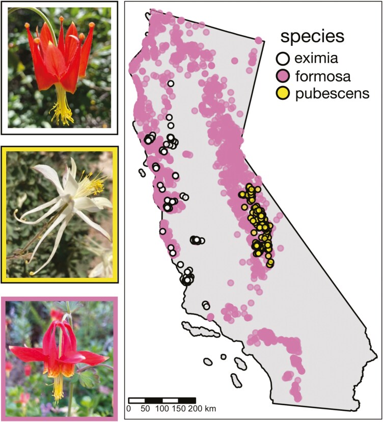 Fig. 1
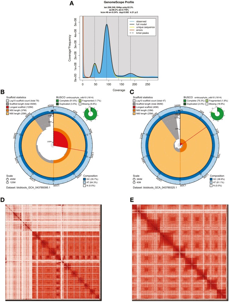 Fig. 2
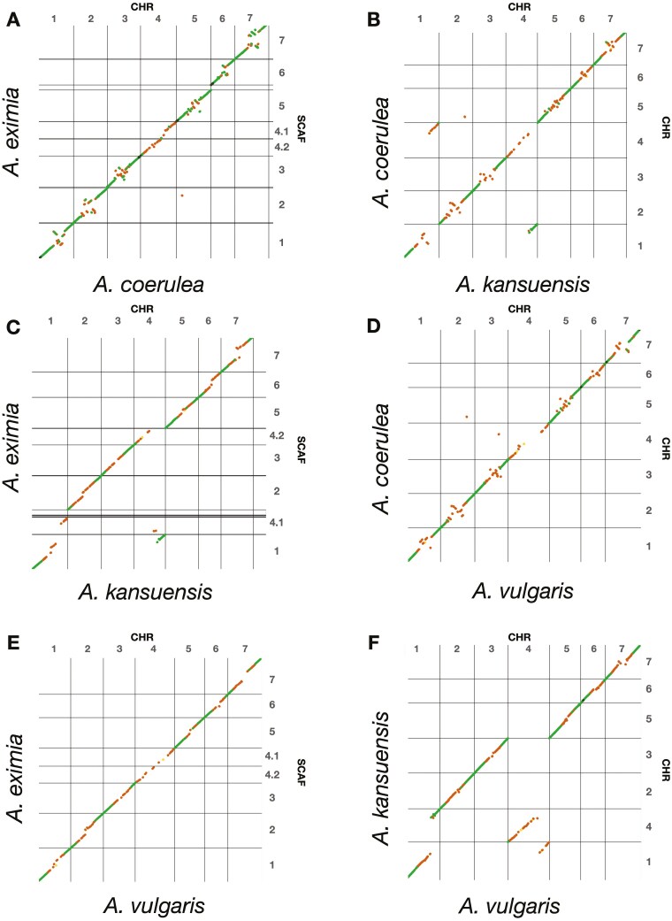 Fig. 3
| Assembly step | Software and any non-default options | Version | References |
|---|---|---|---|
| Initial assembly | |||
| Filtering PacBio HiFi adapters | HiFiAdapterFilt | Commit 64d1c7b |
|
| K-mer counting | Meryl ( | 1 |
|
| Estimation of genome size and heterozygosity | GenomeScope | 2 |
|
| De novo | HiFiasm (Hi-C Mode, –primary, output hic.hap1.p_ctg, hic.hap2.p_ctg) | 0.16.1-r375 |
|
| Scaffolding | |||
| Omni-C data alignment | Arima Genomics Mapping Pipeline | Commit 2e74ea4 |
|
| Arima Genomics Mapping Pipeline (AGMP) | BWA-MEM | 0.7.17-r1188 |
|
| Samtools | 1.11 |
| |
| filter_five_end.pl (AGMP) | Commit 2e74ea4 |
| |
| two_read_bam_combiner.pl (AGMP) | Commit 2e74ea4 |
| |
| Picard | 2.27.5 |
| |
| Omni-C Scaffolding | SALSA (-DNASE, -i 20, -p yes) | 2 |
|
| Omni-C Contact map generation | |||
| Short-read alignment | BWA-MEM (-5SP) | 0.7.17-r1188 |
|
| SAM/BAM processing | Samtools | 1.11 |
|
| SAM/BAM filtering | Pairtools | 0.3.0 |
|
| Pairs indexing | Pairix | 0.3.7 |
|
| Matrix generation | Cooler | 0.8.10 |
|
| Matrix balancing | hicExplorer (hicCorrectmatrix correct --filterThreshold -2 4) | 3.6 |
|
| Contact map visualization | HiGlass | 2.1.11 |
|
| PretextMap | 0.1.4 |
| |
| PretextView | 0.1.5 |
| |
| PretextSnapshot | 0.0.3 |
| |
| Manual curation tools | Rapid curation pipeline (Wellcome Trust Sanger Institute, Genome Reference Informatics Team) | Commit 7acf220c |
|
| Genome quality assessment | |||
| Basic assembly metrics | QUAST (--est-ref-size) | 5.0.2 |
|
| Assembly completeness | BUSCO (-m geno, -l embryophyta) | 5.0.0 |
|
| Merqury | 2020-01-29 |
| |
| Contamination screening | |||
| Local alignment tool | BLAST + (-db nt, -outfmt “6 qseqid staxids bitscore std,” -max_target_seqs 1, -max_hsps 1, -evalue 1e-25) | 2.15 |
|
| General contamination screening | BlobToolKit (HiFi coverage, BUSCO = embryophyta, NCBI Taxa ID = 1291435) | 2.3.3 |
|
| Genome comparison | |||
| Synteny plot | D-Genies (using minimap2, “hide noise”) | D-genies version 1.5.0 (minimap2 version 2) used in dgenies) |
|
| Bio Projects and vouchers | CCGP NCBI BioProject | PRJNA720569 | |||||
|---|---|---|---|---|---|---|---|
| Genera NCBI BioProject | PRJNA766267 | ||||||
| Species NCBI BioProject | PRJNA808326 | ||||||
| NCBI BioSample | SAMN25872407 | ||||||
| Specimen identification | PFEx6 | ||||||
| NCBI Genome accessions | Primary | Alternate | |||||
| Assembly accession | |||||||
| Genome sequences | GCA_023053565.2 | GCA_023053535.2 | |||||
| Genome Sequence | PacBio HiFi reads | Run | 1 PACBIO_SMRT (Sequel II) run: 802,141 spots, 10.8G bases, 6.6Gb | ||||
| Accession | SRX15223256 | ||||||
| Omni-C Illumina reads | Run | 2 ILLUMINA (Illumina NovaSeq 6000) runs: 39.1M spots, 11.8G bases, 4Gb | |||||
| Accession | SRX15223257, SRX15223258 | ||||||
| Genome Assembly Quality Metrics | Assembly identifier (Quality code) | dmAquExim1(6.7.P6.Q61.C95) | |||||
| HiFi Read coverage | 29.52X | ||||||
| Primary | Alternate | ||||||
| Number of contigs | 382 | 281 | |||||
| Contig N50 (bp) | 6,093,045 | 6,553,555 | |||||
| Contig NG50 | 6,093,045 | 6,553,555 | |||||
| Longest Contigs | 20,832,410 | 16,749,726 | |||||
| Number of scaffolds | 265 | 185 | |||||
| Scaffold N50 | 47,382,029 | 48,063,828 | |||||
| Scaffold NG50 | 47,382,029 | 48,063,828 | |||||
| Largest scaffold | 56,061,779 | 55,609,086 | |||||
| Size of final assembly | 363,407,297 | 365,358,954 | |||||
| Phased block NG50 | 6,093,045 | 6,553,555 | |||||
| Gaps per Gbp (# Gaps) | 322(117) | 263(96) | |||||
| Indel QV (Frame shift) | 50.37125354 | 50.50182051 | |||||
| Base pair QV | 61.85 | 62.95 | |||||
| Full assembly = 62.37 | |||||||
| k-mer completeness | 91.43 | 91.51 | |||||
| Full assembly = 98.46 | |||||||
| BUSCO completeness (embryophyta) | C | S | D | F | M | ||
| P | 98.02% | 94.30% | 3.72% | 1.18% | 0.81% | ||
| A | 98.02% | 94.30% | 3.72% | 1.12% | 0.87% | ||
| Total size | # contigs | Contig N50 | # scaffolds | Scaffold N50 | BUSCO completeness | Sequencing technology | |
|---|---|---|---|---|---|---|---|
|
| 363 Mb | 382 | 5.0 Mb | 265 | 47.4 Mb | 98.0% | PacBio, Omni-C |
|
| 292 Mb | 7930 | 110 kb | 1034 | 43.6 Mb | 97.2% | Sanger, short-read Illumina |
|
| 293 Mb | 852 | 2.22 Mb | 679 | 40.9 Mb | 97.9% | Illumina, PacBio, BioNano, Hi-C |
|
| 296 Mb | 567 | 1.2Mb | 134 | 42.7Mb | 98.3% | PacBio, Arima2 |
- —University of California by the State of California
Peer Reviews
No public reviews on file for this paper yet. If you reviewed it on a platform where reviews are public (OpenReview, ICLR, NeurIPS, ICML), you can paste yours below so the community can read it here.
Videos
No videos yet. Explain this paper in a talk, walkthrough, or lecture? Add one.
Taxonomy
TopicsChromosomal and Genetic Variations · Plant Diversity and Evolution · Genetic diversity and population structure
Introduction
Aquilegia (columbines) is a genus of flowering plants of ca. 70 species (Munz 1946), having adapted to a wide variety of habitats and pollinators across the Northern Hemisphere over a short evolutionary timespan estimated at ca. 6 to 7 My (Whittall and Hodges 2007; Bastida et al. 2010; Fior et al. 2013; Zhai et al. 2019). In California, there are 3 predominant species, the widespread A. formosa Fish. ex DC. (Hook 1881), and 2 endemic species, A. eximia Van Houtte ex Planch (Planch 1857) and A. pubescens (Coville 1893). Our goal here is to develop a high-quality reference genome that is suitable for assessing genetic diversity of all 3 species, allowing us to assess both a widespread species and those in extreme habitats.
Aquilegia formosa is found from northern Mexico to Alaska and occurs in 10/13 USDA ecoregions across the Southern California Mountains, Northern California Coast and Interior Coast Ranges, Klamath Range, the Southern, Central, and Northern California Coast, Sierra Nevada, Modoc Plateau, and the Northwest Basin and Range. This species has a very wide elevational distribution in California, from sea level to the tree line in the southern Sierra Nevada (~3,000 m), and encompasses the ranges of A. eximia and A. pubescens (Fig. 1). Thus, A. formosa is a good model for studying widespread California plant species, and the dynamics underlying their genetic variation across the landscape.
Photographs and observations of Aquilegia (columbine) species included in the CCGP study. Observation data are based on iNaturalist and personal collections. Border colors around photos correspond to the color of the dots on the range map.
Aquilegia eximia’s range spans 6 USDA (United States Department of Agriculture) ecoregions along the central coastal mountains. The species is found almost exclusively in seeps crossing serpentine soil. Serpentine soils harbor just 1% of California’s land, but 12.5% of its endemic species, which have adapted to the shallow, nutrient poor, with high Mg/Ca and heavy metal-rich soils (Harrison et al. 2006). This species is likely derived from within A. formosa (Whittall and Hodges 2007) and will be an important model for understanding the genetic connectivity across “islands” of serpentine habitat.
Aquilegia pubescens is also endemic to California and is found primarily above the tree line in 1 just USDA ecoregion, the southern Sierra Nevada mountains (Fig. 1). It is very closely related to A. formosa and A. eximia (Whittall and Hodges 2007) and forms natural hybrid zones with A. formosa where their distributions overlap (Hodges and Arnold 1994; Chase and Raven 1975; Grant 1976). This species is representative of high alpine species, allowing us to study connectivity and drivers of genetic diversity in this habitat threatened by climate change.
While there are 3 current genome assemblies for Aquilegia, each have compromises for an assessment of genetic diversity within and across species in California. The first genome assembly for the genus was from a horticultural derivative of a North American species, A. coerulea “Goldsmith,” henceforth referred to as A. coerulea. This genome was assembled prior to high-throughput long-read sequencing and proximity ligation technologies, using Sanger sequencing of a variety of plasmid insert sizes, mapping of F2 recombinant populations, and short-read Illumina sequences (Filiault et al. 2018). As such, the ordering of scaffolds within low recombination regions and high repeats such as pericentric regions was difficult. In fact, multiple QTL analyses of F2 populations using this genome to identify recombination breakpoints have required manual reordering of genomic blocks in these regions (Filiault et al. 2018; Ballerini et al. 2020; Edwards et al. 2021; Johns et al. 2024). A second genome assembly has been constructed for A. oxysepala var. kansuensis, which is a species from central Asia and substantially more distantly related from the California species. Alignment of resequencing data between species from different continents declines significantly (Filiault et al. 2018) making this genome a less useful reference for population genomic analyses in North American taxa. For example, comparison between the A. coerulea and A. oxysepala var. kansuensis genomes revealed a reciprocal translocation between chromosomes (Xie et al. 2020). The third previously assembled Aquilegia genome is for A. vulgaris, a species native to Europe and also relatively distantly related to North American species (NCBI accession GCA_964291885.1; Filiault et al. 2018). Thus, we chose to assemble a new genome sequence using the California endemic species, A. eximia. We chose to use A. eximia as its populations are usually small and isolated from 1 another, making inbreeding more likely, which would reduce heterozygosity and aid in genome assembly. All of these factors will make the A. eximia genome an important tool for aligning resequencing data for population genomic analyses such as the California Conservation Genomics Project (CCGP), as well as providing a more accurate reference genome for future population genomic and trait mapping studies (Shaffer et al. 2022).
Methods
Biological materials
We collected young leaves and floral tissue from a single individual grown from seed collected at Prefumo Canyon in San Luis Obispo County (34.417153, −119.842861). To collect tissue with reduced starch and secondary metabolites, the plant was placed in the dark for 3 to 4 days and then young expanding tissue was collected, weighed, snap frozen, and stored at −80 °C. We then returned the plant to the greenhouse to recover and produce more young tissue and repeated the collection cycle until we had a total of approximately 12 g of tissue.
PacBio HiFi library preparation
High molecular weight (HMW) genomic DNA (gDNA) was extracted from 75 mg of leaves (PF Ex 6) using the Nanobind Plant Nuclei Big DNA Kit (Pacific BioSciences—PacBio, Menlo Park, CA) and (Workman et al. 2018) protocol with the following modification. We used nuclear isolation buffer supplemented with 350 mM Sorbitol to resuspend ground tissue and during the first wash of the nuclei pellet. The DNA purity was estimated using absorbance ratios (260/280 = 1.84 and 260/230 = 2.07) on the NanoDrop ND-1000 spectrophotometer. The final DNA yield (20 μg) was quantified using the Quantus Fluorometer (QuantiFluor ONE dsDNA Dye assay; Promega, Madison, WI). The size distribution of the HMW DNA was estimated using the Femto Pulse system (Agilent, Santa Clara, CA), and found that 70% of the fragments were 120 kb or more.
The HiFi SMRTbell library was constructed using the SMRTbell Express Template Prep Kit v2.0 (PacBio, Cat. No. 100-938-900) according to the manufacturer’s instructions. HMW gDNA was sheared to a target DNA size distribution between 15 and 18 kb. The sheared gDNA was concentrated using 0.45× of AMPure PB beads (PacBio, Cat. No. 100-265-900) for the removal of single-strand overhangs at 37 °C for 15 min, followed by further enzymatic steps of DNA damage repair at 37 °C for 30 min, end repair and A-tailing at 20 °C for 10 min and 65 °C for 30 min, and ligation of overhang adapter v3 at 20 °C for 60 min. The SMRTbell library was purified and concentrated with 1× AMPure PB beads (PacBio, Cat. No. 100-265-900) for nuclease treatment at 37 °C for 30 min and size selection using the BluePippin/PippinHT system (Sage Science, Beverly, MA; Cat. No. BLF7510/HPE7510) to collect fragments greater than 9 kb. The 15 – 20 kb average HiFi SMRTbell library was sequenced at UC Davis DNA Technologies Core (Davis, CA) using 0.5 8M SMRT cell, Sequel II sequencing chemistry 2.0, and 30-h movies on a PacBio Sequel IIe sequencer.
Omni-C library preparation and sequencing
The Omni-C library was prepared using the Dovetail Omni-C Kit (Dovetail Genomics, Scotts Valley, CA) according to the manufacturer’s protocol with slight modifications. First, specimen tissue (leaves, ID: PF Ex 6) was thoroughly ground with a mortar and pestle while cooled with liquid nitrogen. Nuclear isolation was then performed using published methods (Workman et al. 2018). Subsequently, chromatin was fixed in place in the nucleus and digested under various conditions of DNase I until a suitable fragment length distribution of DNA molecules was obtained. Chromatin ends were repaired and ligated to a biotinylated bridge adapter followed by proximity ligation of adapter-containing ends. After proximity ligation, crosslinks were reversed, and the DNA was purified from proteins. Purified DNA was treated to remove biotin that was not internal to ligated fragments. An NGS library was generated using an NEB Ultra II DNA Library Prep kit (New England Biolabs, Ipswich, MA) with an illumine-compatible y-adaptor. Biotin-containing fragments were then captured using streptavidin beads. The post-capture product was split into 2 replicates prior to PCR enrichment to preserve library complexity with each replicate receiving unique dual indices. The library was sequenced at Vincent J. Coates Genomics Sequencing Lab (Berkeley, CA) on an Illumina NovaSeq 6000 platform to generate approximately 100 million 2 × 150 bp read pairs per gigabase of genome size.
DNA sequencing and genome assembly
Nuclear genome assembly.
We assembled the genome of an A. eximia sample following the CCGP assembly pipeline V5.0, which uses PacBio HiFi reads and Omni-C data to produce high quality and highly contiguous genome assemblies. The pipeline is outlined in Table 1 and lists the tools and non-default parameters used in the assembly process. First, we removed the remnants adapter sequences from the PacBio HiFi dataset using HiFiAdapterFilt (Sim et al. 2022) and generated the initial phased diploid assembly using HiFiasm (Cheng et al. 2021, 2022) on Hi-C mode, with the filtered PacBio HiFi reads and the Omni-C dataset. We aligned the Omni-C data to both assemblies following the Arima Genomics Mapping Pipeline (https://github.com/ArimaGenomics/mapping_pipeline) and then scaffolded both assemblies with SALSA (Ghurye et al. 2017, 2019).
Assemblies were manually curated by iteratively generating and analyzing their corresponding Omni-C contact maps. To generate the contact maps we aligned the Omni-C data with BWA-MEM (Li 2013), identified ligation junctions, and generated Omni-C pairs (Lee et al. 2022) using pairtools (Open2C et al. 2024). We generated a multi-resolution Omni-C matrix with cooler (Abdennur and Mirny 2020) and balanced it with hicExplorer (Ramírez et al. 2018). We used HiGlass (Kerpedjiev et al. 2018) and the PretextSuite (https://github.com/wtsi-hpag/PretextView; https://github.com/wtsi-hpag/PretextMap; https://github.com/wtsi-hpag/PretextSnapshot) to visualize the contact maps where we identified misassemblies and misjoins, and finally modified the assemblies using the Rapid Curation pipeline from the Wellcome Trust Sanger Institute, Genome Reference Informatics Team (https://gitlab.com/wtsi-grit/rapid-curation). Some of the remaining gaps (joins generated during scaffolding and/or curation) were closed using the PacBio HiFi reads and YAGCloser (https://github.com/merlyescalona/yagcloser). Finally, we checked for contamination using the BlobToolKit Framework (Challis et al. 2020).
Genome quality assessment.
We generated k-mer counts from the PacBio HiFi reads using meryl (https://github.com/marbl/meryl). The k-mer counts were then used in GenomeScope2.0 (Ranallo-Benavidez et al. 2020) to estimate genome features including genome size, heterozygosity, and repeat content. For contiguity metrics, we ran QUAST (Gurevich et al. 2013). To evaluate genome quality and functional completeness we used BUSCO (Manni et al. 2021) with the Embryophyta ortholog database (embryophyta_odb10) which contains 1,614 genes. Assessment of base level accuracy (QV) and k-mer completeness was performed using the previously generated meryl database and merqury (Rhie et al. 2020). We further estimated genome assembly accuracy via BUSCO gene set frameshift analysis using the pipeline described in (Korlach et al. 2017). Measurements of the size of the phased blocks is based on the size of the contigs generated by HiFiasm on HiC mode. We follow the quality metric nomenclature established by Rhie et al. (2021), with the genome quality code x·y·P·Q·C, where, x = log_10_[contig NG50]; y = log_10_[scaffold NG50]; P = log_10_ [phased block NG50]; Q = Phred base accuracy QV (quality value); C = % genome represented by the first “n” scaffolds, following a karyotype of 2n = 14, known for the number of chromosomes for this species (Genome on a Tree—GoaT; tax_tree [A. eximia; Challis et al. 2023]). Quality metrics for the notation were calculated on the assembly for the primary haplotype.
Comparison to other Aquilegia spp.
To assess broad synteny and genome structure we generated dot plots with D-Genies (Cabanettes and Klopp 2018) among 3 other publicly available genomes: A. kansuensis (Xie et al. 2020), A. coerulea (Filiault et al. 2018), and A. vulgaris (NCBI accession GCA_964291885.1). We used the 8 largest scaffolds of A. eximia to reduce complexity.
Results
Sequencing data
The Omni-C library generated 39.08 million read pairs and the PacBio SMRTBell library generated 802.07 thousand HiFi reads. The PacBio HiFi reads yielded ~29× genome coverage and had an N50 read length of 14,254 bp; a minimum read length of 123 bp; a mean read length of 13,508 bp; and a maximum read length of 46,837 bp (see Supplementary Fig. S1 for read length distribution). Based on the PacBio HiFi data, Genomescope 2.0 estimated a genome size of 367 Mb, a 0.559% heterozygosity rate and a 0.131% sequencing error rate. The k-mer spectrum shows a bimodal distribution with a major peak at ~29-fold coverage and a minor peak at ~15-fold coverage (Fig. 2a).
Overview of genome assembly metrics for Aquilegia eximia. a) K-mer spectrum output from PacBio HiFi data without adapters, generated using GenomeScope2.0. K-mers at lower coverage and lower frequency correspond to differences between haplotypes, whereas the higher coverage and higher frequency k-mers correspond to the similarities between haplotypes. B and c) Snail plots for the primary (b) and alternate (c) genome assembly showing a graphical representation of the quality metrics in Table 2 for the primary assembly. The circle represents the full size of the assembly. From the inside-out, the central plot displays length-related metrics. The red line represents the longest scaffold; other scaffolds are ordered by size moving clockwise around the plot and drawn in gray starting from the outside of the central plot. Dark and light orange arcs mark the scaffold N50 and N90 values. The central light gray spiral shows the cumulative scaffold count with a white line at each order of magnitude. White regions in this area reflect the proportion of Ns in the assembly The dark versus light blue area around it shows mean, maximum, and minimum GC versus AT content at 0.1% intervals (Challis et al. 2020). d and e) Hi-C Contact maps for the primary (d) and alternate (e) genome assembly generated with PretextSnapshot. Hi-C contact maps translate the proximity of genomic regions in 3-D space to contiguous linear organization. Each cell in the contact map corresponds to sequencing data supporting the linkage (or join) between 2 of such regions. Scaffolds numbers are indicated and are separated by black lines. Higher density corresponds to higher levels of fragmentation.
Nuclear genome assembly
The final genome assembly (dmAquExim1) consists of 2 phased haplotypes, however, the assemblies have been randomly tagged as primary and alternate. Both assemblies are similar in size, with a difference of ~2 Mb between haplotypes. The final assemblies are also similar in size but not equal to the estimated genome assembly size from GenomeScope2.0, as it has been observed in other taxa (see Pflug et al. 2020, e.g.).
The primary haplotype (dmAquExim1.1.p) consists of 265 scaffolds spanning 363.4 Mb with a contig N50 of 6.09 Mb, a scaffold N50 of 47.38 Mb, the largest contig size of 20.83 Mb, and the largest scaffold size of 56.05 Mb. The alternate haplotype (dmAquExim1.1.a) consists of 185 scaffolds spanning 365.35 Mb with a contig N50 of 6.55 Mb, a scaffold N50 of 48.06 Mb, the largest contig size of 16.74 Mb, and the largest scaffold size of 55.6 Mb.
The primary haplotype has a BUSCO completeness score for the Embryophyta gene set of 97.8%, a base pair quality value (QV) of 61.85, a kmer completeness of 91.43%, and a frameshift indel QV of 50.83. The alternate haplotype has a BUSCO completeness score for the same gene set of 97.9%, a base pair QV of 62.95, a kmer completeness of 91.51%, and a frameshift indel QV of 50.32.
During manual curation we made a total of 167 joins (96 on the primary haplotype and 71 on the alternate haplotype) and 53 breaks (29 on the primary haplotype and 24 on the alternate haplotype) based on the signal from the Omni-C contact maps. We were able to close a total of 39 gaps, 20 on the primary haplotype and 19 on the alternate. No other contigs were modified or removed.
The Omni-C contact maps show highly contiguous assembly, suggesting that the A. eximia genome is organized in 8 major scaffolds based on the number of major bins along the diagonal axis of the plot, corresponding to 95.6% of the genome size (Fig. 2c and d). Assembly statistics are reported in Table 2 and represented graphically in Fig. 2c. We have deposited the genome assembly on NCBI GenBank (see Table 2 s details).
Comparison with other Aquilegia genome assemblies
BUSCO analysis revealed high completeness of 97.8%, similar to the scores for the assemblies of A. coerulea (97.2%), A. kansuensis (97.9%), and A. vulgaris (98.3%). The estimated genome size, 367 Mb, is significantly larger than those found for the other 3 Aquilegia genome assemblies (Table 3).
Dot plots between A. coerulea and A. kansuensis reflected the results of (Xie et al. 2020), where the 7 chromosomes aligned to each other in large contiguous blocks of synteny except in presumably pericentromeric regions and an apparent reciprocal translocation between chromosomes 1 and 4 (Fig. 3a). In addition, in the pericentromeric regions, there are many smaller blocks of synteny but with scrambled relative orders and orientations. Comparing A. eximia to A. coerulea, A. kansuensis, and A. vulgaris revealed that the A. eximia assembly is near-chromosome level, where the largest 8 scaffolds of A. eximia were syntenic with the 7 chromosomes of the other species (Fig 3b and c). The alignment between A. eximia and A. vulgaris was relatively contiguous with no major rearrangements. Because the genome assembled into 8 large scaffolds rather than 7 as expected from the canonical chromosome number for the genus, we especially scrutinized the contact maps surrounding scaffolds 4.1 and 4.2, which align with chromosome 4 of A. coerulea and A. vulgaris (Fig. 2d and e and Supplementary Fig. S2). We found no convincing evidence from these data to merge scaffolds 4.1 and 4.2 into a single scaffold.
Dot plot alignments comparing Aquilegia genome assemblies: 7 chromosomes (labeled) for A. coerulea, A. kansuensis, and A. vulgaris, and the 8 largest scaffolds in A. eximia which are homologous with the 7 chromosomes in the other 3 species (labeled). We modified the chromosome numbers in A. vulgaris to match their homologs in A. coerulea and A. kansuensis.
Notably, A. eximia, A. coerula, and A. vulgaris all share overall similar chromosome structures without any large translocations (Fig. 3a, d, and e). Specifically, all of scaffold 1 of A. eximia aligns with chromosome 1 of A. coerulea and A. vulgaris, and scaffolds 4.1 (JALIGU020000007.1) and 4.2 (JALIGU020000008.1) of A. eximia align to chromosome 4 of A. coerulea and A. vulgaris. However, when A. eximia is compared with A. kansuensis, the same reciprocal translocation between chromosomes 1 and 4 of A. coerulea/A. kansusensis was found (Fig. 3c). Furthermore, the A. eximia chromosomes show much higher contiguity in paracentric regions with A. kansuensis and A. vulgaris than with the more closely related A. coerulea. These 3 species, when compared to A. coerulea, each show scrambling of the relative orders and orientations of smaller synteny blocks in pericentromeric regions (Fig. 3a, b, and d) but when compared to each other, they show high contiguity (Fig. 3c, e, and f). This suggests that the ordering and orientation of scaffolds in the pericentromeric regions of the A. coerulea genome may be somewhat misplaced.
Discussion
Here we present the first de novo reference genome for the California endemic, serpentine-adapted columbine, A. eximia. Three other genome assemblies are available for Aquilegia species and the A. eximia genome assembly has the highest contig N50 at 5.0 Mb (compared to A. kansuensis at 2.2 Mb, A. vulgaris at 1.2 Mb, and A. coerulea at 110 kb) as well as the highest scaffold N50 at 47.4 Mb (compared to A. coerulea at 43.6 Mb, A. vulgaris at 42.7 Mb, and A. kansuensis at 40.9 Mb; Filiault et al. 2018; Xie et al. 2020). The A. eximia genome assembly also has a BUSCO completeness score that is very high (98.0%), similar to other Aquilegia genome assemblies (Table 3). Lastly, the A. eximia genome is significantly larger, spanning 363 Mb, compared to genome sizes of 292 to 296 Mb for A. coerulea, A. kansuensis, and A. vulgaris. This larger genome size is reflected across each of the 7 chromosomes (counting A. eximia scaffolds 4.1 and 4.2 together when comparing to chromosome 4 of the other species).
We further compared the structure of Aquilegia genome assemblies using dot plots and found, overall, very similar structures. The most striking difference is that the A. eximia assembles into 8 large scaffolds (26.3 to 56.0 Mb) while the 3 other Aquilegia genomes each assemble into 7 large scaffolds. The canonical karyotype of Aquilegia species is n = 7 (Gregory 1941; Taylor 1967) although there are at least 7 species with reports of karyotypes of both n = 7 and n = 8 (Dawe and Murray 1981; Subramanian 1985; Chung et al. 2013). The A. eximia scaffolds 4.1 and 4.2 align with chromosome 4 of A. coerulea and A. vulgaris (Fig. 3a and e) suggesting that either chromosome 4 has split into 2 chromosomes in A. eximia or that our data are insufficient to merge these 2 scaffolds together (Supplementary Fig. S2). Future studies of karyotypes, recombination maps and FISH analysis would be useful in resolving these possibilities. In addition, it is interesting that chromosome 4 is involved with this difference in scaffold numbers because chromosome 4 has many enigmatic characteristics compared to the other chromosomes such as a higher rate of polymorphism, lower gene density, lower gene expression, as well as harboring the 5S and 35S rDNA repeats (Filiault et al. 2018). As previously reported, A. kansuensis differs in chromosome structure from A. coerulea due to a reciprocal translocation between chromosomes 1 and 4 (Xie et al. 2020) and our data shows that A. eximia shares the structure of A. coerulea as does A. vulgaris (Fig. 3a and e). Lastly, overall, the A. eximia genome shows much more contiguous alignments, especially in paracentric regions, with A. kansuensis and A. vulgaris than with A. coerulea (Fig. 3). This is likely due to mis-assembly of the A. coerulea genome, which is the only assembly that lacked Hi-C data.
Given the high contiguity and completeness of the A. eximia genome, it will be an excellent reference genome for population genetic studies and genetic mapping studies, especially for closely related North American taxa. Furthermore, it has an especially close phylogenetic relationship with A. formosa and A. pubescens. Thus, it is a strong asset for the goals of the CCGP and for studying plant adaptation to some of California’s most important contributors to biodiversity, such as serpentine soil, high alpine, and riparian corridors.
Supplementary material
Supplementary material is available at Journal of Heredity online.
esaf035_suppl_Supplementary_Figures_S1-S2
The reference list from the paper itself. Each links out to its DOI / PubMed record.
- 1Abdennur N, Fudenberg G, Flyamer IM, Galitsyna AA, Goloborodko A, Imakaev M, Venev SV; Open 2C. Pairtools: from sequencing data to chromosome contacts. P Lo S Comput Biol. 2024:20:e 1012164.38809952 10.1371/journal.pcbi.1012164 PMC 11164360 · doi ↗ · pubmed ↗
- 2Abdennur N, Mirny LA. Cooler: scalable storage for Hi-C data and other genomically labeled arrays. Bioinformatics. 2020:36:311–316.31290943 10.1093/bioinformatics/btz 540PMC 8205516 · doi ↗ · pubmed ↗
- 3Ballerini ES, Min Y, Edwards MB, Kramer EM, Hodges SA. POPOVICH, encoding a C 2H 2 zinc-finger transcription factor, plays a central role in the development of a key innovation, floral nectar spurs, in Aquilegia. Proc Natl Acad Sci U S A. 2020:117:22552–22560.32848061 10.1073/pnas.2006912117 PMC 7486772 · doi ↗ · pubmed ↗
- 4Bastida JM, Alcántara JM, Rey PJ, Vargas P, Herrera CM. Extended phylogeny of Aquilegia: the biogeographical and ecological patterns of two simultaneous but contrasting radiations. Plant Syst Evol. 2010:284:171–185.
- 5Cabanettes F, Klopp C. D-GENIES: dot plot large genomes in an interactive, efficient and simple way. Peer J. 2018:6:e 4958.29888139 10.7717/peerj.4958 PMC 5991294 · doi ↗ · pubmed ↗
- 6Camacho C, Coulouris G, Avagyan V, Ma N, Papadopoulos J, Bealer K, Madden TL. BLAST+: architecture and applications. BMC Bioinf. 2009:10:421.10.1186/1471-2105-10-421PMC 280385720003500 · doi ↗ · pubmed ↗
- 7Challis R, Kumar S, Sotero-Caio C, Brown M, Blaxter M. Genomes on a Tree (Goa T): a versatile, scalable search engine for genomic and sequencing project metadata across the eukaryotic tree of life. Wellcome Open Res. 2023:8:24.36864925 10.12688/wellcomeopenres.18658.1PMC 9971660 · doi ↗ · pubmed ↗
- 8Challis R, Richards E, Rajan J, Cochrane G, Blaxter M. Blob Tool Kit - interactive quality assessment of genome assemblies. G 3 (Bethesda). 2020:10:1361–1374.32071071 10.1534/g 3.119.400908 PMC 7144090 · doi ↗ · pubmed ↗