The genome sequence of the Tenthredid wasp, Eutomostethus luteiventris (Klug, 1816) (Hymenoptera: Tenthredinidae)
Andrew Halstead, Keith Fowler, Annabel Whibley, Arun Arumugaperumal, Benoit Nabholz, Qing-Song Zhou

TL;DR
This paper provides a detailed genome sequence of the Tenthredid wasp Eutomostethus luteiventris as part of a broader project to map species genomes in Britain and Ireland.
Contribution
The novel contribution is the first haploid genome assembly of Eutomostethus luteiventris, including a detailed mitochondrial genome.
Findings
The genome assembly is 272.06 megabases long with 99.22% scaffolded into 6 chromosomal pseudomolecules.
The mitochondrial genome is 30.01 kilobases long and fully assembled.
The work is part of the Darwin Tree of Life project focusing on eukaryotic species in Britain and Ireland.
Abstract
We present a haploid genome assembly from an individual Eutomostethus luteiventris (Tenthredid wasp; Arthropoda; Insecta; Hymenoptera; Tenthredinidae). The genome sequence has a total length of 272.06 megabases. Most of the assembly (99.22%) is scaffolded into 6 chromosomal pseudomolecules. The mitochondrial genome has also been assembled, with a length of 30.01 kilobases. This assembly was generated as part of the Darwin Tree of Life project, which produces reference genomes for eukaryotic species found in Britain and Ireland.
Genes, proteins, chemicals, diseases, species, mutations and cell lines named across the full text — each resolved to its canonical identifier and authoritative record.
Click any figure to enlarge with its caption.
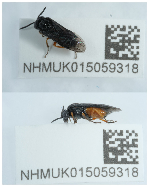 Figure 1
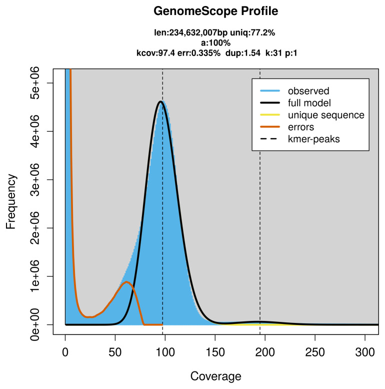 Figure 2
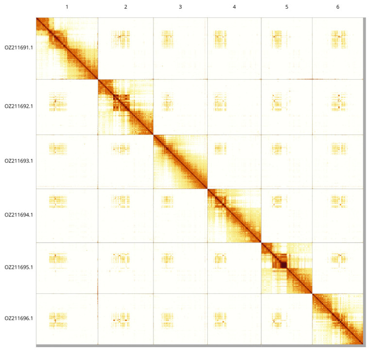 Figure 3
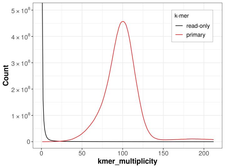 Figure 4
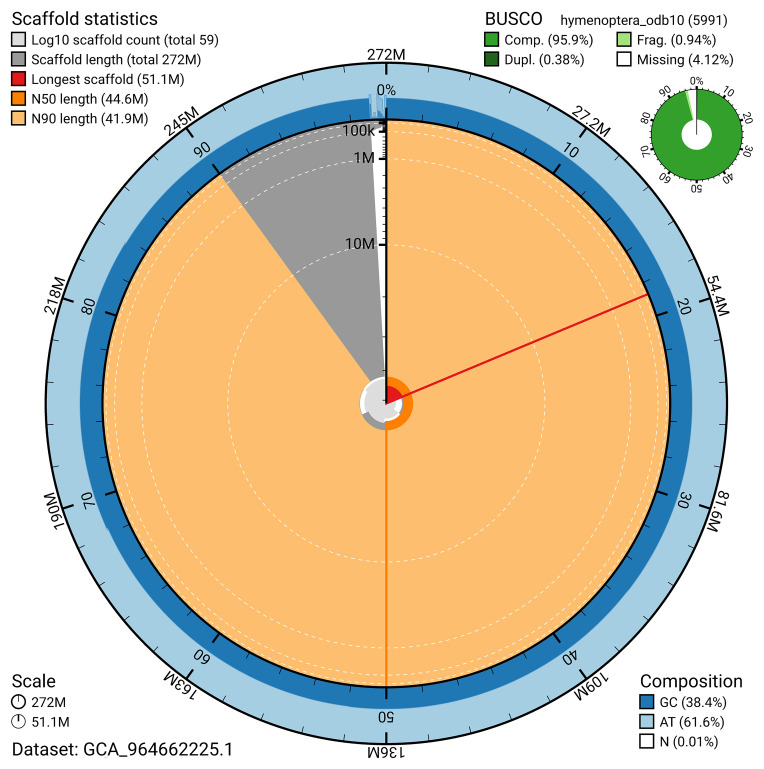 Figure 5
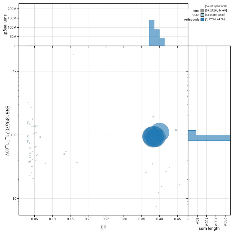 Figure 6
| Platform | PacBio HiFi | Hi-C |
|---|---|---|
|
| iyEutLute1 | iyEutLute1 |
|
| NHMUK015059318 | NHMUK015059318 |
|
| SAMEA112964468 | SAMEA112964468 |
|
| SAMEA112975668 | SAMEA112975668 |
|
| whole organism | whole organism |
|
| Sequel IIe | Illumina NovaSeq 6000 |
|
| ERR13957071 | ERR13947545 |
|
| 2.32 million | 724.51 million |
|
| 25.44 Gb | 109.40 Gb |
|
| iyEutLute1.1 |
|
| GCA_964662225.1 |
|
| chromosome |
|
| 272.06 |
|
| 6 |
|
| 236 |
|
| 4.5 Mb |
|
| 58 |
|
| 44.62 Mb |
|
| Mitochondrion: 30.01 kb |
| INSDC
| Molecule | Length
| GC% |
|---|---|---|---|
| OZ211691.1 | 1 | 51.14 | 38 |
| OZ211692.1 | 2 | 45.64 | 39 |
| OZ211693.1 | 3 | 44.62 | 38.50 |
| OZ211694.1 | 4 | 44.43 | 38 |
| OZ211695.1 | 5 | 42.07 | 40 |
| OZ211696.1 | 6 | 42.05 | 38.50 |
| Measure | Value | Benchmark |
|---|---|---|
| EBP summary (primary) | 6.C.Q65 | 6.C.Q40 |
| Contig N50 length | 4.50 Mb | ≥ 1 Mb |
| Scaffold N50 length | 44.62 Mb | = chromosome N50 |
| Consensus quality (QV) | Primary: 65.2 | ≥ 40 |
|
| Primary: 99.41% | ≥ 95% |
| BUSCO | C:95.9% [S:95.5%;
| S > 90%; D < 5% |
| Percentage of
| 99.22% | ≥ 90% |
- —Wellcome Trust
Peer Reviews
No public reviews on file for this paper yet. If you reviewed it on a platform where reviews are public (OpenReview, ICLR, NeurIPS, ICML), you can paste yours below so the community can read it here.
Videos
No videos yet. Explain this paper in a talk, walkthrough, or lecture? Add one.
Taxonomy
TopicsPlant and animal studies · Insect and Arachnid Ecology and Behavior · Fossil Insects in Amber
Species taxonomy
Eukaryota; Opisthokonta; Metazoa; Eumetazoa; Bilateria; Protostomia; Ecdysozoa; Panarthropoda; Arthropoda; Mandibulata; Pancrustacea; Hexapoda; Insecta; Dicondylia; Pterygota; Neoptera; Endopterygota; Hymenoptera; Tenthredinoidea; Tenthredinidae; Blennocampinae; Eutomostethus; Eutomostethus luteiventris (Klug, 1816) (NCBI:txid1385253)
Background
Eutomostethus luteiventris is a species in which only females have been recorded in Britain and Ireland, and reproduction is believed to be parthenogenetic. It is 5–7mm long with a black head and thorax. The abdomen is mostly orange-yellow with black markings down the centre of the dorsal surface. It occurs in damp places where the larvae feed inside the foliage of rushes, Juncus spp., with the final instar feeding externally ( Benson, 1952).
Eutomostethus luteiventris a common species throughout Britain and also occurs throughout most of Europe ( GBIF Secretariat, 2024). It is an introduced species in North America. In the UK, there is a single generation with adults occurring in late April to June.
The genome of the sawfly, Eutomostethus luteiventris, was sequenced as part of the Darwin Tree of Life Project, a collaborative effort to sequence all named eukaryotic species in the Atlantic Archipelago of Britain and Ireland ( Blaxter et al., 2022). The assembly was produced using the Tree of Life pipeline from a specimen collected in Thompson Common, Norfolk, United Kingdom ( Figure 1).
Photograph of the Eutomostethus luteiventris (iyEutLute1) specimen used for genome sequencing.
Methods
Sample acquisition and DNA barcoding
The specimen used for genome sequencing was an adult Eutomostethus luteiventris (specimen ID NHMUK015059318, ToLID iyEutLute1; Figure 1), collected from Thompson Common, Norfolk, United Kingdom (latitude 52.53, longitude 0.85) on 2022-07-06. The specimen was collected by Keith Fowler and identified by Andrew Halstead. Sample metadata were collected in line with the Darwin Tree of Life project standards described by Lawniczak et al. (2022).
The initial identification was verified by an additional DNA barcoding process according to the framework developed by Twyford et al. (2024). A small sample was dissected from the specimen and stored in ethanol, while the remaining parts were shipped on dry ice to the Wellcome Sanger Institute (WSI) (see the protocol). The tissue was lysed, the COI marker region was amplified by PCR, and amplicons were sequenced and compared to the BOLD database, confirming the species identification ( Crowley et al., 2023). Following whole genome sequence generation, the relevant DNA barcode region was also used alongside the initial barcoding data for sample tracking at the WSI ( Twyford et al., 2024). The standard operating procedures for Darwin Tree of Life barcoding are available on protocols.io.
Nucleic acid extraction
Protocols for high molecular weight (HMW) DNA extraction developed at the Wellcome Sanger Institute (WSI) Tree of Life Core Laboratory are available on protocols.io ( Howard et al., 2025). The iyEutLute1 sample was weighed and triaged to determine the appropriate extraction protocol. Tissue from the whole organism was homogenised by powermashing using a PowerMasher II tissue disruptor.
HMW DNA was extracted in the WSI Scientific Operations core using the Automated MagAttract v2 protocol. DNA was sheared into an average fragment size of 12–20 kb following the Megaruptor®3 for LI PacBio protocol. Sheared DNA was purified by manual SPRI (solid-phase reversible immobilisation). The concentration of the sheared and purified DNA was assessed using a Nanodrop spectrophotometer and Qubit Fluorometer using the Qubit dsDNA High Sensitivity Assay kit. Fragment size distribution was evaluated by running the sample on the FemtoPulse system. For this sample, the final post-shearing DNA had a Qubit concentration of 14.78 ng/μL and a yield of 665.10 ng, with a fragment size of 12.7 kb. The 260/280 spectrophotometric ratio was 2.07, and the 260/230 ratio was 3.46.
PacBio HiFi library preparation and sequencing
Library preparation and sequencing were performed at the WSI Scientific Operations core. Libraries were prepared using the SMRTbell Prep Kit 3.0 (Pacific Biosciences, California, USA), following the manufacturer’s instructions. The kit includes reagents for end repair/A-tailing, adapter ligation, post-ligation SMRTbell bead clean-up, and nuclease treatment. Size selection and clean-up were performed using diluted AMPure PB beads (Pacific Biosciences). DNA concentration was quantified using a Qubit Fluorometer v4.0 (ThermoFisher Scientific) and the Qubit 1X dsDNA HS assay kit. Final library fragment size was assessed with the Agilent Femto Pulse Automated Pulsed Field CE Instrument (Agilent Technologies) using the gDNA 55 kb BAC analysis kit.
The sample was sequenced using the Sequel IIe system (Pacific Biosciences, California, USA). The concentration of the library loaded onto the Sequel IIe was in the range 40–135 pM. The SMRT link software, a PacBio web-based end-to-end workflow manager, was used to set-up and monitor the run, and to perform primary and secondary analysis of the data upon completion.
Hi-C
** Sample preparation and crosslinking **
The Hi-C sample was prepared from 20–50 mg of frozen whole organism tissue of the iyEutLute1 sample using the Arima-HiC v2 kit (Arima Genomics). Following the manufacturer’s instructions, tissue was fixed and DNA crosslinked using TC buffer to a final formaldehyde concentration of 2%. The tissue was homogenised using the Diagnocine Power Masher-II. Crosslinked DNA was digested with a restriction enzyme master mix, biotinylated, and ligated. Clean-up was performed with SPRISelect beads before library preparation. DNA concentration was measured with the Qubit Fluorometer (Thermo Fisher Scientific) and Qubit HS Assay Kit. The biotinylation percentage was estimated using the Arima-HiC v2 QC beads.
** Hi-C library preparation and sequencing **
Biotinylated DNA constructs were fragmented using a Covaris E220 sonicator and size selected to 400–600 bp using SPRISelect beads. DNA was enriched with Arima-HiC v2 kit Enrichment beads. End repair, A-tailing, and adapter ligation were carried out with the NEBNext Ultra II DNA Library Prep Kit (New England Biolabs), following a modified protocol where library preparation occurs while DNA remains bound to the Enrichment beads. Library amplification was performed using KAPA HiFi HotStart mix and a custom Unique Dual Index (UDI) barcode set (Integrated DNA Technologies). Depending on sample concentration and biotinylation percentage determined at the crosslinking stage, libraries were amplified with 10–16 PCR cycles. Post-PCR clean-up was performed with SPRISelect beads. Libraries were quantified using the AccuClear Ultra High Sensitivity dsDNA Standards Assay Kit (Biotium) and a FLUOstar Omega plate reader (BMG Labtech).
Prior to sequencing, libraries were normalised to 10 ng/μL. Normalised libraries were quantified again and equimolar and/or weighted 2.8 nM pools. Pool concentrations were checked using the Agilent 4200 TapeStation (Agilent) with High Sensitivity D500 reagents before sequencing. Sequencing was performed using paired-end 150 bp reads on the Illumina NovaSeq 6000.
Genome assembly
Prior to assembly of the PacBio HiFi reads, a database of k-mer counts ( k = 31) was generated from the filtered reads using FastK. GenomeScope2 ( Ranallo-Benavidez et al., 2020) was used to analyse the k-mer frequency distributions, providing estimates of genome size, heterozygosity, and repeat content.
The HiFi reads were assembled using Hifiasm ( Cheng et al., 2021) with the --primary option. Haplotypic duplications were identified and removed using purge_dups ( Guan et al., 2020). The Hi-C reads ( Rao et al., 2014) were mapped to the primary contigs using bwa-mem2 ( Vasimuddin et al., 2019), and the contigs were scaffolded in YaHS ( Zhou et al., 2023) with the --break option for handling potential misassemblies. The scaffolded assemblies were evaluated using Gfastats ( Formenti et al., 2022), BUSCO ( Manni et al., 2021) and MERQURY.FK ( Rhie et al., 2020).
The mitochondrial genome was assembled using MitoHiFi ( Uliano-Silva et al., 2023), which runs MitoFinder ( Allio et al., 2020) and uses these annotations to select the final mitochondrial contig and to ensure the general quality of the sequence.
Assembly curation
The assembly was decontaminated using the Assembly Screen for Cobionts and Contaminants ( ASCC) pipeline. TreeVal was used to generate the flat files and maps for use in curation. Manual curation was conducted primarily in PretextView and HiGlass ( Kerpedjiev et al., 2018). Scaffolds were visually inspected and corrected as described by Howe et al. (2021). Manual corrections included 7 breaks and 82 joins. The curation process is documented at https://gitlab.com/wtsi-grit/rapid-curation. PretextSnapshot was used to generate a Hi-C contact map of the final assembly.
Assembly quality assessment
The Merqury.FK tool ( Rhie et al., 2020) was run in a Singularity container ( Kurtzer et al., 2017) to evaluate k-mer completeness and assembly quality for the primary and alternate haplotypes using the k-mer databases ( k = 31) computed prior to genome assembly. The analysis outputs included assembly QV scores and completeness statistics.
The genome was analysed using the BlobToolKit pipeline, a Nextflow implementation of the earlier Snakemake version ( Challis et al., 2020). The pipeline aligns PacBio reads using minimap2 ( Li, 2018) and SAMtools ( Danecek et al., 2021) to generate coverage tracks. It runs BUSCO ( Manni et al., 2021) using lineages identified from the NCBI Taxonomy ( Schoch et al., 2020). For the three domain-level lineages, BUSCO genes are aligned to the UniProt Reference Proteomes database ( Bateman et al., 2023) using DIAMOND blastp ( Buchfink et al., 2021). The genome is divided into chunks based on the density of BUSCO genes from the closest taxonomic lineage, and each chunk is aligned to the UniProt Reference Proteomes database with DIAMOND blastx. Sequences without hits are chunked using seqtk and aligned to the NT database with blastn ( Altschul et al., 1990). The BlobToolKit suite consolidates all outputs into a blobdir for visualisation. The BlobToolKit pipeline was developed using nf-core tooling ( Ewels et al., 2020) and MultiQC ( Ewels et al., 2016), with containerisation through Docker ( Merkel, 2014) and Singularity ( Kurtzer et al., 2017).
Genome sequence report
Sequence data
PacBio sequencing of the Eutomostethus luteiventris specimen generated 25.44 Gb (gigabases) from 2.32 million reads, which were used to assemble the genome. GenomeScope2.0 analysis estimated the haploid genome size at 234.63 Mb, with repeat content of 23.03% ( Figure 2). These estimates guided expectations for the assembly. Based on the estimated genome size, the sequencing data provided approximately 195× coverage. Hi-C sequencing produced 109.40 Gb from 724.51 million reads, which were used to scaffold the assembly. Table 1 summarises the specimen and sequencing details.
Frequency distribution of k-mers generated using GenomeScope2.The plot shows observed and modelled k-mer spectra, providing estimates of genome size, heterozygosity, and repeat content based on unassembled sequencing reads.
Table 1.: Specimen and sequencing data for BioProject PRJEB82369.
<table><thead><tr><th align="left" colspan="1" rowspan="1">Platform</th><th align="left" colspan="1" rowspan="1">PacBio HiFi</th><th align="left" colspan="1" rowspan="1">Hi-C</th></tr></thead><tbody><tr><td align="left" colspan="1" rowspan="1"> <bold>ToLID</bold> </td><td align="left" colspan="1" rowspan="1">iyEutLute1</td><td align="left" colspan="1" rowspan="1">iyEutLute1</td></tr><tr><td align="left" colspan="1" rowspan="1"> <bold>Specimen ID</bold> </td><td align="left" colspan="1" rowspan="1">NHMUK015059318</td><td align="left" colspan="1" rowspan="1">NHMUK015059318</td></tr><tr><td align="left" colspan="1" rowspan="1"> <bold>BioSample (source</bold> <break/> <bold>individual)</bold> </td><td align="left" colspan="1" rowspan="1">SAMEA112964468</td><td align="left" colspan="1" rowspan="1">SAMEA112964468</td></tr><tr><td align="left" colspan="1" rowspan="1"> <bold>BioSample (tissue)</bold> </td><td align="left" colspan="1" rowspan="1">SAMEA112975668</td><td align="left" colspan="1" rowspan="1">SAMEA112975668</td></tr><tr><td align="left" colspan="1" rowspan="1"> <bold>Tissue</bold> </td><td align="left" colspan="1" rowspan="1">whole organism</td><td align="left" colspan="1" rowspan="1">whole organism</td></tr><tr><td align="left" colspan="1" rowspan="1"> <bold>Instrument</bold> </td><td align="left" colspan="1" rowspan="1">Sequel IIe</td><td align="left" colspan="1" rowspan="1">Illumina NovaSeq 6000</td></tr><tr><td align="left" colspan="1" rowspan="1"> <bold>Run accessions</bold> </td><td align="left" colspan="1" rowspan="1">ERR13957071</td><td align="left" colspan="1" rowspan="1">ERR13947545</td></tr><tr><td align="left" colspan="1" rowspan="1"> <bold>Read count total</bold> </td><td align="left" colspan="1" rowspan="1">2.32 million</td><td align="left" colspan="1" rowspan="1">724.51 million</td></tr><tr><td align="left" colspan="1" rowspan="1"> <bold>Base count total</bold> </td><td align="left" colspan="1" rowspan="1">25.44 Gb</td><td align="left" colspan="1" rowspan="1">109.40 Gb</td></tr></tbody></table>Assembly statistics
A single haplotype was assembled, with no evidence of heterozygosity. The final assembly has a total length of 272.06 Mb in 58 scaffolds, with 178 gaps, and a scaffold N50 of 44.62 Mb ( Table 2).
Table 2.: Genome assembly statistics.
<table><tbody><tr><td align="left" colspan="1" rowspan="1"> <bold>Assembly name</bold> </td><td align="left" colspan="1" rowspan="1">iyEutLute1.1</td></tr><tr><td align="left" colspan="1" rowspan="1"> <bold>Assembly accession</bold> </td><td align="left" colspan="1" rowspan="1">GCA_964662225.1</td></tr><tr><td align="left" colspan="1" rowspan="1"> <bold>Assembly level</bold> </td><td align="left" colspan="1" rowspan="1">chromosome</td></tr><tr><td align="left" colspan="1" rowspan="1"> <bold>Span (Mb)</bold> </td><td align="left" colspan="1" rowspan="1">272.06</td></tr><tr><td align="left" colspan="1" rowspan="1"> <bold>Number of </bold> <break/> <bold>chromosomes</bold> </td><td align="left" colspan="1" rowspan="1">6</td></tr><tr><td align="left" colspan="1" rowspan="1"> <bold>Number of contigs</bold> </td><td align="left" colspan="1" rowspan="1">236</td></tr><tr><td align="left" colspan="1" rowspan="1"> <bold>Contig N50</bold> </td><td align="left" colspan="1" rowspan="1">4.5 Mb</td></tr><tr><td align="left" colspan="1" rowspan="1"> <bold>Number of scaffolds</bold> </td><td align="left" colspan="1" rowspan="1">58</td></tr><tr><td align="left" colspan="1" rowspan="1"> <bold>Scaffold N50</bold> </td><td align="left" colspan="1" rowspan="1">44.62 Mb</td></tr><tr><td align="left" colspan="1" rowspan="1"> <bold>Organelles</bold> </td><td align="left" colspan="1" rowspan="1">Mitochondrion: 30.01 kb</td></tr></tbody></table>Most of the assembly sequence (99.22%) was assigned to 6 chromosomal-level scaffolds. These chromosome-level scaffolds, confirmed by Hi-C data, are named according to size ( Figure 3; Table 3). The order and orientation of scaffolds between ~16.66-20.70Mb on Chromosome 5 is unsure.
Hi-C contact map of the Eutomostethus luteiventris genome assembly.Assembled chromosomes are shown in order of size and labelled along the axes, with a megabase scale shown below. The plot was generated using PretextSnapshot.
Table 3.: Chromosomal pseudomolecules in the primary genome assembly of Eutomostethus luteiventris iyEutLute1.
<table><thead><tr><th align="center" colspan="1" rowspan="1">INSDC <break/>accession</th><th align="center" colspan="1" rowspan="1">Molecule</th><th align="center" colspan="1" rowspan="1">Length <break/>(Mb)</th><th align="center" colspan="1" rowspan="1">GC%</th></tr></thead><tbody><tr><td align="center" colspan="1" rowspan="1">OZ211691.1</td><td align="center" colspan="1" rowspan="1">1</td><td align="center" colspan="1" rowspan="1">51.14</td><td align="center" colspan="1" rowspan="1">38</td></tr><tr><td align="center" colspan="1" rowspan="1">OZ211692.1</td><td align="center" colspan="1" rowspan="1">2</td><td align="center" colspan="1" rowspan="1">45.64</td><td align="center" colspan="1" rowspan="1">39</td></tr><tr><td align="center" colspan="1" rowspan="1">OZ211693.1</td><td align="center" colspan="1" rowspan="1">3</td><td align="center" colspan="1" rowspan="1">44.62</td><td align="center" colspan="1" rowspan="1">38.50</td></tr><tr><td align="center" colspan="1" rowspan="1">OZ211694.1</td><td align="center" colspan="1" rowspan="1">4</td><td align="center" colspan="1" rowspan="1">44.43</td><td align="center" colspan="1" rowspan="1">38</td></tr><tr><td align="center" colspan="1" rowspan="1">OZ211695.1</td><td align="center" colspan="1" rowspan="1">5</td><td align="center" colspan="1" rowspan="1">42.07</td><td align="center" colspan="1" rowspan="1">40</td></tr><tr><td align="center" colspan="1" rowspan="1">OZ211696.1</td><td align="center" colspan="1" rowspan="1">6</td><td align="center" colspan="1" rowspan="1">42.05</td><td align="center" colspan="1" rowspan="1">38.50</td></tr></tbody></table>The mitochondrial genome was also assembled. This sequence is included as a contig in the multifasta file of the genome submission and as a standalone record.
The haploid assembly achieves an estimated QV of 65.1 and the k-mer completeness is 99.41% ( Figure 4).
Evaluation of k-mer completeness using MerquryFK.This plot illustrates the recovery of k‐mers from the original read data in the final assemblies. The horizontal axis represents k‐mer multiplicity, and the vertical axis shows the number of k‐mers. The black curve represents k‐mers that appear in the reads but are not assembled. The green curve corresponds to k‐mers shared by both haplotypes, and the red and blue curves show k‐mers found only in one of the haplotypes.
BUSCO v.5.5.0 analysis using the hymenoptera_odb10 reference set ( n = 5 991) identified 95.9% of the expected gene set (single = 95.5%, duplicated = 0.4%). The snail plot in Figure 5 summarises the scaffold length distribution and other assembly statistics for the primary assembly. The blob plot in Figure 6 shows the distribution of scaffolds by GC proportion and coverage.
Assembly metrics for iyEutLute1.1.The BlobToolKit snail plot provides an overview of assembly metrics and BUSCO gene completeness. The circumference represents the length of the whole genome sequence, and the main plot is divided into 1 000 bins around the circumference. The outermost blue tracks display the distribution of GC, AT, and N percentages across the bins. Scaffolds are arranged clockwise from longest to shortest and are depicted in dark grey. The longest scaffold is indicated by the red arc, and the deeper orange and pale orange arcs represent the N50 and N90 lengths. A light grey spiral at the centre shows the cumulative scaffold count on a logarithmic scale. A summary of complete, fragmented, duplicated, and missing BUSCO genes in the hymenoptera_odb10 set is presented at the top right. An interactive version of this figure can be accessed on the BlobToolKit viewer.
BlobToolKit GC-coverage plot for iyEutLute1.1.Blob plot showing sequence coverage (vertical axis) and GC content (horizontal axis). The circles represent scaffolds, with the size proportional to scaffold length and the colour representing phylum membership. The histograms along the axes display the total length of sequences distributed across different levels of coverage and GC content. An interactive version of this figure is available on the BlobToolKit viewer.
Table 4 lists the assembly metric benchmarks adapted from Rhie et al. (2021) the Earth BioGenome Project Report on Assembly Standards September 2024. The EBP metric, calculated for the primary assembly, is 6.C.Q65, meeting the recommended reference standard.
Table 4.: Earth Biogenome Project summary metrics for the Eutomostethus luteiventris assembly.
<table><thead><tr><th align="left" colspan="1" rowspan="1">Measure</th><th align="left" colspan="1" rowspan="1">Value</th><th align="left" colspan="1" rowspan="1">Benchmark</th></tr></thead><tbody><tr><td align="left" colspan="1" rowspan="1">EBP summary (primary)</td><td align="left" colspan="1" rowspan="1">6.C.Q65</td><td align="left" colspan="1" rowspan="1">6.C.Q40</td></tr><tr><td align="left" colspan="1" rowspan="1">Contig N50 length</td><td align="left" colspan="1" rowspan="1">4.50 Mb</td><td align="left" colspan="1" rowspan="1">≥ 1 Mb</td></tr><tr><td align="left" colspan="1" rowspan="1">Scaffold N50 length</td><td align="left" colspan="1" rowspan="1">44.62 Mb</td><td align="left" colspan="1" rowspan="1">= chromosome N50</td></tr><tr><td align="left" colspan="1" rowspan="1">Consensus quality (QV)</td><td align="left" colspan="1" rowspan="1">Primary: 65.2</td><td align="left" colspan="1" rowspan="1">≥ 40</td></tr><tr><td align="left" colspan="1" rowspan="1"> <italic>k</italic>-mer completeness</td><td align="left" colspan="1" rowspan="1">Primary: 99.41%</td><td align="left" colspan="1" rowspan="1">≥ 95%</td></tr><tr><td align="left" colspan="1" rowspan="1">BUSCO</td><td align="left" colspan="1" rowspan="1">C:95.9% [S:95.5%; <break/>D:0.4%]; F:0.9%; <break/> M:3.2%; n:5 991</td><td align="left" colspan="1" rowspan="1">S > 90%; D < 5%</td></tr><tr><td align="left" colspan="1" rowspan="1">Percentage of <break/>assembly assigned to <break/>chromosomes</td><td align="left" colspan="1" rowspan="1">99.22%</td><td align="left" colspan="1" rowspan="1">≥ 90%</td></tr></tbody></table>Wellcome Sanger Institute – Legal and Governance
The materials that have contributed to this genome note have been supplied by a Darwin Tree of Life Partner. The submission of materials by a Darwin Tree of Life Partner is subject to the ‘Darwin Tree of Life Project Sampling Code of Practice’, which can be found in full on the Darwin Tree of Life website. By agreeing with and signing up to the Sampling Code of Practice, the Darwin Tree of Life Partner agrees they will meet the legal and ethical requirements and standards set out within this document in respect of all samples acquired for, and supplied to, the Darwin Tree of Life Project. Further, the Wellcome Sanger Institute employs a process whereby due diligence is carried out proportionate to the nature of the materials themselves, and the circumstances under which they have been/are to be collected and provided for use. The purpose of this is to address and mitigate any potential legal and/or ethical implications of receipt and use of the materials as part of the research project, and to ensure that in doing so we align with best practice wherever possible. The overarching areas of consideration are:
Ethical review of provenance and sourcing of the materialLegality of collection, transfer and use (national and international)
Each transfer of samples is further undertaken according to a Research Collaboration Agreement or Material Transfer Agreement entered into by the Darwin Tree of Life Partner, Genome Research Limited (operating as the Wellcome Sanger Institute), and in some circumstances, other Darwin Tree of Life collaborators.
The reference list from the paper itself. Each links out to its DOI / PubMed record.
- 1Allio R Schomaker-Bastos A Romiguier J : Mito Finder: efficient automated large-scale extraction of mitogenomic data in target enrichment phylogenomics. Mol Ecol Resour. 2020;20(4):892–905. 10.1111/1755-0998.13160 32243090 PMC 7497042 · doi ↗ · pubmed ↗
- 2Altschul SF Gish W Miller W : Basic Local Alignment Search Tool. J Mol Biol. 1990;215(3):403–410. 10.1016/S 0022-2836(05)80360-2 2231712 · doi ↗ · pubmed ↗
- 3Bateman A Martin MJ Orchard S : Uni Prot: the Universal Protein Knowledgebase in 2023. Nucleic Acids Res. 2023;51(D 1):D 523–D 531. 10.1093/nar/gkac 1052 36408920 PMC 9825514 · doi ↗ · pubmed ↗
- 4Benson RB : Handbooks for the Identification of British Insects. Pt. 2(b). London, UK: Royal Entomological Society,1952;6.
- 5Blaxter M Mieszkowska N Di Palma F : Sequence locally, think globally: the Darwin Tree of Life project. Proc Natl Acad Sci U S A. 2022;119(4): e 2115642118. 10.1073/pnas.2115642118 35042805 PMC 8797607 · doi ↗ · pubmed ↗
- 6Buchfink B Reuter K Drost HG : Sensitive protein alignments at Tree-of-Life scale using DIAMOND. Nat Methods. 2021;18(4):366–368. 10.1038/s 41592-021-01101-x 33828273 PMC 8026399 · doi ↗ · pubmed ↗
- 7Challis R Richards E Rajan J : Blob Tool Kit – interactive quality assessment of genome assemblies. G 3 (Bethesda). 2020;10(4):1361–1374. 10.1534/g 3.119.400908 32071071 PMC 7144090 · doi ↗ · pubmed ↗
- 8Cheng H Concepcion GT Feng X : Haplotype-resolved de novo assembly using phased assembly graphs with hifiasm. Nat Methods. 2021;18(2):170–175. 10.1038/s 41592-020-01056-5 33526886 PMC 7961889 · doi ↗ · pubmed ↗