A statistical inference framework for FSNBLR: Modeling underdeveloped regional status in Eastern Indonesia
Muhammad Zulfadhli, I Nyoman Budiantara, Vita Ratnasari, Afiqah Saffa Suriaslan, Risdiana Chandra Dhewy

TL;DR
This paper introduces a new statistical framework to better understand factors causing underdevelopment in Eastern Indonesia using improved regression modeling.
Contribution
The study introduces hypothesis testing for the FSNBLR model using the Likelihood Ratio Test, enhancing its inferential capabilities.
Findings
Infrastructure quality and local fiscal capacity are significant predictors of underdevelopment in Eastern Indonesia.
The FSNBLR model outperforms BLR in classification accuracy and AIC values.
The proposed framework captures nonlinear relationships among predictors more effectively.
Abstract
Persistent regional disparities in Indonesia, particularly in Eastern provinces, necessitate advanced modeling to understand underdevelopment determinants. This study enhances the Fourier Series Nonparametric Binary Logistic Regression (FSNBLR) model by introducing a statistical inference framework comprising simultaneous and partial hypothesis testing using the Likelihood Ratio Test (LRT). Applying the model to data from 232 regencies in Eastern Indonesia (2021) identifies infrastructure quality and local fiscal capacity as significant predictors of underdevelopment. Compared with the conventional Binary Logistic Regression (BLR), the FSNBLR with significant parameters demonstrates superior classification accuracy and lower AIC values, effectively capturing nonlinear relationships among predictors. The proposed framework strengthens the inferential foundation of FSNBLR and broadens its…
Genes, proteins, chemicals, diseases, species, mutations and cell lines named across the full text — each resolved to its canonical identifier and authoritative record.
Click any figure to enlarge with its caption.
 Figure 1
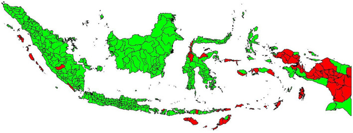 Figure 2
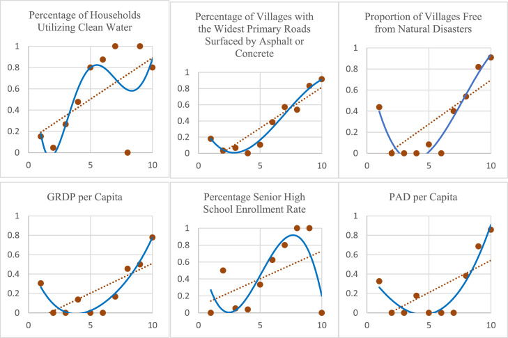 Figure 3
Peer Reviews
No public reviews on file for this paper yet. If you reviewed it on a platform where reviews are public (OpenReview, ICLR, NeurIPS, ICML), you can paste yours below so the community can read it here.
Videos
No videos yet. Explain this paper in a talk, walkthrough, or lecture? Add one.
Taxonomy
TopicsEconomic and Technological Innovation · Income, Poverty, and Inequality · Spatial and Panel Data Analysis
Specifications table
Subject areaMathematics and StatisticsMore specific subject areaStatistics; Nonparametric Regression; Categorical DataName of your methodFourier Series Nonparametric Binary Logistic Regression (FSNBLR)Name and reference of original methodFourier series function developed by Bilodeau (1992), M. Bilodeau, Fourier smoother and additive models, The Canadian Journal of Statistics 20 (1992) 257–269. https://doi.org/10.2307/3315313. Maximum likelihood estimation in the book of Hosmer, D. W., & Lemeshow, S. (2000), Applied Logistic Regression, 2nd Edition. United States of America, Canada. https://books.google.co.id/books?id=Po0RLQ7USIMC&lpg=PP1&pg=PP1#v=onepage&q&f=falseResource availabilityReturn on asset and its predictor variables data in 2021 of 232 districities/municipalities in East Indonesia could be accessed at the Indonesia publication data website (https://www.bps.go.id/id).
Background
Regional inequality remains a persistent challenge in many developing countries, including Indonesia. In particular, several districts across Eastern Indonesia continue to be classified as underdeveloped regions, characterized by deficiencies in infrastructure, education, economic activity, and access to basic services. This persistent disparity reflects Indonesia’s broader structural inequality, rooted in historical concentration of economic activities, fiscal resources, and infrastructure investment in Western Indonesia—particularly Java and Sumatra—while Eastern provinces such as Papua, Maluku, and East Nusa Tenggara have experienced slower structural transformation and limited access to development opportunities. Despite numerous government initiatives, including the Masterplan for Acceleration and Expansion of Indonesia’s Economic Development (MP3EI) and the Village Fund Program, these regions continue to lag behind due to geographic isolation, institutional capacity constraints, and uneven policy implementation.
Consequently, Eastern Indonesia provides a distinctive and policy-relevant context for analyzing the determinants of regional underdevelopment, where socioeconomic, geographic, and institutional factors intersect most sharply. Understanding the underlying determinants of underdevelopment is critical for informing targeted and effective policy interventions. However, the classification of regions as underdeveloped is often influenced by a complex interplay of multiple socioeconomic, geographic, and institutional factors. This complexity presents a significant modeling challenge, especially when conventional statistical models are insufficient to capture nonlinear or nonstandard relationships among variables.
Recent methodological advancements have led to the adoption of more flexible modeling approaches, including nonparametric regression frameworks. Among them, the Fourier Series Nonparametric Binary Logistic Regression (FSNBLR) model has emerged as a promising technique for modeling binary outcomes without imposing restrictive assumptions on the functional form of the relationship between predictors and the response variable [1]. FSNBLR builds upon the foundation of Nonparametric Binary Logistic Regression (NBLR), which was introduced to capture complex associations when the regression function is unknown or difficult to specify a prior [2]. Unlike traditional Binary Logistic Regression (BLR), which relies on the assumption of a linear link between predictors and the logit-transformed response, NBLR and its variants utilize data-driven smoothing techniques to estimate the regression function, thus offering greater modeling flexibility.
Generalized Additive Models (GAMs), provide a flexible framework by modeling the predictors' effects through smooth functions. However, GAMs often rely on spline-based smoothers and do not exploit the analytical advantages of orthogonal basis functions like Fourier series. Additionally, GAMs usually require careful selection of smoothing parameters and may not be optimized for periodic structures in the data [3]. The proposed FSNBLR addresses these limitations by introducing a Fourier basis within a nonparametric logistic regression setting, allowing for compact, interpretable representations of nonlinear patterns—particularly suitable for modeling periodic or oscillatory behavior.
Numerous smoothing techniques have been developed to operationalize nonparametric regression models, including the Spline estimator [4], Fourier Series estimator [5], Wavelet estimator [6], Kernel estimator [7], Local Polynomial Regression [8], and Multivariate Adaptive Regression Splines (MARS) [9]. Each method is suited to particular data structures and research contexts. For instance, splines are effective for data exhibiting localized variation based on predefined knots [4], while local polynomial regression has been employed to reduce bias and asymptotic variance in multivariate contexts [10]. Wavelet-based methods have demonstrated robustness in handling noisy data, particularly when the error component follows a Gaussian distribution [11,12].
Beyond the statistical literature, studies in development economics and spatial inequality have highlighted how disparities in fiscal capacity, human capital, and infrastructure investment contribute to persistent regional underdevelopment [[13], [14], [15]]. Empirical analyses such as those by [13] and [14] emphasize that Indonesia’s regional inequality is shaped by both structural and institutional dimensions, underscoring the need for data-driven modeling tools that can capture complex, nonlinear interdependencies. Integrating flexible statistical approaches like FSNBLR with regional policy research thus provides a stronger analytical foundation for identifying which socioeconomic variables most effectively inform spatially targeted development interventions.
Among these approaches, the Fourier Series estimator is particularly noteworthy for its ability to model periodic or repeating patterns in data [4]. It has demonstrated a favorable balance between model accuracy and computational efficiency in additive nonparametric regression frameworks [16]. Furthermore, it has shown strong performance in both univariate and multivariate settings [5,[16], [17], [18]]. Since its initial development in [5] and later expansion in [11], Fourier-based methods have been extended to semiparametric regression models [19], adapted for bivariate responses [20], and incorporated into various mixture-type modeling frameworks in both nonparametric [[21], [22], [23]] and semiparametric forms [24].
Despite its strengths, most applications of Fourier-based estimators have focused on continuous response variables [[25], [26], [27], [28]]. In practice, however, many empirical problems—such as classifying regions as underdeveloped or not—require models suited for binary or categorical outcomes. In response, researchers have explored nonparametric regression approaches for categorical data, including Local Likelihood Logit Estimation [29], decision tree-based methods [30], and B-spline-based techniques [31]. More recently, the FSNBLR model has been proposed as a nonparametric extension specifically tailored for binary outcomes [1].
However, existing applications of FSNBLR have primarily emphasized its descriptive capabilities and estimation flexibility, without incorporating the necessary inferential framework for hypothesis testing and formal assessment of predictor significance. This limitation hinders its utility in applied settings, where determining which predictors have statistically significant effects on binary outcomes is essential for evidence-based decision-making. Addressing this gap, the present study proposes a comprehensive inferential framework for the FSNBLR model, extending its functionality beyond estimation to support statistical inference. Specifically, the study introduces two hypothesis testing procedures: (i) simultaneous hypothesis testing via the Likelihood Ratio Test (LRT), which yields a test statistic asymptotically following a Chi-square distribution; and (ii) partial (individual) hypothesis testing via the Z-test, which evaluates the significance of individual predictors within the nonparametric structure.
In addition, this study formulates explicit research hypotheses grounded in socioeconomic development theory, positing that regions with higher fiscal capacity, better infrastructure, and greater human capital are less likely to be classified as underdeveloped, thereby linking the FSNBLR modeling framework with the theoretical underpinnings of regional inequality. To illustrate the practical utility of the proposed methodology, the FSNBLR model and its inferential extensions are applied to an empirical case study examining the determinants of regional underdevelopment in Eastern Indonesia. The analysis employs secondary data comprising one binary outcome variable (indicating underdeveloped status) and multiple predictor variables reflecting regional development indicators.
This study contributes to the literature in two key dimensions. Methodologically, it advances the FSNBLR framework by integrating formal statistical inference tools, enabling researchers to conduct hypothesis testing within a flexible, nonparametric binary regression context. Practically, it offers empirical insights into the drivers of regional underdevelopment, thereby providing a more rigorous and data-informed basis for regional policy planning and targeted development strategies in Indonesia. FSNBLR models such as this can provide classification results that correspond to data patterns and the significance of model parameters in identifying variables that can be prioritized by policymakers.
Method details
The development of the hypothesis testing procedure for the FSNBLR estimator involves several essential steps. First, the probability distribution of the binary response variable will be formulated. Based on this distribution, the FSNBLR model will then be constructed by incorporating the Fourier Series into the logistic regression framework. Subsequently, statistical inference will be established through the formulation of appropriate hypothesis testing procedures. In this context, simultaneous hypothesis testing will be conducted using the LRT, which evaluates the joint significance of the model parameters. Meanwhile, partial hypothesis testing will be carried out using the Wald test, which assesses the individual significance of each predictor variable. Conceptually, the use of the Fourier basis within the FSNBLR framework allows complex and nonlinear relationships to be expressed as a combination of smooth, periodic components. This is particularly suitable for socioeconomic phenomena that often exhibit cyclical or recurrent patterns—such as fiscal cycles, migration flows, or seasonal economic activities—where relationships between predictors and outcomes are rarely linear. By decomposing these relationships into interpretable harmonic terms, the FSNBLR model can capture nuanced variations in the data while remaining flexible and transparent, thereby making the methodology more accessible to researchers and policymakers beyond the field of statistics.
Probability distribution
Given , representing p predictor variables, the response variable was assumed to follow a Bernoulli distribution [1] with a probability distribution defined as:
where the success probability was given by:
and the failure probability by:
The probability function was defined in the Bernoulli probability mass function as follows:
FSNBLR estimator
FSNBLR model
The FSNBLR model is obtained [31] as follows:
In the model (2), , where , where , are the Fourier Series model parameters. Estimator of the model can be obtained using the Maximum Likelihood Estimation (MLE) method.
Likelihood functionl(θ)
The likelihood function is given, where
The likelihood function which is the multiplication of joint probabilities of random variables (1) is formulated as:
In practice, the parameter estimation in logistic regression is conducted by maximizing the log-likelihood function, which is obtained by taking the natural logarithm of Eq. (3). This transformation simplifies the optimization process, and the log-likelihood function is written as
Log-likelihood functionL(θ)
The likelihood function is expressed as follow:
The estimator derived by taking the partial derivatives of the log-likelihood function (4) with respect to each parameter , and equating these derivatives to zero.
Newton-Raphson iteration
The derivative of the log-likelihood function in Eq. (4) with respect to the parameters produces a complex system of equations that has no closed-form solution. This means that we cannot directly calculate the parameter values explicitly. Therefore, we need to use numerical methods to find the optimal parameter values. One method used is the Newton–Raphson method, which works iteratively to estimate the best values of the parameter vector . The iterative updating equation is given by:
where in Eq. (5) is the parameter estimate at the t-th iteration for until convergence. The vector is defined as:
The gradient vector contains the first-order partial derivatives of the log-likelihood function and is defined (6) as:
The Hessian matrix is composed of the second-order partial derivatives of the log-likelihood function and is organized (7) as follows:
Here, are the model parameters associated with the Fourier Series expansion within the nonparametric regression framework.
Estimatorθ^
From the Newton-Raphson iteration equation, the estimator is obtained when the convergence criterion is met:
Once this condition is satisfied (8), the final estimator vector is expressed as:
Based on the resulting estimator , the FSNBLR model (2) can be written as:
Here, are the estimated model parameters associated with the predictor variable , while correspond to those associated with the predictor variable . Where denotes the total number of predictor variables and represents the number of oscillation parameters and.
Hypothesis test for parameter model
The hypothesis testing for model parameters is divided into two types: simultaneous and partial. The simultaneous test is conducted using the Likelihood Ratio Test (LRT), while the partial test is conducted using the Wald test.
Simultaneous test
The simultaneous (overall) test evaluates the significance of the full set of model parameters in the model. The hypothesis form, parameter space, and statistic test are given as follows.
Hypothesis:
Parameter Spaces:
Under
Under population:
Theorem 1. Let be the parameter space for the population, and let ⊆ be the parameter space under the null hypothesis . Then, the test statistic used to test this hypothesis, called the Likelihood Ratio Test (LRT), is defined as follows:
Proof:
Lemma 1.1. The log-likelihood function (10) in Theorem 1 is approximated using a second-order Taylor series expansion around the MLE under the full model
With is the Fisher information matrix evaluated at .
Corollary 1.1.1. Because in Eq. (11) , the formulation in Lemma 1.1 could be defined as follows:
The log-likelihood function expanding around gives:
Corollary 1.1.2. Because , the formulation in Lemma 1.2 is given as follows:
Based on Lemma 1.1, combining (12) and (13), the LRT statistic in Theorem 1 becomes:
Suppose the parameters of the MLE estimator on the population are partitioned:
where,
Suppose the parameters of the MLE estimator at are partitioned:
where,
Lemma 1.2. Based on [32], the maximum likelihood estimator satisfies the asymptotic distribution:
and , then obtained
where,
and
Corollary 1.2.1. According to [33], the matrix can be written in the form of non singular matrices as follows:
with dan
The quadratic form in Eq. (14) can be decomposed into:
Corollary 1.2.2. Based on , then obtained:
The quadratic form in Eq. (15):
Corollary 1.2.3. Substitution :
then,
Substitute the results of (15) and (16) in Lemma 1.2 into Eq. (14), thus obtained:
Eq. (17) is simplified to
where,
and
Theorem 2. Under the null hypothesis , the distribution of the Likelihood Ratio Test (LRT) statistic asymptotically follows a chi-square distribution with degrees of freedom, where is the number of parameters per component and is the number of components.
Proof:
where
Thus it can be concluded
Theorem 3. Based on the statistical test defined in Theorem 1 and its distribution described in Theorem 2, the critical region for rejecting the null hypothesis at a significance level in the simultaneous hypothesis test of the parameters of the FSNBLR model is given by
where is the test statistic and is the upper quantile of the chi-square distribution with degrees of freedom.
Proof:
Reject if:
Partial test
The Partial (individual) tests are conducted to determine the significance of parameters individually. The hypothesis form, parameter space, and statistic test are given as follows.
Hypothesis:
For the main effect parameters , where
For the main effect parameters , where
Suppose the population MLE parameters are partitioned as:
Where:
Under the null hypothesis , the MLE parameters are partitioned as:
where:
Theorem 4. The test statistic used to evaluate a partial hypothesis, known as the Wald test, is given by
where is the estimated coefficient of the -th parameter, and is its estimated variance.
Proof:
The Wald test statistic is given by
Lemma 4.1. Based on normal asymptotic properties:
where, according to [34]:
Corollary 4.1.1 The element in Eq. (18) is the main diagonal element of the matrix
Form of Eq. (19) is equivalent to a standard normal test:
Corollary 4.1.2. Furthermore, with the same procedure, it can be done for hypothesis testing
Using the following test statistics:
with is the main diagonal element corresponding to of the matrix
Theorem 5. Based on the statistical test and its distribution described in Theorem 4, the critical region for rejecting the null hypothesis at a significance level in the partial hypothesis test of the parameters of the FSNBLR model is given by
where is the Wald test statistic, and is the upper quantile of the standard normal distribution.
Proof:
Since the statistical test given in Theorem 4, critical area for rejection of is obtained as follows:
Reject if:
Data collection
In applying the FSNBLR method, this study employs secondary data concerning the status of underdeveloped regions in Eastern Indonesia for the year 2021. The dataset includes one binary response variable, indicating whether a region is classified as underdeveloped or not. Then, six continuous predictor variables, obtained from various official sources such as Kementerian Desa, Pembangunan Daerah Tertinggal, dan Transmigrasi; Kementerian Dalam Negeri; Kementerian Pendidikan, Kebudayaan, Riset, dan Teknologi; Kementerian Keuangan; and Badan Pusat Statistik.
Research variabel
The data consists of one response variable ( ) and six predictor variables ( ). The variables are detailed in Table 1.Table 1. Variable description.Table 1. VariableNotationDescriptionUnitScaleResponse Status of Underdeveloped Regions0 = Developed 1 = UnderdevelopedNominalPredictor Percentage of Households Utilizing Clean WaterPercentRatio Percentage of Villages with the Widest Primary Roads Surfaced by Asphalt or ConcretePercentRatio Percentage of Villages without DisasterPercentRatio GDRB per CapitaThousand rupiahsRatio Percentage Senior High School Enrollment RatePercentRatio PAD per CapitaHundred thousand rupiahsRatio
Fig. 1 depicts a map of the spatial distribution of underdeveloped regions.Fig. 1. Distribution of underdeveloped regions in Indonesia in 2021.Fig 1
Based on Fig. 1, there are a total of 62 underdeveloped regencies across Indonesia. Of these, 55 are located in Eastern Indonesia, as detailed in Table 2.Table 2. List of underdeveloped areas in Eastern Indonesia 2021 based on presidential regulation No 63/2020.Table 2. RegionProvinceDistrictTotalPapuaPapua BaratManokwari Selatan, Maybrat, Pegunungan Arfak, Sorong, Sorong Selatan, Tambrauw, Teluk Bintuni, and Teluk Wondama.8 DistrictsPapuaAsmat, Boven Digoel, Deiyai, Dogiyai, Intan Jaya, Jayawijaya, Keerom, Lanny Jaya, Mappi, Memberamo Raya, Memberamo Tengah, Nabire, Nduga, Paniai, Pegunungan Bintang, Puncak, Puncak Jaya, Supiori, Tolikara, Waropen, Yahukimo, and Yalimo.22 DistrictsMalukuMalukuMaluku Tenggara Barat, Kepulauan Aru, Seram Bagian Barat, Seram Bagian Timur, Maluku Barat Daya, Buru Selatan6 DistrictsMaluku UtaraKepulauan Sula, Pulau Taliabu.2 DistrictsNusa TenggaraNTBLombok Utara1 DistrictNTTAlor, Belu, Kupang, Lembata, Malaka, Manggarai Timur, Rote Ndao, Sabu Raijua, Sumba Barat, Sumba Barat Daya, Sumba Tengah, Sumba Timur, and Timor Tengah Selatan.13 DistrictsSulawesiSulawesi TengahDonggala, Tojo Una-Una, Sigi3 DistrictsTotal11 Provinces55 Districts
Method validation
Descriptive analytics
Descriptive analysis is conducted to understand the characteristics of each predictor variables, as presented in Table 3.Table 3. Descriptive statistics of the predictor variables.Table 3. VariableMeanVarianceMinMax 81.28373.370.00100.00 69.14821.010.00100.00 55.90681.780.00100.00 55.203937.566.18589.11 63.89246.688.2594.92 46.931191.444.81281.79
Table 3 summarized the descriptive statistics for the six predictor variable used in the study, which represent characteristics of 232 regencies/cities in Eastern Indonesia. These variables are related to the classification of underdeveloped regions. All independent variables are correlated with the dependent variable [28], contain no missing values [29], and show no indication of multicollinearity [30]. The multicollinearity test is shown in the Table 4 below.Table 4. Multicolinearity test of the predictor variables.Table 4. VariableVIF 1.27 1.37 1.13 1.59 1.34 1.58
Based on Table 4, each predictor variable has a VIF value of <10, so it can be concluded that there is no multicollinearity between the predictor variables in the model. Each predictor variable is defined in accordance with Ministerial Regulation No 11/2020, which described as follows:
-
- Percentage of Households Utilizing Clean Water, is the proportion of households in a district/city that utilize clean water, calculated as the number of such households relative to the total, expressed as a percentage.
-
- Percentage of Villages with the Widest Primary Roads Surfaced by Asphalt or Concrete, is calculated by dividing the number of villages with asphalt or concrete as the main road surface type by the total number of villages in the district.
-
- Proportion of Villages Free from Natural Disasters*,* is the ratio of villages that have not experienced natural disasters (e.g., floods, earthquakes, droughts) within the past three years, expressed in percentage terms relative to the total number of villages.
-
- GRDP per Capita, refers to the Gross Regional Domestic Product measured on a per-person basis within a district.
-
- Percentage Senior High School Enrollment Rate, is the proportion of individuals aged 16–18 currently enrolled in senior high school compared to the total population in that age group, presented as a percentage.
-
- PAD per Capita, is the district’s own-source revenue divided by its total population, indicating the fiscal capacity per person.
To explore the potential nonlinear relationships between each predictor and underdeveloped status, we constructed scatterplots of grouped data against the proportion of underdeveloped regions. These are presented in Fig. 2.Fig. 2. Scatterplots comparing multiple data groups against proportion of underdeveloped regions per group.Fig 2
From Fig. 2, it is evident that the probability of being underdeveloped tends to increase with each predictor variable, following a repetitive and ascending pattern. This supports the suitability of modeling the data using a FSNBLR approach. Accordingly, this study proceed by implementing both the Binary Logistic Regression (BLR) and FSNBLR models. The parameter estimation and their statistical significance are discussed in the following section.
BLR model
The BLR model is specified as follows.
where, is the intercept, and are the slope coefficients corresponding to the predictor variables.
Parameter estimation in BLR model
Based on the estimation output, the fitted BLR model for underdeveloped regions data is given by:
Significant parameter in BLR model
The significance test for each parameter in the model is shown in Table 5.Table 5. Significant parameter in BLR model.Table 5. ParametersEstimationsStd. Errorz valuePr(>|z|)Decision 3.62761.53682.360.0183reject −0.00850.0125−0.6760.4993fail to reject −0.04380.0096−4.5550.000005reject 0.01280.00871.4560.1455fail to reject −0.01210.0105−1.1480.2509fail to reject −0.00720.0180−0.40.6894fail to reject −0.03010.0140−2.1460.0319reject
The results in Table 5 indicated that only (percentage of villages with asphalt/concrete roads) and (PAD per capita) are statistically significant at the 5 % significance level. Therefore, these two variables significantly influence the probability of a region being classified as underdeveloped.
The refined model using only statistically significant parameters is:
Detailed parameter estimation for the best BLR model using only statistically significant parameters provided in Table 6.Table 6. Parameter estimation of the best BLR model.Table 6. ParametersEstimationsStd. Errorz valuePr(>|z|)Decision 3.44520.65155.2880.00000012reject −0.04900.0079−6.1770.000000000653reject −0.04140.0109−3.8000.000145reject
Based on Table 6, this model suggests that higher percentages of asphalt/concrete road coverage and greater PAD per capita are associated with a lower probability of a region being underdeveloped.
FSNBLR model
Selection of optimal parameters
The oscillation parameters in the FSNBLR model were determined through the minimization of the Akaike Information Criterion (AIC). In order to avoid overfitting and to ensure the interpretability of the model, the number of oscillation parameters were limited. Using an R algorithm, the AIC values for various combinations of oscillation parameters were calculated and are summarized in Table 7.Table 7. Minimum AIC values for each number of oscillation parameter.Table 7. Maximum Parameter OscillationCombination (K)AIC (K) 111111169.3606 121111169.1771 321111168.4055
Based on Table 7, the model with oscillation parameters yields the smallest AIC and is therefore selected as the optimal FSNBLR model.
Parameter estimation in FSNBLR model
The FSNBLR model (25) can be expressed as:
Detailed parameter estimation are provided in Table 8.Table 8. Parameter estimation of the FSNBLR model.Table 8. ParametersEstimationsParametersEstimations 4.0393 0.0115 0.0005 −0.4500 0.0946 −0.0092 0.4071 −0.3481 −0.5541 −0.0117 −0.0582 0.3969 −0.5454 −0.0338 −0.5136 0.0831
Significant parameter in FSNBLR model
Significance tests for each parameter are summarized in Table 9.Table 9. Significant test of parameters in the FSNBLR model.Table 9. ParametersEstimationsStd. Errorz valuePr(>|z|)Decision 4.03931.65362.4430.0146reject 0.00050.01290.0400.9685fail to reject 0.09460.32220.2940.7689fail to reject 0.40710.33771.2050.2280fail to reject −0.55410.3123−1.7740.0760fail to reject −0.05820.0121−4.7870.000001reject −0.54540.3469−1.5720.1160fail to reject −0.51360.3463−1.4830.1381fail to reject 0.01150.00951.2120.2254fail to reject −0.45000.3339−1.3480.1778fail to reject −0.00920.0085−1.0850.2779fail to reject −0.34810.3401−1.0230.3061fail to reject −0.01170.0207−0.5670.5706fail to reject 0.39690.34311.1570.2472fail to reject −0.03380.0143−2.3600.0183reject 0.08310.32160.2590.7959fail to reject
Based on Table 9, the results indicate that only (percentage of villages with asphalt/concrete roads) and (PAD per capita) are statistically significant.
The best FSNBLR model with significant parameters and oscillation parameters is:
Detailed parameter estimation for the best FSNBLR model using only statistically significant parameters provided in Table 10.Table 10. Parameter estimation of the best BLR model.Table 10. ParametersEstimationsStd. Errorz valuePr(>|z|)Decision 3.76950.71875.2450.00000015reject −0.05390.0089−6.0340.0000000016reject −0.47830.3184−1.5020.1330fail to reject −0.51510.3161−1.6290.1032fail to reject −0.04400.0113−3.8820.00010reject 0.23730.30200.7860.4319fail to reject −0.01050.2882−0.0360.9709fail to reject −0.66040.3356−1.9680.0490Reject H_0_
Based on Table 10, this implies that the status of underdeveloped regions is significantly influenced by the percentage of villages with asphalt/concrete roads and PAD per capita, including their oscillatory effects captured by the Fourier series components.
Comparison of BLR and FSNBLR
Model selection for classification based on deviance value
The preferred regression model is the one with the lowest deviance value. The results obtained from the deviance statistical test are presented in Table 11.Table 11. Deviance value comparison between models.Table 11. MethodsDeviance ValuesBLR157.6297FSNBLR147.4715
Based on Table 11, the deviance value for the FSNBLR (147.4715) was smaller than that for the BLR (157.6297). Therefore, the FSNBLR model is the best model for data on the status of underdeveloped regions because has the smallest deviance value.
Model selection for classification based on AUC and Press’s Q value
The chosen FSNBLR model exhibited the highest AUC or the lowest Press's Q value. The results of the classification test are presented in Table 12.Table 12AUC and Press’s Q value comparison between models.Table 12. MethodsAccuracySensitivitySpecificityAUCPress’s QChi SquareBLR82.32 %92.65 %49.09 %70.87 %96.982796.4927FSNBLR84.05 %93.22 %54.54 %73.88 %107.603496.4927
Table 12 indicates that the FSNBLR model achieved a higher AUC value (73.88 %) compared to the BLR model (70.87 %). Furthermore, the greater Press’s Q value for FSNBLR (107.6034) suggests a stronger classification capability and a higher likelihood of rejecting the null hypothesis.
Summary
Based on the hypothesis testing and model comparisons that had been conducted, the BLR model identified variables (Percentage of Villages with Asphalt/Concrete Road Surface) and (PAD Per-Capita) as significant parameters. This is also the same as the FSNBLR model, which found and to be significant. The FSNBLR model with significant parameters for categorical data is followed:
The FSNBLR model provided better fit and classification performance than the BLR model, as shown by higher AUC, accuracy, sensitivity, and specificity values. Therefore, it was concluded that the FSNBLR model was more suitable for predicting the status of underdeveloped regions in Eastern Indonesia in 2021. The results shown that the significant parameters are the Percentage of Villages with Asphalt/Concrete Road Surface and PAD Per-Capita. These two variables should also be considered as key elements in planning development policies to reduce regional underdevelopment.
A higher percentage of villages with asphalt or concrete road surfaces indicates better transportation infrastructure, which plays a critical role in supporting economic activities. Good road conditions facilitate the smooth distribution of goods and services, ease access to markets, reduce travel time and costs, and improve connectivity between regions. This, in turn, stimulates economic growth and development in other sectors such as agriculture, trade, and education.
Meanwhile, a higher PAD per capita reflects the fiscal capacity of a region. With greater locally-generated revenue, local governments have more flexibility and resources to fund strategic programs—such as infrastructure development, education, health services, and economic empowerment initiatives. This financial capacity is essential in supporting comprehensive and sustainable efforts to uplift underdeveloped areas. Therefore, strengthening road infrastructure and increasing PAD should be prioritized as part of integrated regional development strategies.
These findings have direct socioeconomic and policy implications. The statistical significance of infrastructure and fiscal capacity variables highlights the need for development strategies that prioritize equitable budget allocation toward road improvement and local revenue enhancement. In practical terms, this means that national and regional governments should integrate infrastructure investment and fiscal capacity-building programs into a coordinated regional development agenda—ensuring that remote districts in Eastern Indonesia receive both physical connectivity and financial autonomy to sustain local growth. By translating the FSNBLR results into actionable policy priorities, the study bridges quantitative modeling with real-world decision-making in regional development planning.
Nevertheless, the study acknowledges several limitations, including potential data heterogeneity, temporal instability, and challenges in parameter interpretability. Future research is encouraged to extend the FSNBLR framework to panel and spatial data structures, or to integrate it with AI-based prediction techniques, to enhance robustness and capture the evolving dynamics of regional inequality. Furthermore, extending the FSNBLR framework to account for spatial dependencies or uncertainty quantification via Bayesian inference represents another promising direction to improve model reliability and applicability in complex socioeconomic data settings. Overall, the FSNBLR framework provides a strong methodological foundation for future interdisciplinary research that links quantitative modeling, spatial analysis, and policy design—supporting more adaptive and evidence-based regional development planning in Indonesia and comparable developing economies.
Limitations
-
- The method used to select the optimal oscillation parameters was the smallest AIC.
-
- The number of oscillation parameters (k) used in the Fourier series in this study is k = 1, 2, and 3
-
- The estimation method used in the Fourier series nonparametric regression model of categorical data is Maximum Likelihood Estimation (MLE).
-
- The cutoff threshold for classifying the results 0 and 1 from the probability prediction used is 0.5.
-
- The hypothesis testing method used is the Maximum Likelihood Ratio Test (MLRT).
-
- The confidence interval method used is Pivotal Quantity.
-
- The best model-comparison method uses the classification test.
-
- The data used are secondary data from Eastern Indonesia (West Nusa Tenggara, East Nusa Tenggara, West Kalimantan, Central Kalimantan, South Kalimantan, East Kalimantan, North Kalimantan, North Sulawesi, Central Sulawesi, South Sulawesi, Southeast Sulawesi, Gorontalo, West Sulawesi, Maluku, North Maluku, West Papua, and Papua).
-
- Ignoring dependencies between observations, so that observation groups can be obtained from the smallest to largest sequence of values.
-
- Continuous variables do not exhibit multicollinearity.
Ethics statements
The data we use in this research are secondary data that we collected from publications of each province in Eastern Indonesia. The data is available on request.
CRediT authorship contribution statement
Muhammad Zulfadhli: Conceptualization, Methodology, Software, Writing – original draft, Visualization. I Nyoman Budiantara: Conceptualization, Methodology, Writing – review & editing, Validation, Supervision. Vita Ratnasari: Conceptualization, Methodology, Writing – review & editing, Validation, Supervision. Afiqah Saffa Suriaslan: Conceptualization, Methodology, Writing – review & editing, Validation, Supervision. Risdiana Chandra Dhewy: Conceptualization, Methodology, Writing – review & editing, Validation, Supervision.
Declaration of competing interest
The authors declare that they have no known competing financial interests or personal relationships that could have appeared to influence the work reported in this paper.
The reference list from the paper itself. Each links out to its DOI / PubMed record.
- 1Zulfadhli M.Budiantara I.N.Ratnasari V.Nonparametric regression estimator of multivariable fourier series for categorical data Methods X 11202410298310.1016/j.mex.2024.102983 PMC 1182909439959887 · doi ↗ · pubmed ↗
- 2Harrell F.E.Jr.Regression Modeling Strategies: With Applications to Linear Models, Logistic and Ordinal Regression, and Survival Analysis 2nd ed.2015 Springer New York 10.1198/tech.2003.s 158 · doi ↗
- 3Hastie T.J.Tibshirani R.J.Generalized Additive Models 1990 Chapman and Hall/CRC London
- 4Eubank R.L.Spline Smoothing and Nonparametric Regression 1998 Marcel Dekker New York
- 5Li L.Nonlinear Waveled-Based Nonparametric Curve Estimation With Consored Data and Inference on Long Memory Processes 2002 Pro Quest Information and Learning Company, United States Code
- 6Okumura H.Naito K.Non-parametric kernel regression for multinomial data J. Multivar. Anal.97200620092022
- 7Sua L.Ullah A.Local polynomial estimation of nonparametric simultaneous equations models J. Econom.1442008193218
- 8Yasmirullah S.D.P.Otok B.W.Purnomo J.D.T.Prastyo D.D.Modification of multivariate adaptive regression spline (MARS)J. Phys.1863202101201710.1088/1742-6596/1863/1/012078 · doi ↗