There are no alternative hypotheses in tests of null hypotheses
Denis Cousineau

TL;DR
This paper clarifies that null hypothesis testing involves only one hypothesis, not two, and explains how this misconception has led to misinterpretations in statistical methods.
Contribution
The paper identifies a fundamental misconception in NHST teaching and introduces dual hypotheses statistical testing as a distinct procedure.
Findings
Null hypothesis statistical testing does not involve an alternative hypothesis.
Procedures with power analysis and type-II thresholds are part of a different inferential framework.
The confusion stems from applying Aristotle's excluded middle to empirical science.
Abstract
Null hypothesis statistical testing (NHST) is typically taught by first posing a null hypothesis and an alternative hypothesis. This conception is sadly erroneous as there is no alternative hypothesis in the NHST. This misconception generated erroneous interpretations of the NHST procedures, and the fallacies that were deduced from this misconception attracted much attention in deterring the use of NHST. Herein, it is reminded that there is just one hypothesis in these procedures. Additionally, procedures accompanied by a power analysis and a threshold for type-II errors are actually a different inferential procedure that could be called dual hypotheses statistical testing (DHST). The source of confusions in teaching NHST may be found in Aristotle's axiom of excluded middle. In empirical sciences, in addition to the falsity or veracity of assertions, we must consider the…
Genes, proteins, chemicals, diseases, species, mutations and cell lines named across the full text — each resolved to its canonical identifier and authoritative record.
Click any figure to enlarge with its caption.
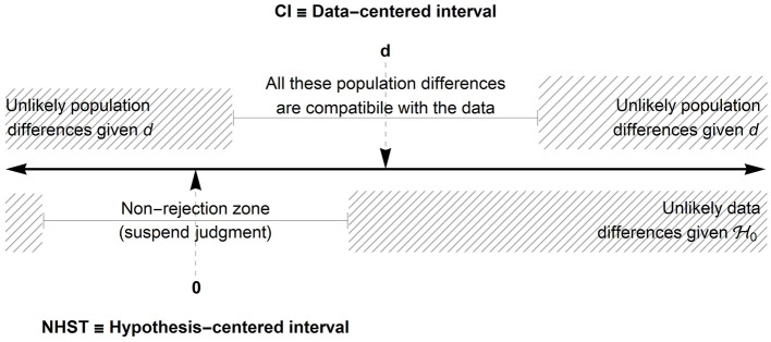 Figure 1
|
|
|
|
|
|---|---|---|---|
| Hypothesis |
|
| |
| Error Control | type I: α | type I: α | type II: β |
| Possible decisions |
- —Social Sciences and Humanities Research Council of Canada10.13039/501100000155
- —Natural Sciences and Engineering Research Council of Canada10.13039/501100000038
Peer Reviews
No public reviews on file for this paper yet. If you reviewed it on a platform where reviews are public (OpenReview, ICLR, NeurIPS, ICML), you can paste yours below so the community can read it here.
Videos
No videos yet. Explain this paper in a talk, walkthrough, or lecture? Add one.
Taxonomy
TopicsMeta-analysis and systematic reviews · Statistical Methods in Clinical Trials · Hemodynamic Monitoring and Therapy
Introduction
It is very common to see the description of a t test with the following hypotheses:
These are the very first step shown and introduced when teaching this procedure, and already, half of it is wrong! It is then no surprise that so many misconceptions and so-called fallacies were derived from this incorrect conceptualization (starting with Rozeboom, 1960; also see Greenland et al., 2016; Trafimow, 2003, among many others).
This misconceptualization is general and is also present when teaching ANOVAs (“ for at least one pair i, j”) and other null hypothesis statistical tests (NHST). It is vastly widespread, being found in many statistical teaching aids and textbooks to many disciplines (to name a few, Field, 2009; deGroot and Schervish, 2012; Gravetter and Wallnau, 2017; Agresti, 2021; for a review, see Cassidy et al., 2019), it has a long history (already Fisher, 1935, discusses it) and is enduring (Lytsy et al., 2022), affecting students and their educators equally as well as statisticans (Haller and Krauss, 2002; Lecoutre et al., 2003).
Fisher (1925), who created or formalized many of these procedures, never appealed to an alternative hypothesis. He made his view clear, stating that “Every experiment may be said to exist only in order to give the facts a chance of disproving the null hypothesis”. (Fisher, 1935, p. 16; also see Lehmann, 2011), adopting a stance similar to Popper's falsificationism (Popper, 1963). The alternative hypothesis was invented by Neyman and Pearson (1928) for a different purpose (see last section); Fisher disavowed its usage (Fisher, 1935; Denis, 2004; Cohen, 1992b).1
In what follows, we first summarize a typical null hypothesis test procedure, the well-known t test, highlighting what are the necessary ingredients to perform this test. As will be seen, nowhere is information from a so-called alternative hypothesis needed. We next conjecture that the source of the error is to be found in Aristotle's conception of logic as being two-valued only. We argue that adopting an approach that eliminates alternative hypotheses would enhance considerations given to the notion of evidence-based inferences. Third, we derive common errors that arose from this misconception. All these errors, occurring in undergraduate students and well-trained researchers, would simply not exist if the alternative hypothesis had never been taught. Finally, as promoted by Cohen (1969, 1992a), it is possible to test two hypotheses, but the resulting framework is quite different from the tests of null hypotheses; we end by clarifying the distinctions between the two procedures.
The ingredients of a null hypothesis statistical test
To illustrate the absence of an alternative hypothesis in NHST, we comment on a single instance, the t test on two independent groups. The conclusion reached at herein is the same for any other test of a null hypothesis such as the ANOVAs. The t test can be derived in many ways; herein, we proceed via a model comparison approach. Let us define the following two models, the second being a restricted version of the first:
in which Xij denotes a realization of the dependent variable in group i (i = 1 or 2) for participant j (j = 1, …, ni), denotes a normal distribution with parameters μ and σ. In the more general model Ma, μ_i_ are allowed to differ between the two groups, but in the restricted model Mb, both μ_1_ and μ_2_ are restricted to be equal (noting μ without a subscript). In both groups, the standard deviation is the same (from the so-called homogeneity of variance assumption).
As the various μs are parameters, they require estimators. The ones that maximize the likelihood of the models,
where f is the PDF of the normal distribution, are the means in each group (μ_i_ estimated by for Ma) or the grand mean (μ estimated by for Mb). The results are denoted as and .
Minus twice the log of the maximized likelihood ratio (λ^*^) simplifies to the usual t statistic squared,
where sp is the pooled standard deviation and ñ is the harmonic mean of the two groups' sample sizes.
The likelihood ratio test (Wilks, 1938) states that minus twice the log ratio of two likelihoods for maximally likely models, one being a restricted version of the other, follows a chi-square distribution with degrees of freedom given by the difference in the number of maximized parameters in both models (here 2 − 1 = 1). Wilks's result is asymptotic (infinitely large n); Fisher (1925) generalized this result for small n with the F distribution. As known, the square root of variates following the F distribution with 1 degree of freedom at the numerator is a t distribution. Previously, Gossett (Student, 1908) found the t distribution using an independent approach.
In summary, this test compares the model where the means are as observed in both groups relative to the model where the mean is the same in both groups. The second model will necessarily have a poorer fit, but the critical question is to assess how detrimental the restriction is. Using a decision threshold α, it is possible to determine limits beyond which the restriction is too severe to be plausibly maintained.
The final result of this procedure is a rejection region surrounding the null and delimited by boundaries tleft = tn1+n2−2, α/2 and tright = tn1+n2−2, 1−α/2 whose extent is based on the decision threshold α and the sample size n. Nowhere are the specifications provided by the alternative hypothesis used in this whole procedure. Therefore, why postulate one?
The source of the confusions
The reason why so many students, researchers and teachers alike feel an urge to add an alternative hypothesis may be related to how logical statements are conceived. For many, a statement is either true or false, but no other states are conceivable. This conception dates back to antiquity. For example, Aristotle assumed that if two propositions are in opposition (i.e. where one proposition is the negation of the other, that is, mutually exclusive), then one must be true, and the other must be false (Aristotle, ca. 340 BC; English translation 2015). This came to be known as the axiom of the excluded middle.
This position may be sensible in mathematics; however, it poorly fits how the acquisition of knowledge—and science generally speaking—progresses. In the empirical sciences, it is not possible to prove that a theory is true or false. Thus, the intrusion of the axiom is dubious. In an empirical investigation, a sample is gathered and evaluated with respect to a status quo ante position, that is, a position that lacks a novel effect. This evaluation could provide little support for this no-effect position where the strength of this misfit is assessed, for example, with a p value. However, a nonextreme p value says nothing with regard to the status quo. Asked “Should we abandon the status quo?”, the correct answer in this case would be “We still do not know” because the sample does not provide strong-enough evidence.
In this view, the acquisition of knowledge is build from a preliminary state of unknowing. When rejecting the null, we decide to leave this state for a state excluding the null. On the other hand, not rejecting the null means that we remain in the state of unknowing. In Howell's words, we must suspend any judgment (Howell, 2010, p. 94).
This principle summarizes evidence-based research. Either the evidence is sufficient to exclude the null or it is inconclusive. Here, an inconclusive state does not mean that we move to a state including the null state; rather, the state of knowledge is stalled and unchanged, because of a lack of evidence.
Alternatively, confusion may have to do with the modus tollens. For the premisse “If the data are congruent with , then p>0.05”, we can conclude that “The data are not congruent with ” when “p is not larger than 0.05”. However, when is defined as the negation of , then the conclusion rapidly becomes “The data are congruent with ”. Sadly, many things are wrong here, including the premisse. It should read “If the population is congruent with , then p>0.05 most of the time”.
Consequences of postulating an alternative hypothesis
Assuming the existence of an alternative hypothesis has consequences, and these consequences are all negative. Four are hightlighted here.
Accepting the null
Statistics instructors spend numerous hours dispelling this incorrect conclusion. Why is it so recurrent and so difficult to atone? The problem of how to interpret a nonrejected null hypothesis has plagued students in statistics courses for over 75 years (Howell, 2010, p. 93). Despite numerous discussions and warnings (among others, Lecoutre et al., 2003), a recent survey suggests that accepting the null is still widely performed by researchers (Edelsbrunner and Thurn, 2024).
The persistence of this error may be related to a framing effect: By introducing two propositions that are in opposition, we place the student in a logic mode of thinking. In this mode, if A is not true, then its opposing statement has to be true. In this mode, what is a nonacceptation of the alternative if not an acceptance of the null?
Not teaching would avoid this dichotomized mode of thinking and more easily let the concept that if cannot be rejected, it is because the data are inconclusive (see Dushoff et al., 2019, for a similar argument).
Misinterpreting the p value
Many come to the false conclusion that the p value is the probability of the null hypothesis (Cohen, 1992b). When the only visible outcome of the procedure is with regard to rejecting the null or not, the probability of the null is the only thing that comes to mind. If the NHST is presented without an alternative hypothesis, with a focus on obtaining evidence for rejecting the null hypothesis, then the probability of the evidence should come to mind, which is much closer to the true definition of the p value. The probability of the evidence places the focus on the data observed. Consequently, realizing that it is conditional on the null model assumed is a simple extension: the p value is the probability of the evidence assuming the null model.
Appealing to a possible type-II error
It is frequent to read research articles in which the authors report a nonsignificant result and then appeal to a possible type-II error (deciding not to reject the null when it is false). The correct conclusion being that the data are inconclusive, how can a lack of conclusion be an erroneous conclusion?
Appealing to a possible type-II error shows that the outcome of the procedure is poorly understood. Many other possible interpretations are possible. For example, (i) the sample size may be too small to detect anything (Cohen, 1992a); (ii) the true effect might be non-null but so small that the experiment lacks the necessary sensitivity (Lykken, 1968); and (iii) the controls exercized on the sampled groups may be insufficients to bring forward the difference (Wilson Van Voorhis and Morgan, 2007).
A properly calibrated statistical procedure comes with a certain guarantee: the probability of error when a decision is made has a knwown magnitude. In NHST, this probability is adjusted with the decision threshold α. In NHST, there is no way to know the probability of a type-II error as there is no decision threshold for errors of this type (this second probability is usually represented with β in other inferential frameworks, e.g., the non-equivalence tests and the dual-hypotheses tests; see next section).
A type-II error may occur when a decision is endorsed. Not endorsing a position cannot result in an error. Suspending our jugdment is not a judgment. NHST is not designed to provide support to the null hypothesis. Hence, if the purpose is to support the null, do not use a NHST procedure.
Overinterpreting confidence intervals
The confidence intervals are often conceived as alternative but equivalent representations of the NHST. This is not exactly the case. A confidence interval of a difference for example provides a zone in which all the population differences of size δ would not be rejected, if tested in a null hypothesis of the sort . This zone can be called a compatibility zone (Amrhein et al., 2019; Wasserstein and Lazar, 2016). Population differences outside this zone are said to be incompatible with the observed data whose difference is .
One way to illustrate the two approaches is to realize that the confidence intervals provides an interval centered on the observed statistic whereas NHST offers an interval centered on the null hypothesis. Figure 1 illustrates these two intervals.
Illustration of an interval based on the null hypothesis (lower half) and an interval based on the observed difference d (upper part). Note: 0 is the population difference hypothesized in H0; d is the observed difference. In this illustration, the observed difference d is located in the rejection zone so the null hypothesis H0 can be rejected with a given decision level α.
When 0 (or the value hypothesized by ) is included in the confidence interval, it does not mean that we accept . It means that is one possible interpretation compatible with the data.
With confidence intervals, assigning a probability to a specific population parameter value is not possible. Therefore, accepting a specific population value is unwarranted because it is not possible to know the risk of an error to such a conclusion.
Sadly, many erroneous interpretations of confidence intervals abound among trained researchers and authors (Hoekstra et al., 2014). To be correct, the confidence interval must be conceptualized as a compatibility interval whereby differences outside the interval are incompatible with the observed data (Amrhein et al., 2019).
Is the alternative hypothesis a questionable research practice?
Questionable research practices were first defined by Ioannidis (2005). Collectively, these practices deteriorate the quality and credibility of research even if most of the time, the authors are unaware of their presence (Sijtsma, 2016). Flake and Fried (2020) argued for the importance of defining the construct used in questionaires. For example, a researcher should be able to answer questions such as What is your construct?, Why did you select this measurement? Although they designed the questions to questionnaires and their items, the same questions can be made with respect to the framework used for statistical inference: Why did you choose the NHST? and Why did you select the p*-value for your inference*? We could also add: How will you interpret that measure? In the absence of a clear line of interpretation supported by the framework, unfounded conclusions can be drawn, reducing the credibility of the tool used.
Power planning with NHST
Cohen (1969, 1992a,b), for many decades, observed that typical sample sizes in the social sciences where too often very small and consequently had little chance of rejecting the null hypothesis when it is false. This notion is call the statistical power of a design. To improve statistical power, he suggested that, during the planification stage, experimenters settle on one specific alternative hypothesis (e.g., for a one-directional test, or for a two-directional test; Δ≠0). Using this specific alternative, it is then possible to find a sample size such that –simultaneously– the probability of being outside the rejection zone of when it is true is a desired α level and the probability of being inside the rejection zone of when is true is a desired 1−β level (Cohen suggested using α = 0.05 and 1−β = 0.80). Once the sample size is set, Cohen would simply forget and continue with a regular NHST.
This approach is now commonly used in planning a design and has been very efficient in improving statistical power in the psychological and social sciences. It was inspired by the Dual hypotheses testing used in Neyman and Pearson, as seen below, and became a practical approach with the advent of noncentral distributions that were being discovered between the 1930s and the 1950s (e.g., Johnson and Welch, 1940).
Dual hypotheses statistical testing (DHST)
Neyman and Pearson (1928, 1933) considered an approach with two hypotheses. In this view, the alternative hypothesis is likewise a pointwise hypothesis, such that
The analyst must set a decision threshold α but also a decision threshold β. With this dual testing procedure, it is possible to reject , which says that evidence favors over and vice versa, it is possible to reject , which says that evidence favors over . Thus, can be accepted (Cohen, 1992b, p. 1308).
As a consequence, there is a possibility that a type-II error occurs when is rejected. It is also possible that a type-I error occurs when rejecting . Both error probabilities are adjusted to acceptable levels by setting α and β as desired. As suggested by the features of these inferential frameworks listed in Table 1, the DHST can be seen as a combination of NHST and non-equivalence hypothesis testing (Lakens et al., 2018).
Conclusion
Discussing with colleagues that there is no alternative hypothesis in NHST, many simply replied that as long as it helps the student understand the logic of statistical testing, teaching is inconsequential. Instead, we believe that many errors and misconceptions arise from the erroneous teaching of and that the students would be better without this concept. It it more appropriate to say that after a non-significant result, “we still don't know whether should be abandoned or not”, or “we must suspend our judgment until more decisive data are collected” (Jones and Tukey, 2000, p. 412).
As argued in this text, the many errors that are triggered by the erroneous presence of an alternative hypothesis in the NHST are actually language errors built on cognitive limits and approximate guesses from the learners. These errors could be reversed by providing a deeper understanding of the NHST's inner gears and meanings (e. g., Wasserstein and Lazar, 2016) or teaching Bayesian statistics in parallel (Lecoutre, 2006). However, it seems easier to just obliterate the source of the error: there is no alternative hypothesis.
We urge instructors of statistics to stop including an alternative hypothesis when presenting NHST. It is possible, see Howell, 2010 (or in french, Cousineau, 2009). This error is creating considerable harm and confusion, and taken literally, results in fallacies. Removing a single line (“ ”) which is not used anywhere, will minimize or eliminate the many misconceptions that are triggered by it.
The reference list from the paper itself. Each links out to its DOI / PubMed record.
- 1Agresti A. (2021). Statistical Methods for the Social Sciences (5th Edition). London: Pearson.
- 2Amrhein V.Greenland S.Mc Shane B. (2019). Scientists rise up against statistical significance. Nature 567, 305–307. 10.1038/d 41586-019-00857-930894741 · doi ↗ · pubmed ↗
- 3Aristotle (2015). Peri Hermeneias [on interpretation]. Adelaide: Adelaide University.
- 4Cohen J. (1969). Statistical Power Analysis for the Behavioral Sciences. London: Academic Press.
- 5Cohen J. (1992 a). A power primer. Psychol. Bullet. 112, 155–159. 10.1037//0033-2909.112.1.15519565683 · doi ↗ · pubmed ↗
- 6Cohen J. (1992 b). Things I have learned (so far). Am. Psychol. 45, 1304–1312. 10.1037//0003-066X.45.12.1304 · doi ↗
- 7Cousineau D. (2009). Panorama des Statistiques pour les Sciences Humaines. Bruxelles: de Boeck Université.
- 8de Groot M. H.Schervish M. J. (2012). Probability and Statistics (4th edition). London: Addison-Wesley.