The Roles of Space and Food‐Web Complexity in Mediating Ecological Recovery
Klementyna A. Gawecka, Matthew A. Barbour, James M. Bullock, Jordi Bascompte

TL;DR
This study shows how the layout of habitats and food-web complexity affect the recovery of species during large-scale ecological restoration.
Contribution
The paper reveals how spatial configuration and food-web complexity jointly influence ecological recovery in restoration efforts.
Findings
The spatial arrangement of communities affects colonization of empty habitat patches.
Food-web complexity slows recovery of lower trophic levels but may have reduced effects at higher complexity.
Population recovery in populated patches is not influenced by spatial configuration.
Abstract
Landscape‐scale ecological restoration is a key strategy for halting and reversing biodiversity decline. However, ensuring the long‐term sustainability of restoration efforts requires guiding the recovery of complex ecological systems with many interdependent species at a landscape scale. Due to these challenges, our understanding of recovery trajectories remains limited. Using metacommunity models and experiments, we explore how the spatial configuration of communities and food‐web complexity jointly influence species recovery at different spatial scales. We find that the number and spatial placement of communities affect the colonisation of empty habitat patches, but do not influence population recovery in patches where communities are introduced. Food‐web complexity reduces the recovery of lower trophic levels. However, this negative effect may be partially mitigated at higher levels…
Genes, proteins, chemicals, diseases, species, mutations and cell lines named across the full text — each resolved to its canonical identifier and authoritative record.
Click any figure to enlarge with its caption.
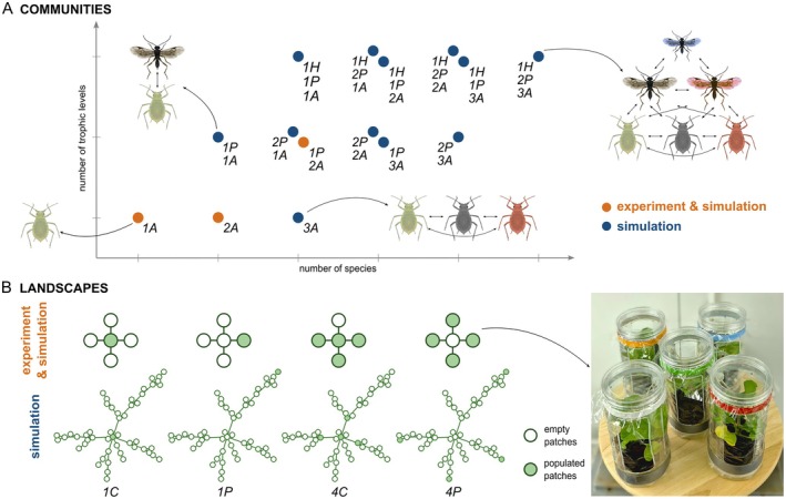 FIGURE 1
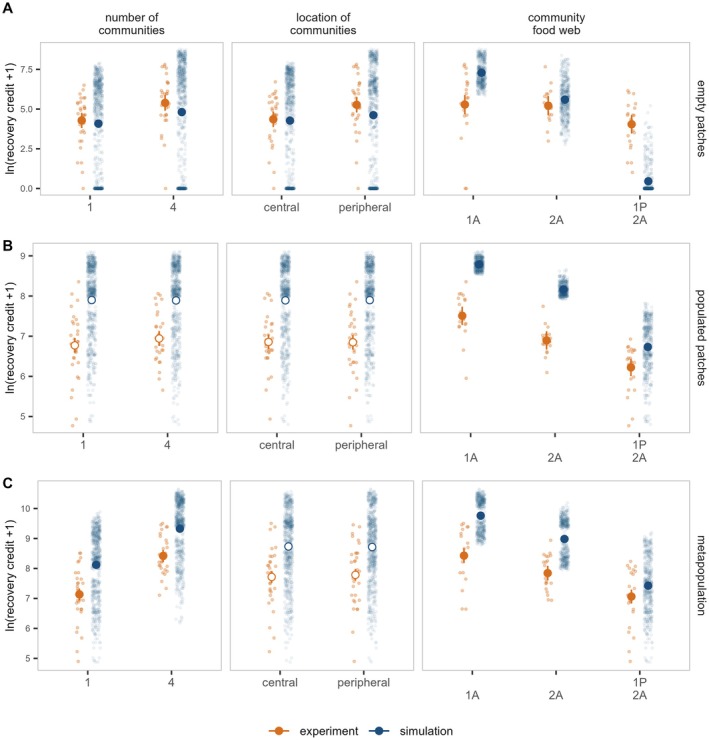 FIGURE 2
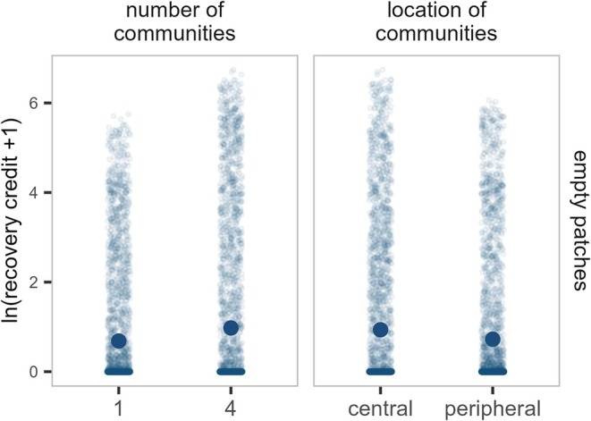 FIGURE 3
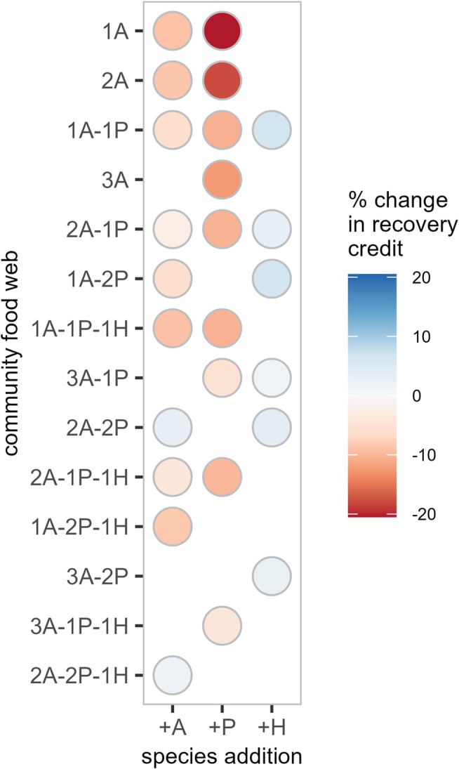 FIGURE 4
- —HORIZON EUROPE Marie Sklodowska‐Curie Actions10.13039/100018694
- —Fonds de recherche du Québec ‐ Nature et technologies10.13039/501100003151
- —Natural Sciences and Engineering Research Council of Canada10.13039/501100000038
- —Schweizerischer Nationalfonds zur Förderung der Wissenschaftlichen Forschung10.13039/501100001711
- —Universität Zürich10.13039/501100006447
- —Natural Environment Research Council10.13039/501100000270
Peer Reviews
No public reviews on file for this paper yet. If you reviewed it on a platform where reviews are public (OpenReview, ICLR, NeurIPS, ICML), you can paste yours below so the community can read it here.
Videos
No videos yet. Explain this paper in a talk, walkthrough, or lecture? Add one.
Taxonomy
TopicsIsotope Analysis in Ecology · Ecology and Vegetation Dynamics Studies · Plant and animal studies
Introduction
1
To ‘bend the curve’ of biodiversity loss, we must restore our degraded or lost natural habitats (Leclère et al. 2020). To ensure the persistence of species, restoration activities need to focus on landscapes—that is, metapopulations and metacommunities—rather than on individual sites (Isaac et al. 2018; Bullock et al. 2002). In particular, to promote functioning ecosystems, we must restore ecological communities of multiple interacting species (Oliver et al. 2015; Tylianakis et al. 2010). Together, spatial extent and community complexity can promote long‐term sustainability and resilience (Bullock et al. 2022).
Yet, as systems become more extensive and complex, predicting their dynamics becomes increasingly difficult. Ecological recovery is often assessed at single locations and at a limited number of timepoints by measuring species abundance or richness (e.g., Escobar et al. 2025; Hordijk et al. 2024; Banin et al. 2023; Resch et al. 2022). Success is then determined by comparing these measures to a chosen reference state (Atkinson et al. 2022). However, complex systems can be highly dynamic and follow nonlinear trajectories (Sutheimer et al. 2025; Aoyama et al. 2022). Importantly, these trajectories can vary across space, depending on the local biotic (e.g., species abundances) and abiotic (e.g., habitat type or location within the landscape) conditions. Understanding these spatially structured recovery trajectories and their drivers is vital for guiding restoration actions (Montoya 2021; Suding 2011), and hence for effective restoration planning.
One key factor shaping recovery is spatial configuration. The arrangement and connectivity of habitat patches govern species dispersal and colonisation processes. Thus, the spatial structure of the landscape influences local community dynamics (Bowler and Benton 2005, 2009), species spread across the landscape (Rayfield et al. 2023; Gawecka and Bascompte 2023; Saade et al. 2022; Gilarranz et al. 2017) and metacommunity structure (Bertellotti et al. 2023), stability (Arancibia 2024) and persistence (Bhandary et al. 2025; Li et al. 2023; Arancibia and Morin 2022; Gilarranz and Bascompte 2012). Despite its clear significance, a critical question remains: how does spatial configuration affect recovery trajectories?
Restoration practice often focuses on promoting a target species or enhancing species diversity (Pettorelli and Bullock 2023; Brudvig 2011). However, species in a community are interdependent, through direct or indirect interactions. Species interactions influence community and metacommunity dynamics (Bastolla et al. 2009; May and Hassell 1981), stability (Firkowski et al. 2022; Rohr et al. 2014; Thébault and Fontaine 2010) and persistence (Domínguez‐Garcia et al. 2024; Gaiarsa and Bascompte 2022). The recovery of one species can have profound impacts on others (Gawecka and Bascompte 2021; Horn et al. 2020; Baker et al. 2019) and this effect depends on the community and landscape context (Twining et al. 2022). Yet, species interactions are rarely considered in restoration practice (Hallett et al. 2023). If restoration's goal is to rebuild ecological complexity, we must understand how species interactions affect recovery trajectories across landscapes.
Here, we study the landscape‐scale recovery of species embedded in communities. Specifically, we investigate how recovery trajectories are affected by (1) spatial configuration—the number and location of introduced communities and (2) food‐web complexity, defined by the number of species and trophic levels (Bullock et al. 2022). We assess recovery at both local (habitat patch) and regional (landscape) scales. As examining such processes robustly and understanding their underlying mechanisms is challenging in field settings, we combine modelling with controlled experiments (e.g., Gilarranz et al. 2017). First, we develop a parameterised metacommunity model and test its predictions through an experiment using three insect communities differing in food‐web complexity, within a five‐patch landscape. Second, we use the model to generalise the findings and extrapolate them to more complex landscapes and communities (Figure 1).
Our model system. (A) 15 communities increasing in food‐web complexity from a single aphid species to three aphid, two parasitoid wasp and one hyperparasitoid wasp species. The experimental communities are shown in orange. The communities are labelled according to the number of aphid (A), parasitoid (P) and hyperparasitoid (H) species. The aphid icons correspond to Brevicoryne brassicae (green), Lipaphis erysimi (grey) and Myzus persicae (red). The parasitoid wasp icons represent Diaeretiella rapae (grey) and Aphidius colemani (red). The hyperparasitoid wasp is Alloxysta fuscicornis. (B) Experimental landscapes consist of five habitat patches connected in a star configuration. Larger simulated landscapes consist of 50 habitat patches connected to form a scale‐free network. Initially, only selected patches contain a plant and an insect community (populated patches, green filled circles). Other patches initially contain only a plant (empty patches, white filled circles). Aphid icons adapted from ‘Green peach aphid’ (DBCLS, via Wikimedia Commons, CC BY 4.0, colours modified). (Hyper)parasitoid icons adapted from ‘ Chaoa flavipes ’ (Fernandez‐Triana et al. 2020, via Wikimedia Commons, CC0 1.0, colours modified). Photo by K. A. Gawecka.
Methods
2
Model System
2.1
Host‐parasitoid communities are a great model system for studying real‐world multitrophic food webs, both from theoretical and experimental perspectives (May and Hassell 1981). These systems are ecologically important as they play key roles in natural and agricultural ecosystems, where parasitoids serve as biological control agents. We selected a naturally occurring food web comprising a plant (radish, Raphanus sativus ), three aphid species (cabbage aphid Brevicoryne brassicae , turnip aphid Lipaphis erysimi and green peach aphids Myzus persicae ), two parasitoid wasp species (Diaeretiella rapae and Aphidius colemani) and a hyperparasitoid wasp (Alloxysta fuscicornis) (Figure 1A).
The aphid species differ in their competitive abilities, with B. brassicae being the weakest competitor and M. persicae the strongest (Barbour et al. 2022). The parasitoid wasp species differ in their host preferences. D. rapae has the highest attack rate on B. brassicae and the lowest on M. persicae (Barbour et al. 2022). A. colemani has a strong preference for M. persicae , although it has been observed to parasitise B. brassicae and L. erysimi as well (Finke and Snyder 2008). The hyperparasitoid wasp A. fuscicornis attacks the larvae of D. rapae at a higher rate than A. colemani (Barbour, unpublished data). Here, we focus on the response of aphid B. brassicae due to its poor competitive abilities and high parasitisation rate by D. rapae suggesting its recovery may be more uncertain.
This system enables us to construct food webs that range in complexity, both in terms of the number of species and trophic levels (Figure 1A). In the experiment, we used three communities: a single aphid species (community 1A with B. brassicae only), two aphid species (community 2A with B. brassicae and L. erysimi ) and two aphid and one parasitoid species (community 2A‐1P with B. brassicae , L. erysimi and D. rapae). For further metacommunity model simulations, we created an additional 12 food webs with up to six species and three trophic levels (Figure S7).
We considered community dynamics in fragmented landscapes composed of discrete habitat patches, and with connections between certain patches representing possible dispersal routes (Figure 1B). Our experimental landscape comprised five habitat patches in a star configuration with one central patch and four peripheral patches. A habitat patch was represented by a cylindrical, transparent polyethylene container (diameter 10 cm, height 20 cm). Four side openings and one in the lid were covered with transparent cellophane for air exchange, while drainage holes in the bottom were covered with nylon mesh to prevent insect escape. The containers housed a 7 cm × 7 cm × 6 cm plant pot. The patches were connected with a silicone tube (diameter 1 cm) at the top of the container. A thread running through the tube further enabled the insects to migrate between the patches. This setup is particularly suited for modelling metacommunities of aphids—the focal species of this study—as their limited mobility means that movement between patches likely reflects true dispersal. By contrast, (hyper)parasitoids are more mobile, and their movement between patches is more likely to represent foraging. Such differences in movement scales among species are also observed in natural landscapes (e.g., Van Nouhuys and Hanski 2002).
Additionally, we simulated larger landscapes consisting of 50 habitat patches. We connected the patches such that they formed a scale‐free network (where the number of connections per patch follows a power law distribution). This resulted in a few highly connected patches (hereafter central) and many poorly connected ones (hereafter peripheral). Such landscape structures have been found in natural systems (e.g., Prima et al. 2018; Minor and Urban 2008).
In both the experiment and the model simulations, we considered four different spatial configurations of initial placement of communities: one central patch (landscape 1C), one peripheral patch (landscape 1P), four central patches (landscape 4C) and four peripheral patches (landscape 4P) (Figure 1B). We refer to the patches initially containing a community as populated, and patches with initially only a plant as empty. In the experiment, all patches contained a single, two‐week‐old plant representing the patch's ‘habitat’.
We applied these community and landscape treatments in a fully factorial design, resulting in 12 experimental combinations (three communities and four landscapes) and 60 simulated combinations (15 communities and four landscapes). We replicated each combination five times in the experiment and 100 times in the simulations.
Metacommunity Model
2.2
We developed a spatially explicit model based on the mass‐effect metacommunity paradigm (Leibold et al. 2004). It describes the local dynamics of our communities and dispersal across the landscape. Its general form resembles other discrete‐time mass‐effect models with Lotka‐Volterra‐type competition and predation (e.g., Thompson and Gonzalez 2017). However, we chose the specific functions such that the model reproduced the observed dynamics of our experimental communities (see metacommunity model description and parameterisation in Supporting Information, Figures S1–S6). This approach balances the model's generality and precision (Levins 1966). The population size of aphid species i in patch k at time t is given by:
The first term describes density‐dependent intrinsic growth, intraspecific competition and interspecific competition with aphid species j. ri is the intrinsic growth rate, αij is the intraspecific (when j=i) or interspecific competition coefficient (when j≠i), and n is the number of aphid species. We found that this exponential form of the logistic growth model (e.g., Agrawal 2004) best reproduced the experimental data (Figures S1, S3, S6). The second term represents the mortality due to parasitism and depends on the parasitoid density. Based on experimental observations, we adopted a piecewise linear saturating function which mimics a Type II functional response (Equation S3, Figure S4). The final two terms describe density‐dependent emigration from patch k (Equation S4, Figure S2) and immigration into patch k from adjacent patches (Equation S5), respectively.
The parasitoid and hyperparasitoid population sizes were modelled as a balance between births, deaths, emigration and immigration (Equations S6–S8). Parasitoid births depend on the density of the hyperparasitoid which lays eggs inside the parasitoid's larvae, thus reducing the number of emerged parasitoids. We adopted the same form of functional response for parasitoid‐hyperparasitoid interaction as for aphid‐parasitoid. We provide the details of all model functions in the SI.
We parameterised the model using a series of experiments on B. brassicae , L. erysimi and D. rapae, each designed to enable the determination of a parameter(s) (Table S1). For example, to estimate the intrinsic growth rate and intraspecific competition of aphid B. brassicae , we (1) experimentally measured its population size in a single patch over time, (2) fitted a linear model to per capita growth rate (in terms of log‐transformed differences) versus its population size and (3) obtained confidence intervals of the intercept (intrinsic growth rate) and slope (intraspecific competition). For the other species in our simulated food webs ( M. persicae , A. colemani and A. fuscicornis ), we estimated model parameters based on the values determined for B. brassicae , L. erysimi or D. rapae, previous studies and observations on this experimental system (Barbour et al. 2022), and expert opinion. We provide more details on the parameterisation procedure and model parameter values in the SI.
We used the metacommunity model to perform two sets of simulations. First, we simulated the dynamics of the three experimental communities on the 5‐patch landscapes. Second, to check the validity of the findings in more complex systems, we simulated the dynamics of all 15 communities on 50‐patch landscapes (Figure 1). At the start of the simulation, we placed one of the communities, in patches shown as populated in Figure 1B. The initial population sizes were ten for each aphid species and one female for each parasitoid and hyperparasitoid species, where applicable. We simulated the dynamics for 26 days for comparability with the experiment (see below), tracking population sizes of all species in all patches through time.
Experimental Procedure
2.3
The plants were seeded two weeks prior to the start of the experiment and grown in a greenhouse. We reared aphids and parasitoid wasps in mesh cages in a climate chamber set to 22°C, 50% humidity and 16 h photoperiod. Aphids sourced for the experiment were maintained on the same radish species as used in the experiment. The parasitoid wasps were reared on a non‐experimental aphid species ( M. persicae ). For more details on the insect colonies, refer to Barbour et al. (2022).
At the start of the experiment, we placed ten aphids of each species on plants inside the relevant containers (i.e., populated patches, Figure 1B). In the case of community 2A‐1P, we transferred a single one‐day‐old, mated female parasitoid wasp into the same containers as the aphids. We placed the experimental units on trays in the climate chamber (set to 22°C, 50% humidity and 16 h photoperiod) for the duration of the experiment. We positioned the units in random orientations and locations within the climate chamber and shuffled them every week.
We counted aphids of each species in each container twice a week (every 3 or 4 days, see Figures S8, S9 for aphid count time series) and watered the experimental units once per week. The experiment ran for 26 days, which covered approximately four generations of aphids, two generations of parasitoid wasps and the lifespan of the plants.
Recovery Measure
2.4
To quantify the recovery trajectory, we computed the recovery credit (Marjakangas et al. 2018; Hanski 2000) which is analogous to the recovery debt (Moreno‐Mateos et al. 2017), but represents the surplus in population or metapopulation size. We defined our recovery credit as the area under the curve of the population or metapopulation size against time (Figures S8, S12, S17). In other words, our recovery credit is an integrative measure of (meta)population size through time. We calculated this credit for our focal aphid species, B. brassicae , at two spatial scales. At the local scale, we considered the population size in each patch, differentiating between initially populated and empty patches (Figure 1B). This allowed us to study the local dynamics within introduced populations and colonisation of the rest of the landscape. At the regional scale, we evaluated the recovery of metapopulation size—the sum of population sizes across all patches, which represents the overall species recovery across a landscape.
Statistical Analysis
2.5
We performed three‐way ANOVA to assess the effects of (1) the number, (2) the location and (3) the food‐web complexity of the introduced communities on the recovery credit. We carried out separate tests for the recovery credit of (a) populations in empty patches, (b) populations in populated patches and (c) metapopulations of each aphid species. In the case of local population recovery, we considered the average recovery credit across all initially empty or populated patches in each landscape.
To ensure normality and include zero values of recovery credit, we applied lnx+1 transformation to the calculated recovery credit (for untransformed results, see Figures S11, S14). We report the results in terms of average effect as a percentage change, and provide the ANOVA tables in SI (Tables S2–S10). We performed all statistical analyses and model simulations in R version 4.4.0 (R Core Team 2020).
Results
3
Experimental Landscapes and Communities
3.1
We first present the experimental results from three insect communities in five‐patch landscapes (Figure 1) and compare them with predictions from the metacommunity model.
Effect of Spatial Configuration
3.2
Increasing the number of introduced communities has a positive effect on the recovery of aphid populations in initially empty patches and its metapopulation, but does not influence population recovery in initially populated patches (Figure 2, left panels). Introducing four communities compared to one increases recovery credit in initially empty patches by 26% (F 1,50 = 10.8, p = 0.0019) and 18% (F 1,1188 = 270, p < 0.001) according to our experiment and model simulations, respectively. At the metapopulation scale, this increase is 18% (F 1,50 = 87.7, p < 0.001) and 15% (F 1,1188 = 2528, p < 0.001) based on the experimental and simulation results, respectively.
Recovery of our focal aphid (A) in initially empty patches, (B) in initially populated patches and (C) metapopulation. Panels show the effects of the initial number of communities (left), location of initial communities (middle) and community food web (right) on the recovery credit (lnx+1 transformed). Experiment and model simulations are shown in orange and blue, respectively. Smaller points represent recovery credit calculated from model simulations or experimental data. Larger points and vertical lines depict average linear model predictions and their 95% confidence intervals, respectively. Full and empty points indicate statistically significant and nonsignificant effects, respectively.
The location of introduced communities affects population recovery in initially empty patches, but not the recovery in initially populated patches or at the metapopulation scale (Figure 2, middle panels). Introducing communities into peripheral rather than central patches increases recovery credit in initially empty patches by 21% (F 1,50 = 6.7, p = 0.012) and 8% (F 1,1188 = 61, p < 0.001) according to the experiment and model simulation, respectively. Furthermore, we find a significant interaction between the number and location of communities (experiment: F 1,50 = 6.2, p = 0.016, Figure S11; simulation: F 1,1188 = 269, p < 0.001, Figure S14). Post hoc comparisons reveal that the effect of the number of initial communities is substantial only in landscapes where communities are introduced into peripheral patches (landscapes 1P and 4P). In turn, community location has a strong effect in landscapes with four introduced communities (landscapes 4C and 4P), but a negligible effect in landscapes with one introduced community (landscapes 1C and 1P).
In summary, we find that spatial configuration affects the recovery in initially empty but not initially populated patches. Our metacommunity model allows us to decompose the contribution of local community processes and dispersal to the change in population size at a given time (Figure S15). First, we find that the initially populated patches act as sources, with emigration outweighing immigration. Conversely, the initially empty patches are sinks with net immigration. Second, the absolute contribution of dispersal to the change in population size tends to be smaller in the initially populated than in empty patches. This suggests that the population growth in the initially populated patches is driven by local intra‐ and inter‐specific dynamics, rather than immigration and emigration.
Effect of Food‐Web Complexity
3.3
We find a significant negative effect of food‐web complexity on recovery across all scales (Figure 2, right panels): initially empty patches (experiment: F 2,50 = 5.4, p = 0.0072; simulation: F 2,1188 = 8662, p < 0.001), initially populated patches (experiment: F 2,50 = 32.5, p < 0.001; simulation: F 2,1188 = 2821, p < 0.001) and metapopulation (experiment: F 2,50 = 32.1, p < 0.001; simulation: F 2,1188 = 3281, p < 0.001). For example, at the metapopulation scale, the addition of another aphid species (comparing communities 1A and 2A) decreases our focal aphid's recovery credit by 7% in the experiment and 8% in the simulations. The inclusion of a parasitoid (comparing communities 2A and 2A‐1P) causes a further reduction in recovery of 10% and 17% according to the experiment and simulations, respectively. In initially populated patches, we find very similar effect sizes as at the metapopulation scale. In initially empty patches, our experiment shows a smaller, although significant, effect of food‐web complexity than the model (Figure 2A, right panel).
To understand why food‐web complexity affects recovery across scales, we consider the temporal trends in the contributions of community processes and dispersal to population change (Figure S16). Food‐web complexity strongly influences the local community dynamics, and thus the recovery in initially populated patches. However, since aphids disperse when they reach a certain density, food‐web complexity also affects the time at which they begin to disperse, and thus, the recovery in initially empty patches. Once dispersal begins, the spatial configuration starts to play a role. Furthermore, this indirect effect of food‐web complexity together with differences in species dispersal abilities (Table S1) results in spatio‐temporal variation in local food webs in initially empty patches (Figures S10, S13). For example, in the most complex experimental community (2A‐1P), local food webs consisting of aphid L. erysimi are more prevalent than communities with both aphid species.
Simulated Landscapes and Communities
4
The close agreement between the model simulations and the experimental results supports using the model for more complex systems involving larger landscapes and communities (Figure 1).
Effect of Spatial Configuration
4.1
We find a positive effect of increasing the number of introduced communities on the recovery in initially empty patches and at the metapopulation scale, but no effect in initially populated patches (Figures 3 and S18). This pattern is consistent with the response observed in the smaller 5‐patch landscape, suggesting that the result is generalizable across different landscape sizes.
Recovery of our focal aphid in initially empty patches in model simulations on larger landscapes and communities. Panels show the effects of the initial number of communities (left) and location of initial communities (right) on the recovery credit (lnx+1 transformed). Smaller points represent recovery credit calculated from model simulations on larger landscapes and 15 insect communities. Larger points depict average linear model predictions, with full points indicating statistically significant effects.
The location of introduced communities does not significantly affect the recovery in initially populated patches or at the metapopulation scale (Figure S18). This is also in agreement with the smaller landscapes. However, in contrast to the 5‐patch landscape, the recovery credit in initially empty patches is lower when communities are introduced into peripheral compared to central patches (Figure 3). In the 5‐patch landscape, the peripheral patches are directly connected to the central patch, whereas in the 50‐patch landscape, the peripheral and central patches are separated by many patches. As such, colonisation of the initially empty patches is substantially easier in the smaller landscape than in the larger one. Thus, the effect of the location of introduced communities depends on the size of the landscape.
Effect of Food‐Web Complexity
4.2
Generally, increasing food‐web complexity reduces recovery credit across all scales (Figure 4, Figure S18). However, the addition of certain species has a positive effect on aphid's recovery. Specifically, hyperparasitoid's presence increases the recovery credit in all simulated food webs, by as much as 7% (comparing communities 1A–2P and 1A–2P–1H). Moreover, adding a third aphid species can also boost the focal aphid's recovery, despite it being the strongest competitor out of the three aphid species. Yet, we find that this occurs in the more complex communities with two parasitoid species (comparing communities 2A–2P and 3A–2P, or 2A–2P–1H and 3A–2P–1H).
Effect of increasing food‐web complexity on our focal aphid's recovery in model simulations on larger landscapes and communities. The colours indicate the average percentage change in the metapopulation recovery credit due to the addition of an aphid (+A), a parasitoid (+P) or a hyperparasitoid (+H) species. For example, for community 1A, the average percentage change due to the addition of an aphid or a parasitoid is based on the comparison of communities 1A and 2A or 1A and 1A‐1P, respectively. The average percentage change is obtained from linear model predictions depicted in Figure S18. Communities are ordered by increasing number of species and trophic levels from top to bottom.
Discussion
5
We find that both spatial configurations—the number and location of introduced communities—and food‐web complexity affect species recovery. Importantly, our model simulation and experimental results largely agree on these patterns, supporting the generality of the findings. Yet, the importance of these factors depends on the process of interest—local population growth or landscape colonisation. Both processes are key to ecological restoration, and our analysis suggests important consequences for nature recovery actions.
The Role of Spatial Configuration
5.1
Colonisation of Empty Patches
5.1.1
Increasing the number of introduced communities enhances recovery both in initially empty patches and at the metapopulation scale. A greater number of communities implies more potential sources, and thus, increases the chances of an empty patch being colonised and a population establishing. The location of introduced communities also affects the colonisation of initially empty patches, but this effect depends on the landscape size. In our small 5‐patch landscape, the fastest recovery is achieved by introducing communities into multiple peripheral patches. However, in larger landscapes, it is more beneficial to introduce communities into central, highly connected patches. These central patches are important for linking the landscape, enabling movement across it, and ensuring metapopulation persistence (e.g., Cumming et al. 2022; Thompson et al. 2017; Gilarranz et al. 2015).
An experiment by Saade et al. (2022) also found that the recolonization dynamics following patch extinctions depend on the spatial distribution of the intact patches, although less so on their number. The dependence of the spread of individuals across the landscape on patch configuration has also been demonstrated by Rayfield et al. (2023) and Gilarranz et al. (2017) using experiments and models. Our simulation and experimental results indicate that the interaction between the number and location of introduced communities depends on the size of the landscape. In summary, we find that how many and where communities are introduced affects the dispersal pathways, and thus, the colonisation of the landscape.
Recovery of Populated Patches
5.1.2
Yet, the number and location of introduced communities have little effect on the recovery of the populations in patches where they are introduced. Similarly, Altermatt et al. (2011) found in an experiment that local populations in undisturbed patches are unaffected by the emigration of individuals into disturbed patches. By decomposing the contributions of local community dynamics (intra‐ and inter‐specific effects) and dispersal (immigration and emigration), we find that population growth in the populated patches is driven by the former (see also Bird et al. 2024; Bullock et al. 2020). The relatively small contribution of dispersal to local community growth aligns with the lack of substantial effect of spatial configuration on the recovery in populated patches.
However, we note the timescale of our study is relatively short and the observed dynamics are transient. As hinted by the model results, the relative contribution of local processes and dispersal may be highly dynamic (Figures S15, S16). We postulate that, as local populations fluctuate, the rescue effect of immigration demonstrated by many previous studies (e.g., Liu and Vidal 2025; Li et al. 2023; Staddon et al. 2010; Holyoak 2000; Gonzalez et al. 1998) may become more prevalent (see Ives et al. 2004). Moreover, the contribution of dispersal has been shown to depend on dispersal rate (Zelnik et al. 2019; Thompson et al. 2017; Altermatt et al. 2011) and the dispersal kernel (Rayfield et al. 2023). This points to not only species specificity in the effects of spatial configuration on recovery, but also the influence of the landscape matrix (e.g., Fletcher et al. 2024; Aström and Pärt 2013).
The Role of Food‐Web Complexity
5.2
The complexity of the introduced communities has a profound effect on recovery at both local and regional scales. The recovery of our focal aphid species reduces upon the addition of another aphid species (i.e., interspecific competition), and/or parasitoid wasps (i.e., parasitism). By impeding population growth locally, these interspecific interactions reduce the overall dispersal potential and recovery at the landscape scale. However, there is empirical evidence that interspecific interactions affect dispersal and, in turn, colonisation in other ways. For example, both top‐down and bottom‐up control has been shown to increase emigration rates (Fronhofer et al. 2018), herbivores can alter dispersal distances of plants (Allbee et al. 2023), and detrimental versus beneficial interactions tend to promote or suppress dispersal, respectively (Bestion et al. 2024). In aphids, parasitoids can induce the production of winged morphs, leading to greater dispersal potential (Sloggett and Weisser 2002). In fact, our experimental results also suggest that dispersal may increase in the presence of parasitoids: recovery in initially empty patches is higher than predicted by our model, which does not include this mechanism (Figure 2A). Yet overall, this potential increase in dispersal is swamped by the negative effects of competition and parasitism on population growth (see also Bullock et al. 2020).
However, the negative effects of interspecific competition and parasitism could be, at least partially, offset by even greater food‐web complexity. For example, our model simulations suggest that the addition of a hyperparasitoid species (i.e., a higher trophic level) increases aphid's recovery by reducing the parasitism pressure, i.e., mesopredator suppression (Ritchie and Johnson 2009; May and Hassell 1981) or trophic cascade (Paine 1980) (but see Horn 1989 for evidence of more complex spatial dynamics at play). Alternatively, the addition of a third aphid species increases the focal aphid's recovery relative to the community with two aphid and two parasitoid species. This positive effect, despite another source of interspecific competition, is due to a reduced parasitism rate on each aphid species, that is, a dilution effect (Foster and Treherne 1981). In summary, higher food‐web complexity allows for more indirect effects among species, affecting recovery in less predictable ways.
Caveats and Future Directions
5.3
Here, we study ecological recovery from the perspective of a herbivore. Yet, different species and species guilds may be affected by space and community differently, and thus follow different recovery trajectories. This is perhaps most obvious in species involved in trophic interactions where the recovery of the resource benefits the consumer, but not vice versa (as shown here, also see Gawecka and Bascompte 2021). However, even among species belonging to the same guild, recovery depends on the number of interaction partners (Gawecka and Bascompte 2023). In species‐rich communities, patterns of interactions such as modularity may also exacerbate differences between species in their dispersal and colonisation success (Massol et al. 2017; Montoya et al. 2015). Additionally, species dispersal abilities can vary widely across trophic levels (Elzinga et al. 2007). This affects how species perceive the landscape (e.g., Bertellotti et al. 2023), and thus, the role of spatial configuration in recovery. In short, recovery trajectories of species at various trophic levels in species‐ and interaction‐rich communities remain to be investigated.
Our landscapes consist of equally sized patches with identical habitat. However, both habitat area and type influence species distributions (e.g., Ryser et al. 2024, 2021). Moreover, these effects can be species‐specific (e.g., Dong et al. 2025; Gardner et al. 2024; Twining et al. 2022; Van Noordwijk et al. 2015), and may influence interspecific interactions (Lennox et al. 2025). Incorporating heterogeneity in habitat quality or area could reveal new dynamics in recovery processes, and may be critical for scaling up our findings to more complex and realistic landscapes.
Our experimental and modelling framework simplifies the dispersal process relative to natural systems (Parry 2013; Woodford 1973). The physical connections between patches and the strict stepping‐stone configuration restrict movement to adjacent patches, excluding longer‐distance dispersal or patch‐skipping that may occur in the field. As such, our measured dispersal rates are likely to differ from those in natural systems. These simplifications were intentional: they allow us to model highly fragmented landscapes and to isolate the effect of spatial configuration under controlled conditions. Future work should test the generality of our findings by using more realistic dispersal kernels (Pleydell et al. 2018) and alternative landscape structures that account for patch isolation and the surrounding matrix.
Conclusions
6
There is a trade‐off between species recovery and food‐web complexity. Yet, we need complexity for ecosystem functioning and resilience (Liang et al. 2025; Tilman et al. 2014). We propose three approaches to this conundrum:
- Spatial planning which considers landscape structure—introducing communities into multiple patches and/or prioritising highly connected patches for introductions may aid landscape colonisation,
- Building species‐ and interaction‐rich communities—indirect effects within communities may boost the recovery relative to species‐poor communities,
- Staggered species introductions—allowing lower trophic levels to establish before introducing higher trophic levels.
Our results suggest that ecological restoration involves a delicate balancing act. Despite this, much restoration practice takes little account of community or spatial complexities (Maes et al. 2024; Bullock et al. 2022). However, by integrating species interactions and spatial landscape configuration into restoration planning, it is likely that we can enhance recovery.
Author Contributions
K.A.G. and J.B. conceived ideas, K.A.G., M.A.B. and J.B. designed methodology; K.A.G. conducted experiments and model simulations; K.A.G. and M.A.B. analysed data with input from J.M.B. and J.B.; K.A.G. wrote the first draft of the manuscript, and all authors contributed substantially to revisions.
Peer Review
The peer review history for this article is available at https://www.webofscience.com/api/gateway/wos/peer‐review/10.1111/ele.70254.
Supporting information
Data S1: ele70254‐sup‐0001‐Supinfo01.pdf.
The reference list from the paper itself. Each links out to its DOI / PubMed record.
- 1Agrawal, A. A. 2004. “Plant Defense and Density Dependence in the Population Growth of Herbivores.” American Naturalist 164, no. 1: 113–120.10.1086/42098015266375 · doi ↗ · pubmed ↗
- 2Allbee, S. A. , H. S. Rogers , and L. L. Sullivan . 2023. “The Effects of Dispersal, Herbivory, and Competition on Plant Community Assembly.” Ecology 104, no. 1: e 3859.36054771 10.1002/ecy.3859 PMC 10078099 · doi ↗ · pubmed ↗
- 3Altermatt, F. , A. Bieger , F. Carrara , A. Rinaldo , and M. Holyoak . 2011. “Effects of Connectivity and Recurrent Local Disturbances on Community Structure and Population Density in Experimental Metacommunities.” P Lo S One 6, no. 4: e 19525.21559336 10.1371/journal.pone.0019525 PMC 3084878 · doi ↗ · pubmed ↗
- 4Aoyama, L. , L. G. Shoemaker , B. Gilbert , et al. 2022. “Application of Modern Coexistence Theory to Rare Plant Restoration Provides Early Indication of Restoration Trajectories.” Ecological Applications 32, no. 7: e 2649.35560687 10.1002/eap.2649 PMC 9787931 · doi ↗ · pubmed ↗
- 5Arancibia, P. A. 2024. “The Topology of Spatial Networks Affects Stability in Experimental Metacommunities.” Proceedings of the Royal Society B: Biological Sciences 291, no. 2024: 1–8.10.1098/rspb.2024.0567 PMC 1133856638864323 · doi ↗ · pubmed ↗
- 6Arancibia, P. A. , and P. J. Morin . 2022. “Network Topology and Patch Connectivity Affect Dynamics in Experimental and Model Metapopulations.” Journal of Animal Ecology 91, no. 2: 496–505.34873688 10.1111/1365-2656.13647 · doi ↗ · pubmed ↗
- 7Aström, J. , and T. Pärt . 2013. “Negative and Matrix‐Dependent Effects of Dispersal Corridors in an Experimental Metacommunity.” Ecology 94, no. 1: 72–82.23600242 10.1890/11-1795.1 · doi ↗ · pubmed ↗
- 8Atkinson, J. , L. A. Brudvig , M. Mallen‐Cooper , S. Nakagawa , A. T. Moles , and S. P. Bonser . 2022. “Terrestrial Ecosystem Restoration Increases Biodiversity and Reduces Its Variability, but Not to Reference Levels: A Global Meta‐Analysis.” Ecology Letters 25, no. 7: 1725–1737.35559594 10.1111/ele.14025 PMC 9320827 · doi ↗ · pubmed ↗