Robust constrained weighted least squares for in vivo human cardiac diffusion kurtosis imaging
Sam Coveney, Maryam Afzali, Lars Mueller, Irvin Teh, Filip Szczepankiewicz, Derek K. Jones, Jürgen E. Schneider

TL;DR
This paper introduces a new method for improving the accuracy of heart tissue imaging using advanced MRI techniques.
Contribution
The novel contribution is the development of robust constrained weighted least squares (RCWLS) for diffusion kurtosis imaging in the heart.
Findings
RCWLS showed radial kurtosis to be consistently higher than axial kurtosis in all subjects, as expected in heart tissue.
RCWLS provided specific diffusion and kurtosis measures across subjects with low variability.
Using constraints without robustness significantly affected all measures, while robust fitting corrected large errors in some subjects.
Abstract
Cardiac diffusion tensor imaging (cDTI) can investigate the microstructure of heart tissue. At sufficiently high b‐values, additional information on microstructure can be observed, but the data require a representation such as diffusion kurtosis imaging (DKI). cDTI is prone to image corruption, which is usually treated with shot rejection but which can be handled more generally with robust estimation. Unconstrained fitting allows DKI parameters to violate necessary constraints on signal behavior, causing errors in diffusion and kurtosis measures. We developed robust constrained weighted least squares (RCWLS) specifically for DKI. Using in vivo cardiac DKI data from 11 healthy volunteers collected with a Connectom scanner up to b‐value 1350s/mm2, we compared fitting techniques with/without robustness and with/without constraints. Constraints, but not robustness, made a significant…
Genes, proteins, chemicals, diseases, species, mutations and cell lines named across the full text — each resolved to its canonical identifier and authoritative record.
Click any figure to enlarge with its caption.
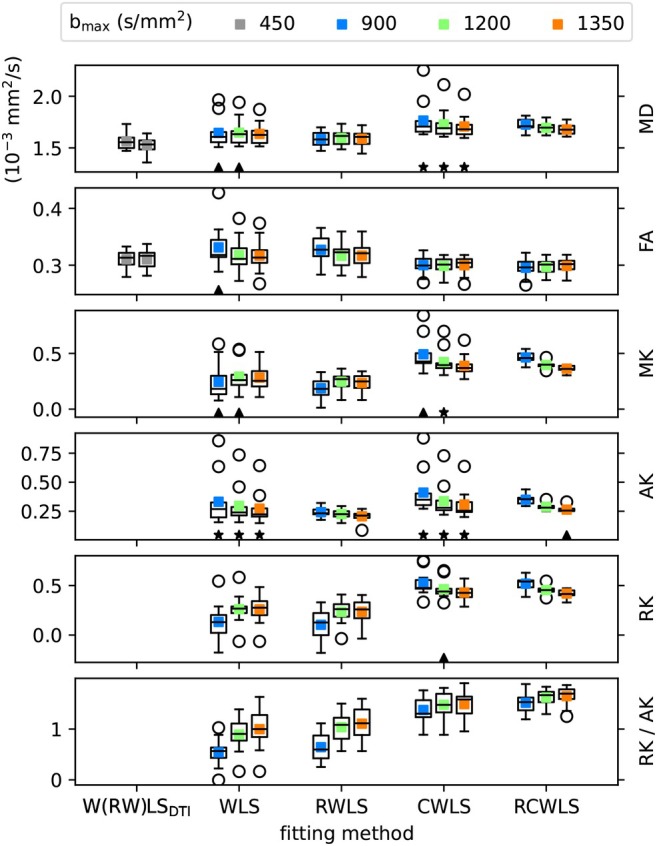 FIGURE 1
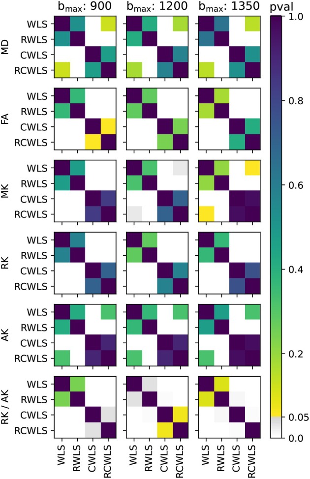 FIGURE 2
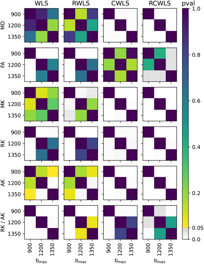 FIGURE 3
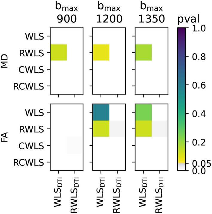 FIGURE 4
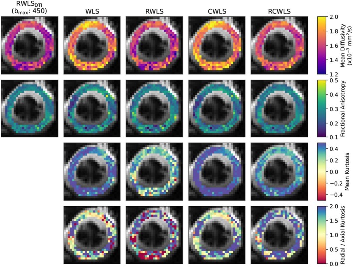 FIGURE 5
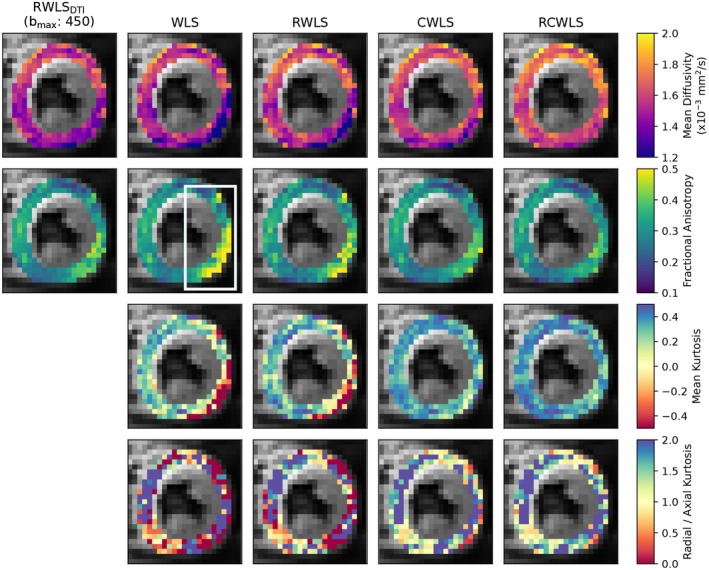 FIGURE 6
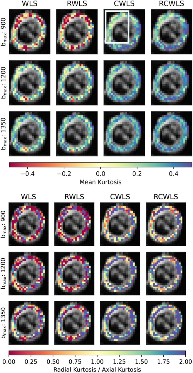 FIGURE 7
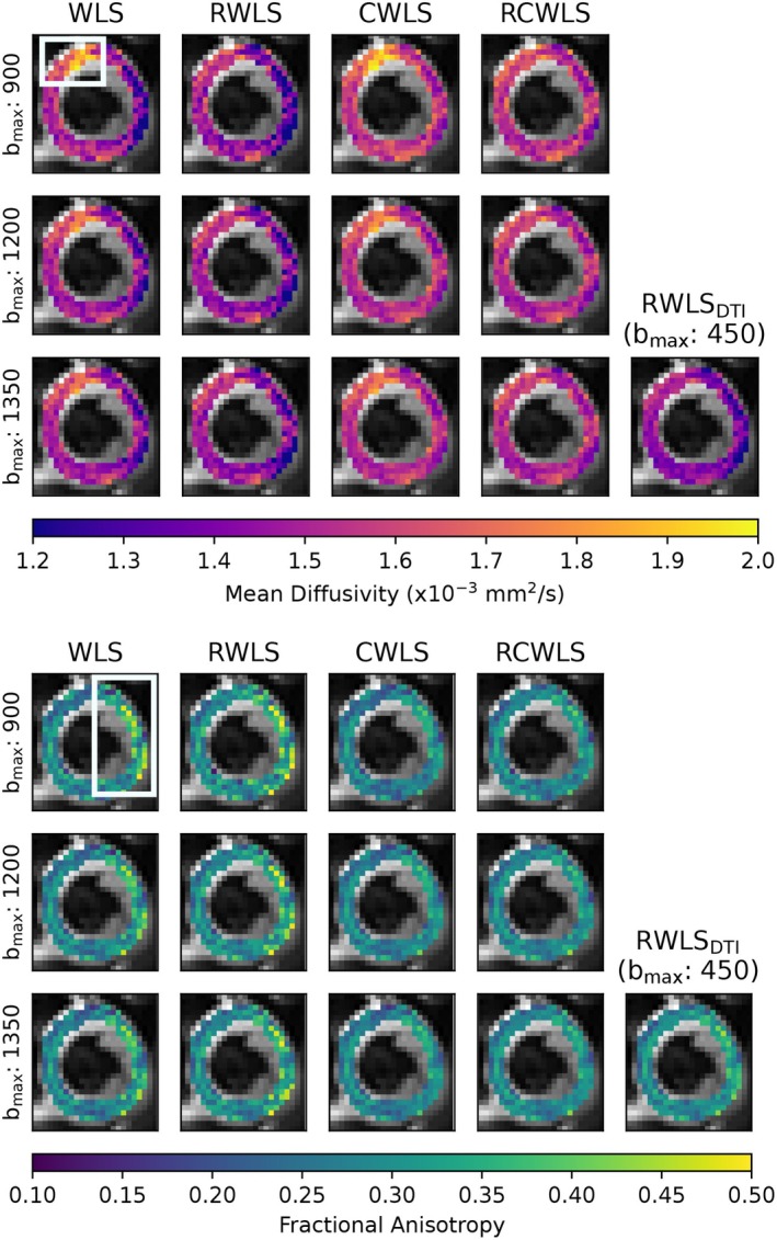 FIGURE 8
- —Wellcome Trust10.13039/100010269
Peer Reviews
No public reviews on file for this paper yet. If you reviewed it on a platform where reviews are public (OpenReview, ICLR, NeurIPS, ICML), you can paste yours below so the community can read it here.
Videos
No videos yet. Explain this paper in a talk, walkthrough, or lecture? Add one.
Taxonomy
TopicsAdvanced Neuroimaging Techniques and Applications · MRI in cancer diagnosis · Advanced MRI Techniques and Applications
INTRODUCTION
1
Cardiac diffusion weighted imaging (cDWI) is a magnetic resonance imaging (MRI) technique that can be used to investigate cardiac tissue microstructure. Cardiac diffusion tensor imaging (cDTI) is the most common cDWI method used on the heart, from which measures such as mean diffusivity (MD) and fractional anisotropy (FA) can be derived. However, the diffusion‐weighted signal in tissue deviates from monoexponential decay at higher diffusion weighting (as expressed by the b‐values) due to cell membranes and other restrictions in biological tissue.1, 2, 3 Diffusion kurtosis imaging (DKI) can quantify these deviations. Non‐Gaussian diffusion models (including DKI) have been shown to have a higher sensitivity for the detection of hypertrophy in ex vivo rat hearts compared with DTI.3 Kurtosis measures include mean kurtosis (average kurtosis across all directions), axial kurtosis (kurtosis in the primary diffusion direction) and radial kurtosis (average kurtosis in the plane perpendicular to axial kurtosis).4, 5, 6, 7, 8, 9, 10, 11, 12 Anisotropic and isotropic kurtosis can be also distinguished with q‐space trajectory imaging.13
Spin echo based DKI in the human heart in vivo is challenging due to low SNR, a short myocardial T2 (approximately 46 ms at 3.0 T14) and long echo‐times (TE), required to achieve sufficient motion compensation and b‐values. Nonetheless, acquiring data with sufficiently high b‐values for cardiac DKI has been shown to be feasible in healthy volunteers in vivo using ultra‐strong gradients (i.e. 300 mT/m) at echo times and resolutions comparable to those commonly used for conventional cDTI.15, 16, 17 However, even for the brain, which has longer T2 and significantly less motion, DKI is challenging: fitting methods need to handle data corruptions,18 but also need to yield a physically plausible signal if kurtosis measures are to be meaningful.19
Image corruption is a common problem in cDWI.20 Furthermore, motion causes additional signal variations sometimes referred to as physiological noise. In cDTI, shot rejection is usually performed in an attempt to handle corruptions where noticeably corrupted images are removed from datasets before fitting, a method that is typically time consuming and subjective. In our experience, the reduced signal at higher b‐values simultaneously causes a larger number of corruptions (including those from misregistration) and a decreased ability to perform shot‐rejection effectively. Robust estimation, in which outlier signals are identified and removed at the voxel level, is an alternative to shot rejection. Our recent work shows that robust estimation is superior to shot rejection in cDTI,21 so robust estimation in cardiac DKI is worth investigating, but has not been done yet.
Although the DKI signal representation does not correspond to a valid diffusion propagator, the fitted signal should still adhere to the physical principles governing the data‐generating process. If it does not, the fitted parameters and any measures derived from them will lack meaningful interpretation. For example, the compartment model predicts that kurtosis should be nonnegative,2, 4 and the diffusion tensor should be positive definite as in DTI. For DKI, it is not known how to enforce constraints on kurtosis via reparameterization of the fitting problem, so constraints must consider whether the predicted signal behavior is valid, for example, in,22 nonlinear optimization is (infinitely) penalized if constraints are violated. Recently, linear least squares methods have been developed for enforcing convexity constraints on the cumulant generating function, leading to correction of significant errors in brain DKI.19 These advantages should also apply to cardiac DKI.
While preventing estimated parameters from violating constraints may be seen as a form of robustness, constrained fitting itself is not inherently robust. This is because the constraints do not change the shape of the fitting cost function in parameter space, which is entirely determined by the data. As a result, outliers can still have a detrimental impact on parameter estimates. Furthermore, although robust fitting may reduce the frequency and impact of constraint violations by removing outlier signals, it cannot guarantee that the parameters that optimize the cost function will not violate the constraints. The objectives of this work are (1) to demonstrate a way of combining robust fitting21 with convexity constraints19 using iteratively reweighted least squares (IRLS) to give robust constrained weighted least squares (RCWLS) and (2) to test various fitting methods (with/without robustness and with/without constraints) on in vivo cardiac DKI data collected on a Connectom scanner to determine the effects on diffusion and kurtosis measures. To our knowledge, this is the first time that constrained estimation has been combined with robust estimation in MRI.
METHODS
2
We use the following notation: tensors are bold and uppercase; vectors are bold and lowercase; tensor and vector elements are italicized and indexed.
Diffusion kurtosis imaging
2.1
The DKI signal representation can be expressed as2:
where q=b·n1,n2,n3 is the (rescaled) wave vector (denoted this way for convenience in expressing the constraints—see Section 2.3), and i,j,k,l index physical space coordinates. The diffusion tensor D and kurtosis tensor W are both symmetric, having 6 and 15 unique elements, respectively. The signal at b=0s/mm2 is denoted by scalar quantity S0. The DTI signal representation is the same as Equation (1) but without the term containing W. Kurtosis is expressed in dimensionless form due to scaling by the mean diffusivity D‾=D11+D22+D33/3.
Expanding Equation (1) accounting for the symmetry of D and W gives the following linear expression:
The 22 coefficients in θ are related to the original parameters as follows: 6 diffusion tensor parameters θ1,…,θ6=D11,D12,D22,D13,D23,D33, 15 kurtosis tensor parameters (θ7,…,θ21)=D‾2·(W1111,W2222,W3333,W1112,W1113,W1222,W2223,W1333,W2333,W1122,W1133,W2233,W1123,W1223,W1233), and intercept θ22=−lnS0. The DTI expression would include only terms depending on θ1,…,θ6 and θ22.
Weighted least squares
2.2
Given N observations {qn,Sn|n=1…N}, the weighted least squares (WLS) estimate of the coefficients θ in Equation (2), denoted by θ^WLS, is given by:
The wavevectors qn of the nth observation can be converted to xn using Equation (2c). Given design matrix X=(x1,x2,…,xN)T, observation vector y=(lnS1,lnS2,…,lnSN)T, and weights vector w=(w1,w2,…,wN)T, a weighted design matrix and observation vector can be defined:
The WLS estimate can then be written as
For uniform weights wn=1, Equation (5) gives the ordinary least squares (OLS) estimate θ^OLS.
Convexity constraints
2.3
A useful constraint for DKI is to enforce convexity of the cumulant generating function 𝒞(q) 19:
This constraint can be enforced by using sum of squares polynomials19; the mathematical background for this can be found in.23 The semi‐definite program for solving the WLS problem subject to constraints, thus yielding the constrained WLS estimate θ^CWLS, can be written as follows:
Importantly, we have written the problem in terms of the weighted design matrix X′ and observation vector y′.
We will briefly explain Equation (7) for DKI, leaving details on the constraint matrices H(θ) and L(α) (presented here for the first time) for Appendix B. Equation (7d) defines hθ(q,s), where H𝒞(q) is the Jacobian of 𝒞(q) and the dummy variable s has the same dimensions as q. Then, hθ(q,s) is just a polynomial. Convexity of 𝒞(q) requires that hθ(q,s) is nonnegative, which can be enforced using a sum of squares polynomial representation, that is, Equation (7b) (see23). We can exactly represent hθ(q,s) using a relatively small monomial basis for e (see Appendix B). The convexity constraint is satisfied when Equation (7c) holds, that is, when H(θ)+L(α) is positive semi‐definite (PSD). Note that Equation (7) involves optimizing over coefficients θ and slack parameters α. Appendix C explains how the numerical complexity of the problem can be reduced.
Robust fitting
2.4
In DTI/DKI, WLS usually refers to solving Equation (5) by weighting the (squared) residuals of the linearized problem with the (squared) signal24:
where an initial OLS estimate θ^OLS is used to predict the signals (since the true signals are not known). Henceforth, we will use “WLS” to refer to Equation (5) using the weights in Equation (8). Correspondingly, “CWLS” will refer to constrained WLS, that is, solving Equation (7) using the weights given by Equation (8).
Importantly, neither WLS nor CWLS are intrinsically robust, and outlier data can have a detrimental effect on the estimates θ^WLS or θ^CWLS. Robust estimation can be implemented using iteratively reweighted least squares (IRLS), using weights derived from a robust estimator.18, 21, 25 Notably, for WLS in DTI/DKI, these robust weight should be chosen so as to preserve the cost function implied by Equations (3) and (8) (see21 for a derivation), such that IRLS solves the WLS/CWLS problem in a robust way. Robust fitting in the DTI/DKI literature is usually done in order to remove the influence of outlier data on the fitted signal, thus making it easier to identify outlier data so that the original problem can be solved without robust weights but also without the outliers.
A robust weighting scheme accounting for the DTI/DKI weights in Equation (8), based on the Geman–McClure M‐estimator, with K iterations, is21, 25:
where θ^∗k corresponds to the estimated coefficients for iteration k (we define unk and σ^k below). This scheme requires at least 4 iterations (in which case, a single robustly weighted fit will have been performed for k=2). As with Equation (8), the symbol ← in Equation (9) is used to mean that the quantities on the right are used to evaluate the expression for the weights on the left, for example, wn2 would be calculated using θ^∗, un, and σ^ from the first iteration. The residuals of the WLS problem are defined as the difference between the log observed signal and log predicted signal:
The noise level σ^ is estimated at the kth iteration using a robust estimator designed for the WLS problem25:
where zn≡exp(fθ(qn))un←θ^∗k, MED is the median operator and m is the number of regressors, that is, m=7 for DTI and m=22 for DKI.
Set 𝒪 contains log‐signals defined as outliers by a 3‐sigma rule, applied after the last robustly‐weighted fit:
such that the estimated coefficients θ^∗ at iteration K−2 are used to evaluate fθ(qn). If the nth log‐signal yn is defined as an outlier, then it receives a weight of zero in the last two iterations in Equation (9).
The main insight in this paper is that we can use IRLS with a robust weighting scheme designed specifically for DTI/DKI, that is, Equation (9), but we are free to choose whether to estimate the coefficients at each iteration using (unconstrained) WLS with Equation (5) or CWLS with Eqs (7). The constraints are independent of the weights, which only enter the cost function Equation (7a) through Equation (4). We will refer to IRLS with weights given by Equation (9) as robust WLS (RWLS) if Equation (5) is used at each iteration, or as robust constrained WLS (RCWLS) if Equation (7) is used at each iteration. The estimated coefficients obtained from the last iteration with weights wK are denoted as θ^RWLS for RWLS and θ^RCWLS for RCWLS. For convenience, the unconstrained OLS estimate θ^OLS is used to define weights for the first iteration for both RWLS and RCWLS. We modified DiPy26 to be able to solve RWLS and RCWLS. These modifications have been incorporated in DiPy as of v1.10.
Experimental setup and recruitment
2.5
Cardiac diffusion‐weighted images (cDWI) were acquired on a Connectom 3T research‐only MR imaging system (Siemens Healthcare, Erlangen, Germany) with a maximum gradient strength of 300 mT/m and slew rate of 200 T/m/s. An 18‐channel body receive coil was used in combination with a 32‐channel spine receive coil. Eleven healthy volunteers (with no known previous cardiac conditions) were recruited for this study: age range 20.5±1.9 years (18−24 years), weight range 64.1±11.4 kg (54−94 kg), 7 females. The study was approved by the local institutional review board (Cardiff University School of Psychology Research Ethics Committee) and all subjects provided written consent.
A prototype pulse sequence was used that enables diffusion encoding with user‐defined second‐order motion‐compensated (M0M1M2) diffusion gradient waveforms, designed with the NOW toolbox27, 28, 29, 30 (see Figure A1). The maximum gradient strength used in this study for the M0M1M2 waveform to generate the b‐value of 1350s/mm2 was 285.4 mT/m, and the maximum physiologically limited slew rate was 76.2 T/m/s.15 The cDWI parameters were TR = 3 RR‐intervals, TE = 61ms, EPI readout, field‐of‐view = 320×120mm2 using ZOnally‐magnified Oblique Multislice (ZOOM, tilted RF: excitation, tilt angle: 15°, tilted slice thickness: 20mm),29, 31 in‐plane resolution = 2.7×2.7mm2, slice thickness = 8mm, 3 short axis slices (base, mid, and apical), partial Fourier factor = 7/8, no parallel imaging, bandwidth = 2354 Hz/pixel. Each full dataset comprised of 5 b‐values (b = 100, 450, 900, 1200, 1350 s/mm2). For b≥450s/mm2, 30 directions per shell were acquired with 6 repetitions while b=100s/mm2 consisted of 3 directions with 12 repeats. Data were acquired with ECG‐gating and under free‐breathing (respiratory navigators were not employed for this work). The trigger delay was adjusted for cDWI acquisition in mid‐end systole. Saturation bands were placed around the heart. Fat suppression was performed using the SPAIR method.32 The scan time for all the diffusion weighted images was around 40 min depending on subject heart rate. Including cardiac planning, the total scan time was around one hour.
Post‐processing
2.6
Post‐processing was done using in‐house tools,20 with rigid image registration utilizing SITK33 and fitting utilizing DiPy (with our updates).26 Image registration was performed by masking a suitable b=100s/mm2 image, registering all b=100s/mm2 images to this reference image, then using the average of registered b=100s/mm2 images to register the entire dataset. Correlation was used as the registration metric, since it outperformed mutual information for high b‐value images. The DTI signal representation was then fit to b≤450s/mm2 images using RWLS, and the full image series was predicted. Each original (unmodified) image was then registered to the corresponding predicted image. This method, similar to,34 improved the registration.
After registration, we fit the DTI signal representation to the b≤450s/mm2 data using RWLS. MD, FA, and helix angle (HA) (using a cylindrical coordinate system with origin on the LV blood‐pool center) were calculated. Segmentation of the LV contours was performed with care taken to exclude voxels exhibiting strong partial‐volume effects. For regions strongly affected by artifacts, such as aliasing or susceptibility‐induced warping, fitting results do not reliably represent tissue properties. Artifact masks were defined using sectors centered on the LV blood pool, in order to ignore these parts of the myocardium when calculating voxel statistics. This masking was performed by considering the image series, as well as utilizing MD, FA, HA, root mean square error and coefficient of determination (R) from the RWLS DTI fit to b≤450s/mm2 data. Across all subjects an average of 25% of voxels were excluded. We have not utilized DKI results to identify artifacts in any way since this would likely bias comparison between the fitting methods under study.
Having registered the images and segmented the myocardium, we performed further fitting experiments on myocardial voxels only. Defining bmax as the maximum b‐value images that were utilized in a given fit (such that all images with a lower b‐value were also included), we performed the following: DTI using WLS and RWLS for bmax=450s/mm2; DKI with WLS, RWLS, CWLS, and RCWLS, for bmax values 900, 1200, and 1350s/mm2. For RWLS and RCWLS, we used K=10 iterations. We calculated the following measures in each voxel: mean diffusivity (MD), fractional anisotropy (FA), mean kurtosis (MK), axial kurtosis (AK), radial kurtosis (RK), and radial / axial kurtosis (RK/AK).2, 4 We then calculated the average of these measures over non‐artifact myocardial voxels.
Statistical methods
2.7
In order to make tractable comparisons between different fitting methods and to isolate the specific effects of constraints and robustness, we applied paired tests to measures obtained from different fitting methods for the same bmax, and different bmax for the same fitting method. Specifically, we used the Wilcoxon signed‐rank test since non‐robust methods often produced results that violate the assumption of normality (which was tested with the Shapiro‐Wilk test).
In this work, we potentially face the “multiple comparisons problem” since we compare many diffusion and kurtosis measures, for many bmax values and fitting methods. It is not obvious how to adjust significance levels in the context of comparing multiple fitting methods on the same data (particularly given that multiple different measures are calculated from the same set of estimated coefficients, and that higher bmax fits included all data with lower b‐values). Methods for adjustment of significance levels rely on independence assumptions that do not seem to apply here, especially for a comparison of fitting methods. We therefore take care to draw conclusions that are supported by the overall results.
RESULTS
3
Group analysis
3.1
Figure 1 shows boxplots of the average DTI/DKI measures for all 11 subjects. All fitting methods are shown for all bmax values. The black markers drawn along the bottom of each subplot indicate non‐normality of the data in each boxplot. Figures 2, 3, 4 show the results of significance tests between measures from the different fitting methods and different bmax shown in Figure 1. Figure 2 shows the p‐values between different methods within each bmax in order to demonstrate whether different methods make a significant difference given the same bmax. Figure 3 shows the p‐values between different bmax within each method, to see whether bmax made a significant difference in measures given the method. Additionally, Figure 4 shows p‐values between DKI methods and DTI methods for MD and FA only, grouped by bmax of the DKI fits. For b=1350s/mm2, RCWLS gave the following measures across subjects: MD 1.68±0.050×10⁻³mm2/s, FA 0.30±0.013, MK 0.36±0.027, AK 0.26±0.027, RK 0.42±0.040, and RK/AK 1.65±0.19.
Average of DTI/DKI measures over myocardial voxels for all subjects. Colored points show the average over subjects, colored by bmax. DTI fits W(RW)LSDTI show WLS (left) and RWLS (right) together for convenience. The black triangles (stars) show where the Shapiro‐Wilk test p‐value ≤0.05 (≤0.01), that is, the hypothesis of normality is rejected.
p‐values from comparing DKI measures from different fitting methods given the same bmax (units s/mm2).
p‐values from comparing DKI measures from different bmax (units s/mm2) given the same fitting methods.
p‐values from comparing MD and FA from DKI fitting methods for each bmax used for DKI fitting (units s/mm2) against DTI fitting methods (bmax=450s/mm2).
Constraints
3.1.1
(i) Adding constraints to a method, that is, going from WLS to CWLS and from RWLS to RCWLS, made a statistically significant difference on all measures, for all bmax values, as shown in Figure 2. Figure 1 shows that constraints increased all kurtosis measures MK, AK, RK, and RK/AK, the latter results showing that constraints result in increasing RK more than AK. Increased kurtosis is consistent with the constraints ensuring that fitted parameters correspond to nonnegative kurtosis. (ii) For constrained fitting, MK, RK, and AK all decrease with bmax, with Figure 3 showing these changes are significant for both CWLS and RCWLS. However, Figure 1 indicates that the ratio RK/AK appears to increase with bmax for both constrained and unconstrained fitting, although this difference is not significant between bmax=1200s/mm2 and bmax=1350s/mm2.
Robustness
3.1.2
(i) Robust fitting by itself, that is, going from WLS to RWLS, and CWLS to RCWLS, gave large changes in measures for some subjects (in particular, reducing MD and MK) but did not significantly change the mean measure values over subjects. Robust fitting generally reduces the spread of the measures over the group by correcting errors in measures for some subjects, as is visually clear in Figure 1. Non‐normality of measures was only found for non‐robust methods (with the single exception, out of such 36 tests, being AK for RCWLS at bmax=1350s/mm2). (ii) Robustness may has an effect on RK/AK; Figure 2 shows the following p‐values comparing CWLS and RCWLS: bmax=900s/mm2 (p=0.032), bmax=1200s/mm2 (p=0.068), and bmax=1350s/mm2 (p=0.024). However, in the context of multiple comparisons, where no effect of robustness was seen on other measures and a 0.05 significance threshold was not met for all bmax, this result cannot be ascribed significance.
MD and FA
3.1.3
For RWLS DTI fits, we obtained MD 1.53±0.074×10⁻³mm2/s and FA 0.31±0.017. When considering robust methods, (i) MD increases from DTI (bmax≤450s/mm2) to unconstrained DKI (see Figure 4), and from unconstrained DKI to constrained DKI (see Figure 2); FA increases from DTI to unconstrained DKI (see Figure 4) but constrained DKI results in lower FA than DTI fitting (see Figure 4). (ii) For constrained methods, as bmax increases MD decreases slightly, but there is little change in FA (see Figure 3).
Example maps
3.2
Figures 5, 6, 7, 8 show example measure maps for 4 different subjects. The colormap ranges were chosen based on the boxplots in Figure 1, in particular to emphasize whether values are above zero for MK or above one for RK/AK.
Maps for the mid slice of a single subject, for bmax=1350s/mm2. The first column shows MD and FA from DTI RWLS fitting (bmax=450s/mm2) for reference. All other columns show measures from DKI fits. In this example, robust fitting decreases MK, while constrained fitting increases MK. Using robust and constrained fitting (RCWLS) gives the most plausible results, with mostly RK/AK > 1 values.
Measure maps for the mid slice of a single subject, for bmax=1350s/mm2. The first column shows MD and FA from DTI RWLS fitting (bmax=450s/mm2) for reference. All other columns show measures from DKI fits. Around 2 to 6 o'clock for the DKI fits is a region of implausibly low MD, high FA, and negative MK, for unconstrained fits. Constraints correct this region towards plausible values, with robust fitting visibly improving the region further in the same direction.
Mean kurtosis (MK) and radial kurtosis / axial kurtosis (RK/AK) maps for the basal slice of a single subject, for all bmax values (units s/mm2) used for DKI fitting methods. Constraints increase MK given the same bmax. For constrained fitting (CWLS and RCWLS), MK decreases with bmax in most voxels but increases between 8 and 12 o'clock. RCWLS for bmax=1350s/mm2 has the most spatially homogeneous MK.
Mean diffusivity (MD) and fractional anisotropy (FA) maps for the basal slice of a single subject, for all bmax values (units s/mm2) used for DKI fitting methods. Also shown are MD and FA from RWLS DTI fitting (bmax=450s/mm2) for reference. Robust fitting corrects elevated MD in the top‐left (10–12 o'clock), but constraints are needed to correct the reduced MD and elevated FA on the right (12–5 o'clock).
Figure 5 shows basal‐slice maps for bmax=1350s/mm2 for the subject with the second highest MD and MK for non‐robust fitting WLS/CWLS in Figure 1. Robust fitting gave large changes over the whole myocardium, bringing measures into better agreement with other subjects, such that for robust fitting methods this subject is no longer an outlier in the boxplots of Figure 1. MD and MK are reduced, and FA is increased, for robust methods vs non‐robust methods. Constraints increase MK and RK/AK, which is most noticeable between RWLS and RCWLS. In particular for RCWLS, RK/AK > 1 in nearly every voxel and is relatively homogeneous. This example shows that kurtosis can appear to be positive for non‐constrained methods, but these kurtosis measures can still be corrupted. Going from WLS to RWLS results in a large reduction of MK, indicating that its consistently positive value for WLS was likely due to corruptions in the data (which, in this case, also caused an inflation of MD). By adding constraints to robust fitting, that is, going from RWLS to RCWLS, consistently positive MK is recovered, but with much lower values than from the WLS fit.
Figure 6 shows mid‐slice maps for bmax=1350s/mm2 where robust fitting had large effects in a localized region (around 2 to 6 o'clock) with low MD, high FA, and negative MK for WLS. Here, both robust fitting and constraints independently increase MD, reduce FA, and increase MK, such that RCWLS gives the most spatially uniform values. The regions where RK/AK is around 1 for RCWLS coincide with relatively lower FA.
Figure 7 shows MK and RK/AK basal‐slice maps for different bmax. Constraints give positive MK and make RK/AK > 1 overall. Reading across the rows, constraints increase MK and RK / AK given the same bmax. Differences between unconstrained and constrained fitting decrease with bmax. Reading down the RCWLS column, MK decreases with bmax for most voxels but increases between 8 and 12 o'clock. These opposing effects result in RCWLS for bmax=1350s/mm2 having the most homogeneous MK.
Figure 8 shows MD and FA maps in a basal slice for different bmax and for DTI fitting (bmax=450s/mm2). Robust fitting corrects elevated MD in the top‐left (10–12 o'clock), but constraints are needed to correct the reduced MD and elevated FA on the right (12–5 o'clock). The effects on MD and FA are consistent with the overall group trends. RCWLS gives the most homogeneous MD and FA, with the least variation with bmax.
DISCUSSION
4
Our results show that both robust fitting and convexity constraints affect DTI/DKI measures in important ways. Figure 5 helps to show that the RCWLS results are not just the robust result with the negative kurtosis turned to zero—the kurtosis becomes convincingly positive, and all measures change when adding constraints. In this case, robust fitting reduced inflated MK caused by corruptions, while adding constraints increased MK. Figure 6 demonstrates a region where only robust fitting and constraints together appear to fully resolve a region of corrupted measures. In theory, RCWLS provides advantages greater than the sum of its parts: convexity constraints should make outlier identification easier, which should improve the weights in the final WLS fit.
Constraints
4.1
Imposing convexity constraints resulted in statistically significant differences in all measures for all bmax values. The precise changes, notably increased MK and RK/AK, are important. Only constrained fitting reliably shows RK > AK (for RCWLS bmax=1350s/mm2, RK/AK mean and median are 1.65 and 1.70 respectively), despite this being expected in myocardium since there are fewer restrictions to diffusion parallel to the long axes of cardiomyocytes.3, 35 It is worth emphasizing that adding constraints does not just turn negative kurtosis into zero kurtosis in certain voxels (something that could be trivially obtained in post‐processing the fitting results), but fundamentally alters the optimum coefficient vector (Figures 5 and 6).
Robustness
4.2
Robust fitting can have large overall and regional benefits on individual subjects, which is invaluable for potential clinical applications. Variation between subjects within a group ought to represent physiological variation (and non‐gross measurement error) rather than the effects of image corruptions. In the context of a study comparing different groups (e.g., healthy volunteers vs. disease), the reduction in the spread of measures from robust fitting can increase statistical power and lower the probability of a type 2 errors (false negatives).21
MD and FA
4.3
While it is known that MD and FA obtained from fitting the DKI signal representation can be different compared to those obtained from the DTI signal representation,36 constraints further modify these values: MD increases from DTI to DKI and from unconstrained to constrained fitting, but while FA increases from DTI to DKI, it decreases from unconstrained to constrained fitting, resulting in RCWLS giving the lowest FA values. This shows that the FA changes from DTI to DKI were largely in the context of parameter fits that violated constraints. To the best of our knowledge, other works noting differences in MD and FA between DTI and DKI have not utilized constraints or robust fitting.
bmax effect
4.4
Varying bmax allowed for investigating the importance of constraints and robustness for different experimental designs: higher bmax data is more informative about kurtosis but has lower SNR. While previous work has noted the dependence of the performance of (simplified models of) cardiac DKI on bmax,3 it is noteworthy that MK and RK appear to increase with bmax for unconstrained fitting, but decrease with bmax for constrained fitting. This only serves to emphasize the importance of using fitting constraints. Due to these opposite trends, the differences between unconstrained and constrained fitting get smaller as bmax increases, suggesting fewer and milder constraint violations as data become more informative about kurtosis.
Limitations
4.5
Although the differences between non‐robust and robust methods were generally insignificant at the group level, the errors from non‐robust methods would make the detection of any actually existing differences quite challenging, which is perhaps ironic. It is also true that summary statistics such as mean measures over all voxels can be insensitive to the improvement in measure maps when using robust fitting, and yet post hoc statistical analysis of regions of interest (where measures were most changed by robust methods) would also seem problematic. The only measure that indicated any potential effect (at the group level) from robust fitting alone was RK/AK, particularly for bmax=1350s/mm2 (p = 0.024), but we cannot rule out a false positive here due to multiple comparisons of many measures. The ratio RK/AK might be more sensitive to changes from robust fitting, but more subjects would be required to have sufficient statistical power to determine this.
Higher bmax fits included all lower b‐values, and so there is more data available for these fits. Our study sought to determine how the results changed as more information about kurtosis was available, specifically in the context of understanding the effects of robust fitting and constrained fitting, so the conflation from having both higher b‐value data (which has lower SNR) and more data overall was not of particular concern. To perform an analysis about the suitability of different data designs, we believe many more subjects would be required, as well as a more nuanced analysis of trends with bmax (rather than just paired tests). This work could be restricted to robust and constrained fitting methods.
A limitation of signal representations, such as DTI and DKI, is a lack of clear insight into the specific quantitative links to the underlying biology: differences in kurtosis measures between groups can be observed and reasoned about, but the absolute values are not ascribed any particular meaning.3 Nonetheless, we can speculate that kurtosis measures (derived from appropriate fitting techniques) may be a way to increase the biomarker space and gain insight into disease; further work is required.
CONCLUSION
5
In this work, we have developed robust constrained weighted least squares (RCWLS), the first robust estimation technique for DKI that incorporates necessary constraints on the signal behavior. Using in vivo human cardiac DKI data from healthy volunteers collected with a Connectom scanner, we determined that RCWLS is the most suitable fitting technique compared with others that lack either robustness or constraints. For b=1350s/mm2, RCWLS gave the following measures across subjects: MD 1.68±0.050×10⁻³mm2/s, FA 0.30±0.013, MK 0.36±0.027, AK 0.26±0.027, RK 0.42±0.040, and RK/AK 1.65±0.19. Constraints, but not robustness, had a significant effect on all diffusion and kurtosis measures. However, robust fitting corrected large errors for some subjects and generally improved diffusion and kurtosis maps. Only RCWLS convincingly showed radial kurtosis to be larger than axial kurtosis for all subjects, something that is expected in myocardium due to increased restrictions to diffusion in the plane perpendicular to the primary myocyte direction. RCWLS also showed the best correction of corrupted regions in diffusion parameter maps for individual subjects. Future work on in vivo cardiac DKI should utilize fitting techniques that are both robust and constrained, such as RCWLS.
CONFLICT OF INTEREST
The authors declare no potential conflict of interests.
The reference list from the paper itself. Each links out to its DOI / PubMed record.
- 1Alexander DC , Barker GJ , Arridge SR . Detection and modeling of non‐Gaussian apparent diffusion coefficient profiles in human brain data. Magn Reson Med. 2002;48:331‐340.12210942 10.1002/mrm.10209 · doi ↗ · pubmed ↗
- 2Jensen JH , Helpern JA , Ramani A , Lu H , Kaczynski K . Diffusional kurtosis imaging: the quantification of non‐gaussian water diffusion by means of magnetic resonance imaging. Magn Reson Med. 2005;53:1432‐1440.15906300 10.1002/mrm.20508 · doi ↗ · pubmed ↗
- 3Mc Clymont D , Teh I , Carruth E , et al. Evaluation of non‐Gaussian diffusion in cardiac MRI. Magn Reson Med. 2017;78:1174‐1186.27670633 10.1002/mrm.26466 PMC 5366286 · doi ↗ · pubmed ↗
- 4Jensen JH , Helpern JA . MRI quantification of non‐Gaussian water diffusion by kurtosis analysis. NMR Biomed. 2010;23:698‐710.20632416 10.1002/nbm.1518 PMC 2997680 · doi ↗ · pubmed ↗
- 5Tabesh Ali A , Jensen JH , Ardekani BA , Helpern JA . Estimation of tensors and tensor‐derived measures in diffusional kurtosis imaging. Magn Reson Med. 2011;65:823‐836.21337412 10.1002/mrm.22655 PMC 3042509 · doi ↗ · pubmed ↗
- 6Basser PJ , Pierpaoli C . Microstructural and physiological features of tissues elucidated by quantitative‐diffusion‐tensor MRI. J Magn Reson. 2011;213:560‐570.22152371 10.1016/j.jmr.2011.09.022 · doi ↗ · pubmed ↗
- 7Russell GG , Helpern JA , Tabesh A , Jensen JH . Quantitative assessment of diffusional kurtosis anisotropy. NMR Biomed. 2015;28:448‐459.25728763 10.1002/nbm.3271 PMC 4378654 · doi ↗ · pubmed ↗
- 8Hansen B , Shemesh N , Jespersen SN . Fast imaging of mean, axial and radial diffusion kurtosis. Neuroimage. 2016;142:381‐393.27539807 10.1016/j.neuroimage.2016.08.022PMC 5159238 · doi ↗ · pubmed ↗