Great Wall: A Generalized Dose Optimization Design for Drug Combination Trials Maximizing Survival Benefit
Yan Han, Yingjie Qiu, Yi Zhao, Isabella Wan, Lang Li, Suyu Liu, Yong Zang

TL;DR
The Great Wall design is a new method for drug combination trials that aims to maximize long-term survival benefits by optimizing dose combinations based on toxicity and early efficacy.
Contribution
The Great Wall design introduces a modular dose optimization approach that addresses partial order toxicity and balances early efficacy with long-term survival outcomes.
Findings
The Great Wall design uses a divide-and-conquer algorithm to handle partial order toxicity and eliminate suboptimal dose combinations.
Simulation studies show the design has desirable operating characteristics across various clinical settings.
The design is modular and practical for trials where long-term survival outcomes are assessed.
Abstract
Most phase I–II drug‐combination trial designs assume that selecting the optimal dose combination based on early outcomes will also lead to maximum long‐term survival benefits. However, this assumption is often violated in many clinical studies, generally due to high rates of relapse following the initial response. To address this problem, we propose the Great Wall design, a general dose optimization design for drug‐combination trials. The Great Wall design employs a “divide‐and‐conquer” algorithm to address the issue of partial order of toxicity and uses early outcomes to eliminate dose combinations that are excessively toxic or less efficacious. It utilizes a dose randomization approach to construct a candidate set of the promising dose combinations balancing the toxicity and early efficacy outcomes. The patients assigned to the candidate set are followed to collect the survival…
Genes, proteins, chemicals, diseases, species, mutations and cell lines named across the full text — each resolved to its canonical identifier and authoritative record.
Click any figure to enlarge with its caption.
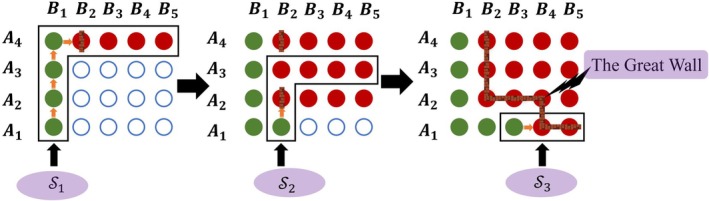 FIGURE 1
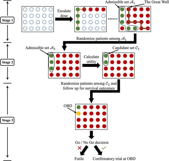 FIGURE 2
| Drug B | Drug B | |||||
|---|---|---|---|---|---|---|
| 1 | 2 | 3 | 1 | 2 | 3 | |
| Drug A | Scenario 1 | Scenario 2 | ||||
| 2 | (0.60,0.20, 0.28,0.25) | (0.67,0.40, 0.37,0.50) | (0.75,0.30, 0.28,0.40) | (0.25,0.45, 0.57,0.10) | (0.40,0.55, 0.57,0.15) | (0.50,0.50, 0.50,0.20) |
| 1 | (0.5,0.10, 0.26,0.20) | (0.62,0.20, 0.27,0.40) | (0.68,0.30, 0.31,0.50) | (0.10,0.40, 0.60,0.05) | (0.35,0.50, 0.56,0.10) | (0.45,0.50, 0.52,0.25) |
| Drug A | Scenario 3 | Scenario 4 | ||||
| 2 | (0.20,0.53, 0.64,0.35) | (0.40,0.40, 0.48,0.25) | (0.50,0.40, 0.44,0.40) | (0.10,0.3, 0.54,0.35) |
| (0.45,0.55, 0.55,0.40) |
| 1 |
| (0.35,0.60, 0.62,0.35) | (0.45,0.60, 0.58,0.20) | (0.05,0.20, 0.50,0.20) | (0.10,0.40, 0.60,0.40) | (0.40,0.40, 0.48,0.45) |
| Drug A | Scenario 5 | Scenario 6 | ||||
| 2 |
| (0.20,0.60, 0.68,0.25) | (0.45,0.45, 0.49,0.35) | (0.10,0.60, 0.72,0.42) | (0.25,0.60, 0.66,0.42) | (0.48,0.65, 0.60,0.30) |
| 1 | (0.10,0.20, 0.48,0.20) | (0.15,0.30, 0.52,0.25) | (0.40,0.30, 0.42,0.40) | (0.08,0.30, 0.55,0.25) |
| (0.42,0.55, 0.56,0.35) |
| Drug A | Scenario 7 | Scenario 8 | ||||
| 2 | (0.12,0.20, 0.47,0.20) | (0.15,0.58, 0.69,0.40) | (0.17,0.62, 0.70,0.40) | (0.06,0.20, 0.50,0.25) | (0.10,0.40, 0.60,0.40) |
|
| 1 | (0.08,0.14, 0.45,0.20) | (0.12,0.30, 0.53,0.25) |
| (0.02,0.10, 0.45,0.20) | (0.05,0.20, 0.50,0.35) |
|
| Designs | Sel % | No Sel % | Pat % | Sample size | ||||
|---|---|---|---|---|---|---|---|---|
| Scenario 1 | ||||||||
| Great Wall | 0.0 | 0.0 | 0.0 |
| 14.3 | 3.2 | 0.5 | 32.2 |
| 0.6 | 0.0 | 0.0 | 65.3 | 13.7 | 3.0 | |||
| CONV1 | 0.0 | 0.0 | 0.0 |
| 15.6 | 3.6 | 0.6 | 39.2 |
| 11.1 | 0.0 | 0.0 | 63.6 | 13.9 | 3.0 | |||
| CONV2 | 2.1 | 0.1 | 0.0 |
| 11.1 | 0.4 | 0.0 | 33.2 |
| 1.1 | 0.4 | 0.0 | 87.1 | 1.3 | 0.0 | |||
| Scenario 2 | ||||||||
| Great Wall | 0.2 | 0.3 | 0.0 |
| 23.5 | 10.9 | 5.1 | 72.0 |
| 0.0 | 0.3 | 1.2 | 32.6 | 19.3 | 8.6 | |||
| CONV1 | 21.2 | 4.1 | 0.2 |
| 22.4 | 13.4 | 6.6 | 72.0 |
| 48.3 | 19.5 | 3.9 | 29.0 | 18.5 | 10.1 | |||
| CONV2 | 0.0 | 0.1 | 7.4 |
| 28.2 | 14.8 | 3.8 | 73.5 |
| 0.1 | 0.4 | 0.1 | 18.5 | 22.7 | 12.1 | |||
| Scenario 3 | ||||||||
| Great Wall | 5.6 | 0.1 | 0.0 | 3.1 | 25.1 | 11.2 | 5.3 | 71.7 |
|
| 4.9 | 0.0 | 31.3 | 18.7 | 8.4 | |||
| CONV1 | 18.3 | 0.2 | 0.0 | 3.0 | 23.9 | 13.9 | 6.6 | 72.0 |
|
| 15.2 | 2.4 | 28.7 | 17.6 | 9.3 | |||
| CONV2 | 19.7 | 7.4 | 4.8 | 18.3 | 26.2 | 17.8 | 4.9 | 73.6 |
|
| 26.8 | 1.6 | 17.1 | 21.4 | 12.7 | |||
| Scenario 4 | ||||||||
| Great Wall | 5.3 |
| 0.3 | 1.9 | 19.3 | 21.6 | 8.9 | 73.1 |
| 0.3 | 11.1 | 4.0 | 18.0 | 20.6 | 11.6 | |||
| CONV1 | 5.9 |
| 1.7 | 0.9 | 19.9 | 17.8 | 10.7 | 73.0 |
| 2.8 | 21.7 | 3.1 | 19.8 | 19.0 | 12.8 | |||
| CONV2 | 2.5 |
| 26.7 | 2.9 | 8.7 | 26.8 | 24.0 | 73.9 |
| 0.0 | 3.0 | 6.4 | 5.8 | 12.3 | 22.5 | |||
| Scenario 5 | ||||||||
| Great Wall |
| 8.6 | 0.8 | 19.1 | 21.9 | 20.2 | 8.2 | 71.2 |
| 1.7 | 6.3 | 6.0 | 19.5 | 19.3 | 11.0 | |||
| CONV1 |
| 55.4 | 0.9 | 2.7 | 19.9 | 16.8 | 9.9 | 72.1 |
| 5.2 | 11.9 | 1.8 | 21.1 | 19.3 | 13.0 | |||
| CONV2 |
| 8.0 | 16.1 | 25.6 | 12.8 | 23.8 | 17.6 | 73.6 |
| 0.0 | 6.1 | 28.7 | 10.0 | 15.1 | 20.7 | |||
| Scenario 6 | ||||||||
| Great Wall | 20.4 | 8.9 | 0.1 | 2.5 | 24.1 | 17.0 | 7.6 | 71.8 |
| 1.2 |
| 1.2 | 19.6 | 20.7 | 11.0 | |||
| CONV1 | 52.6 | 15.3 | 0.8 | 1.9 | 21.2 | 17.0 | 9.4 | 72.7 |
| 2.4 |
| 3.8 | 21.4 | 19.0 | 12.0 | |||
| CONV2 | 6.5 | 26.0 | 8.3 | 10.1 | 12.3 | 28.1 | 14.0 | 73.8 |
| 0.7 |
| 12.5 | 7.9 | 16.8 | 20.8 | |||
| Scenario 7 | ||||||||
| Great Wall | 0.3 | 11.2 | 8.4 | 3.8 | 14.3 | 18.7 | 16.7 | 72.1 |
| 0.1 | 0.7 |
| 14.6 | 16.1 | 19.5 | |||
| CONV1 | 0.3 | 27.1 | 28.9 | 1.6 | 18.0 | 16.6 | 14.2 | 72.6 |
| 0.3 | 2.7 |
| 18.1 | 17.1 | 16.0 | |||
| CONV2 | 0.3 | 1.6 | 60.3 | 7.9 | 9.9 | 12.6 | 47.4 | 73.8 |
| 0.0 | 0.8 |
| 7.1 | 2.2 | 20.8 | |||
| Scenario 8 | ||||||||
| Great Wall | 0.3 | 4.2 |
| 0.5 | 15.0 | 18.2 | 22.7 | 73.8 |
| 0.0 | 1.3 |
| 13.7 | 15.0 | 15.5 | |||
| CONV1 | 1.3 | 8.2 |
| 0.1 | 17.8 | 17.2 | 15.2 | 73.9 |
| 0.2 | 1.7 |
| 16.8 | 16.7 | 16.2 | |||
| CONV2 | 0.0 | 6.7 |
| 0.1 | 5.6 | 9.6 | 63.8 | 73.9 |
| 0.0 | 0.0 |
| 4.4 | 0.3 | 16.3 | |||
- —National Cancer Institute10.13039/100000054
- —National Institute of General Medical Sciences10.13039/100000057
- —Ralph W. and Grace M. Showalter Research Trust Fund10.13039/100007114
- —Indiana CTSI10.13039/100006975
Peer Reviews
No public reviews on file for this paper yet. If you reviewed it on a platform where reviews are public (OpenReview, ICLR, NeurIPS, ICML), you can paste yours below so the community can read it here.
Videos
No videos yet. Explain this paper in a talk, walkthrough, or lecture? Add one.
Taxonomy
TopicsStatistical Methods in Clinical Trials · Optimal Experimental Design Methods · Advanced Causal Inference Techniques
Introduction
1
The drug combination strategy, which involves administering two or more drugs together, has become popular due to its enhanced effectiveness and ability to delay drug resistance [1, 2, 3]. A notable example is the HER2‐positive breast cancer trial [4], where combining trastuzumab with chemotherapy significantly increased survival rates compared to chemotherapy alone.
A unique feature of the drug combination trials is that the toxicity order among dose combinations is only partially clear due to unknown drug–drug interaction effects, making the drug combination trial design more challenging than the single‐agent trial design [5]. Still, many phase I dose‐finding designs for drug combination trials have been proposed, which aim to identify the maximum tolerated dose (MTD) or MTD contour (e.g., multiple MTDs) based on the toxicity outcomes [6, 7, 8, 9, 10, 11, 12, 13].
Molecularly targeted agents (MTAs) and immunotherapies (ITs) have revolutionized cancer treatment. Unlike cytotoxic agents, the principle of “more is better” does not always apply to MTAs and ITs. Increasing their dose beyond the optimal therapeutic range may not enhance outcomes and could increase toxicity. Therefore, phase I–II trials for these agents focus on identifying the optimal biological dose (OBD), which balances toxicity and efficacy [14, 15]. Various dose optimization designs exist for drug combination trials to determine the OBD combination (ODC) [16, 17, 18, 19, 20, 21, 22, 23, 24].
In most phase I–II trials, early efficacy endpoints, like objective tumor response rate, are used to determine the OBD, followed by a phase III trial to confirm survival benefit. This approach aims to expedite dose optimization but has some very undesirable drawbacks. Firstly, small early‐phase sample sizes can lead to an OBD that proves unsafe or ineffective in sequential trials. Moreover, if short‐term efficacy is not a good surrogate for survival, there is a high risk of selecting a suboptimal dose for survival outcomes [25].
Identifying the OBD based solely on early outcomes without considering survival carries risks, as shown by a phase II trial comparing busulfan plus melphalan (B+M) with melphalan (M) alone for multiple myeloma. The trial was terminated early due to lower response rates for B+M (13.6%) versus M (40.6%). However, post hoc analysis revealed 12‐month PFS probabilities of 0.90 for B+M versus 0.77 for M, leading to a redesign with PFS as the primary outcome [26]. This highlights that early efficacy may not always correlate with survival. Recent hybrid designs [27, 28, 29] integrate early and long‐term outcomes, but none are tailored for drug–drug combination trials.
In 2021, FDA initiated Project Optimus [30] which aims to improve oncology drug development by shifting focus from the traditional maximum tolerated dose (MTD) based approach to more evidence‐based dosing strategies. A key component of this initiative is the emphasis on dose randomization during clinical trials. Rather than testing only the highest tolerated dose, dose randomization involves evaluating multiple dose levels across trial participants. This allows for a more comprehensive understanding of the drug's efficacy and safety profile at different doses and higher accuracy in identifying the true optimal dose.
In this paper, we propose the Great Wall design, a new dose optimization design for drug–drug combination trials that integrates dose escalation and adaptive dose randomization to identify the ODC maximizing survival benefit. The design consists of three stages. In stage 1, a “divide‐and‐conquer” dose escalation algorithm rapidly explores the toxicity and early efficacy profiles, establishing a set of admissible dose combinations based on early outcomes. Stage 2 randomizes more patients to the admissible set and refines it using a mean utility criterion that balances toxicity and efficacy to construct the candidate set. In stage 3, patients are further randomized to the candidate set, with survival outcomes used to select the final ODC at the end of the trial.
Adaptive Design
2
Consider a drug combination trial with two drugs, A and B, each with multiple doses, A1<⋯<AJ, and B1<⋯<BK, respectively. Without loss of generality, the doses of drug A are arranged in descending order vertically, while the doses of drug B are arranged in ascending order horizontally. The dose combinations are represented in a J×K matrix, where the optimal dose combination (ODC) maximizes survival benefit while maintaining acceptable toxicity. We propose the Great Wall design, a three‐stage approach that identifies the ODC by evaluating toxicity (e.g., DLT), early efficacy (e.g., tumor response), and survival outcomes.
Stage 1 involves a rapid toxicity assessment to eliminate dose combinations with unacceptable toxicity. However, the toxicities are monotonically increasing among the dosage of one drug only if the dosage for the other drug is fixed, known as the partial toxicity order. To address this issue, we employ a “divide and conquer” algorithm that divides the dose matrix into sub‐paths, ensuring ordered toxicity probabilities within each, allowing for the use of single‐agent dose‐finding methods.
Starting with the original dose matrix M1, the first sub‐path S1 includes the dose combinations in the leftmost column and top row, arranged in increasing toxicity as:
Unlike the conventional dose‐finding designs identifying MTD, dose escalation following this sequence aims to identify combinations with excessive toxicity, without the need to retain doses. Therefore, the dose escalation process continues as long as the current dose remains safe.
Let ld represent the number of patients treated at current dose combination d, and xT,d be the number who experienced DLTs. The toxicity probability estimate is p^T,d=xT,dld, and ψ denotes the threshold for excessive toxicity. If p^T,d<ψ, we continue dose escalation within S1. If p^T,d≥ψ, escalation stops, and the current dose combination and all the combinations beyond are deemed overly toxic.
We propose a model‐assisted design framework to optimize ψ. Let ∅T be the well‐tolerated toxicity probability, and ρ∅T be the toxicity rate that is deemed overly toxic (e.g., ρ=1.4 following the BOIN design). We formulate two simple hypotheses at current dose combination as:
So, if H0 is true, the correct decision is to keep the dose escalation, which would happen only if p^T,d<ψ is observed. Similarly, if H1 is true, the correct decision is to terminate the dose escalation with p^T,d≥ψ being observed. Finally, the overall correct decision probability is:
where
Let bd=floorldψ−1 and assign equal priors PrH0 and PrH1, Pψ can be expressed as
Because ρ>1, ∅Tρ∅TxT,d1−∅T1−ρ∅Tld−xT,d monotonically decreasing with xT,d. Therefore, given 12ldxT,dρ∅TxT,d1−ρ∅Tld−xT,d>0, Pψ is maximized when
This leads to optimal value of ψ:
A key feature of the “divide and conquer” algorithm is its ability to reduce the searching space for subsequent sub‐paths automatically. For instance, if during dose escalation in sub‐path S1, the dose combination AjBk is deemed overly toxic, then any combination AjBk with j*>j or k*>k is also overly toxic and excluded. Let E1 be these excluded combinations. After S1, the search space reduces to M2=M1\S1∪E1, and this process is repeated for all sub‐paths.
We acknowledge that there are multiple ways to configure sub‐paths, and the configuration used in this paper is for illustration only. In practice, physicians can tailor configurations based on clinical and pharmacometric knowledge of toxicity profiles. For example, if increasing drug B's dosage potentially induces more overlapping toxicity than drug A, sub‐paths can prioritize escalating drug A to enhance safety. Nevertheless, the proposed dose escalation design is flexible and applicable to any reasonable configuration.
Figure 1 illustrates stage 1 of the Great Wall design in a 4 × 5 drug combination trial. Green represents safe doses, red denotes unsafe ones, and hollow circles indicate untried doses. The first sub‐path is S1=A1B1A2B1A3B1A4B1A4B2A4B3A4B4A4B5. We start at A1B1 and escalate through S1 until A4B2 is identified as overly toxic and build the first “wall” there. The searching space reduces to M2=M1\S1 and S2=A1B2A2B2A3B2A3B3A3B4A3B5. By escalating through S2 we identify A2B2 as overly toxic, forming the second wall and further reducing space. The final search space is S3=A1B3A1B4A1B5. After building the third wall at A1B4, “the Great Wall” can be constituted by linking all the walls together. Then, all the doses below the “the Great Wall” are safe and can be moved to the next stage.
An illustrative example for stage 1 of the Great Wall design.
Stage 1 primarily focuses on toxicity outcomes for dose escalation, but early efficacy and survival outcomes can also be collected if the trial's eligibility criteria remain consistent across stages. This seamless data integration enhances the identification of the ODC. However, if no major efficacy benefit is expected for patients enrolled in stage 1, only toxicity outcomes should be collected. For this paper, we assume population homogeneity and collect all outcomes starting from stage 1.
Let AT,1 be the admissible set of toxicity for stage 1, including all the dose combinations below the Great Wall. This set is further refined by eliminating dose combinations with ineffective early efficacy profiles. For each d∈AT,1, we assign a Beta prior distribution Beta1,1 for the early efficacy probability pE,d. Based on the observed data D1 in stage 1, we can derive the corresponding posterior distribution pE,dD1, also from a Beta distribution. Then, let ∅E be the fixed lower limit for the early efficacy endpoint, the admissible set for stage 1, including dose combinations with acceptable toxicity and early efficacy profiles, is:
We use 0.05 as the cut‐off for unacceptable early efficacy, with 0.05 to 0.2 generally working well in preliminary simulations. Due to the limited sample size used in stage 1, the purpose of developing A1 is to exclude the dose combination that are extremely toxic or inefficacious rather than providing a comprehensive toxicity and efficacy evaluation. A small cut‐off value provides such flexibility and has been widely adopted in various dose optimization designs [14, 27, 28, 29]. The value can also be determined by clinicians to reflect different clinical requirements.
In stage 1, the inability to retain doses limits us to assigning only one cohort per dose combination, impacting the accuracy of our estimates. In stage 2, we equally randomize additional n2 patients among the admissible set A1 and gather data D2. Although toxicity profiles were assessed in stage 1, the primary objective is to exclude overly toxic dose combinations rather than to pinpoint the MTD contours. In clinical practice, it is generally infeasible to select an ODC beyond the MTD contour. Therefore, by the end of stage 2, we aim to enhance trial safety by identifying the MTD contour.
We begin by estimating toxicity probabilities for all the tested dose combinations based on the combined data D1∪D2, using matrix isotonic regression [10] to preserve partial toxic ordering. Then, for each row of the dose matrix, we select the MTD as the dose combination with a toxicity estimate closest to the well‐tolerated toxicity rate ∅T, provided no combination is excessively toxic. The dose combinations at or below the MTD contour constitute the stage 2 toxicity admissible set AT,2. After updating the posterior distribution pE,dD1∪D2, the stage 2 overall admissible set is:
Since A2 may include many dose combinations, we streamline it by selecting the most promising candidates using the mean utility function, which balances toxicity and early efficacy.
Let YT represent the binary toxicity outcome (YT=1 for DLT, YT=0 otherwise) and YE represent early efficacy (YE=1 for complete or partial remission, YE=0 otherwise). We define πa,bd=PrYE=aYT=bd as the joint probability for YEYT at dose combination d, where a,b∈0,1. To establish utility, we assign U1,0=100 to the most desirable outcome YE=1YT=0, and U0,1=0 to the least desirable YE=0YT=1. Clinicians can then provide subjective utility scores for YE=1YT=1 and YE=0YT=0 between 0 and 100.
The mean utility of dose d, normalized between 0 and 1, is U¯d=1100∑a=01∑b=01Ua,bπa,bd.
This approach can handle ordinal endpoints and is easily interpretable for clinicians, making it widely used in early‐phase trial designs [14].
Let ld be the number of patients treated at the dose combination d and xa,b,d of them have experienced the event YE=aYT=b. At the end of stage 2, for each dose combination d∈A2, by plugging in the simple proportional estimates πa,b^d=xa,b,dld, we calculate U^dD1∪D2 as the estimate of the mean utility at dose combination d using the accumulated data D1∪D2, and identify U^max=maxU^dD1∪D2d∈A2. Then, we can construct the candidate dose set for stage 2 as:
γ in (4) determines the flexibility of candidate set selection. For example, if γ=70%, then any dose combination d∈A2 with estimated mean utility at least 70% of the maximum value is included in the candidate set.
In stage 3, after establishing C2, we randomize the final cohort of n3 patients equally within C2. We then complete follow‐ups for all patients assigned to C2 throughout the trial, collecting survival and toxicity data. Using the cumulative toxicity data, we construct the final MTD contour and update the candidate dose set to C3, excluding doses above the contour to further strengthen the safety. Let ψSd represent the dose‐optimality criterion (e.g., survival rate, median survival), with ψS^dD1∪D2∪D3 denoting the Kaplan–Meier estimator using all survival data from the trial. The final optimal dose combination (ODC) is selected as:
Finally, a Go/No‐Go decision is made. Let ∅S be the lower limit for the survival metric. If ψS^d^optD1∪D2∪D3>∅S, the decision is “Go,” and a large‐scale randomized trial should follow. Otherwise, a “No Go” decision is made, deeming the trial futile. A schematic for the proposed Great Wall design is provided in Figure 2.
Schematic for the Great Wall design.
Simulation Studies
3
We conducted simulation studies to assess the performance of the Great Wall design across eight scenarios varying in true toxicity, early efficacy, and survival probabilities (Table 1). To our knowledge, no dose optimization design for drug‐combination trials currently considers survival outcomes. Thus, we compared the Great Wall design with two utility‐based phase I–II designs: CONV1 and CONV2. The CONV1 design uses stages 1 and 2 of the Great Wall design but excludes survival data, selecting the optimal dose combination (ODC) by maximizing mean utility at the end of stage 2. The CONV2 design first identifies the MTD contour using the waterfall design [10], then randomizes patients across the MTD contour, collects survival outcomes, and selects the ODC based on survival data. Sample sizes for the CONV1 and CONV2 designs were matched to those of the Great Wall design for a fair comparison.
Based on clinician input and the clinical trial practice, we decide the following values for the simulation study. For the admissible set A1 in stage 1, we set ∅T=0.3 and ∅E=0.25. For the mean utility U¯d, we set U0,0=40, U0,1=0, U1,0=100, and U1,1=60. The PFS assessment window was 6 months, and the dose‐optimality criterion ψSd is defined as the 6‐months PFS rate with a Go/No Go decision cut‐off of ∅S=0.3. For the candidate dose set C2 in stage 2, we set γ=70% based on simulation studies (see sensitivity analysis). The joint toxicity‐early efficacy outcome was generated using the Gumbel model [31], with an association parameter of 0.5. Survival data followed a Weibull distribution. Patients in stage 1 were treated in cohorts of size 3, with maximum sample sizes n1=18, n2=36, and n3=20, determined from preliminary simulation studies.
Table 2 summarizes the operating characteristics of the Great Wall and CONV designs, including the ODC selection percentages, percentages of patients treated at each dose combination, and mean overall sample size. The “No Sel %” column represents the percentage of trials concluding that no dose combination should be selected by the end of the trial. All results are based on 10,000 simulated replicates of the trial using each design.
Scenarios 1 and 2 are null cases where no dose combination satisfies both toxicity and survival criteria. In scenario 1, all combinations are too toxic, while in scenario 2, although combinations A1B1 and A2B1 meet the safety criterion, they show unacceptable PFS rates. The Great Wall design correctly recommends no dose combination 99.4% of the time in scenario 1 and 98.0% in scenario 2. For the CONV1 design, the corresponding percentages are 88.9% in scenario 1 and only 2.9% in scenario 2, due to the absence of survival monitoring. The CONV2 design, which includes survival outcomes, yields 96.3% and 91.9% no‐selection percentages in scenarios 1 and 2, respectively.
In scenarios 3 and 4, the true ODC matches the dose combination with the highest mean utility. The Great Wall design outperforms CONV1, with correct ODC selection rates 25.3% and 13.2% higher in scenarios 3 and 4, respectively. CONV2 performs worst due to its focus on the MTD for the candidate set. In scenario 5, A2B1 is the true ODC with the highest survival rate of 0.45, while A2B2 has the highest mean utility of 0.68. The Great Wall design correctly selects A2B1 57.4% of the time, compared to 22.0% and 15.5% for CONV1 and CONV2. Scenario 6 results are similar to scenario 5.
In scenario 7, three dose combinations, A2B2, A1B3, and A2B3 have similar mean utility around 0.7, but only A1B3 is the true ODC. The Great Wall design outperforms CONV1 and CONV2, improving correct ODC selection by 36.3% and 46.3%, respectively. In scenario 8, A1B3 and A2B3 are the true ODCs with the highest survival rate of 0.65. The Great Wall design correctly identifies them 93.7% of the time, compared to 88.6% for CONV1. CONV2 performs similarly, selecting the ODCs 93.2% of the time since A1B3 or A2B3 fall within the MTD contour. For patients' allocation, the Great Wall and CONV1 designs allocate more patients to efficacious combinations than the CONV2 design.
We conducted sensitivity analyses to assess the Great Wall design's performance across various parameters, with results provided in the Supporting Information. In the main simulations, patients were followed for 6 months to collect PFS outcomes and select the optimal dose. Figure S1 shows the results for different follow‐up times, confirming that longer follow‐up improves true ODC selection. However, the difference between 2‐ and 6‐month follow‐up is minimal, suggesting that shorter follow‐up is feasible, which enhances the practicality of the Great Wall design.
Figure S2 shows the results using different values of γ to construct the candidate dose set in formula (4). The results confirm that the original value of γ=0.7 reports the best overall performances across all the scenarios for simulation. Figure S3 depicts the results using different utility scores. We consider additional configurations of the utility scores as (1) U0,0=55, U0,1=0, U1,0=100, U1,1=45; and (2) U0,0=30, U0,1=0, U1,0=100 and U1,1=100. The configuration (3) is the original one used for the main simulation studies. The results show that Great Wall design is not sensitive to the choices of the utility scores.
Table S1 explores the impact of including stage 2 in the Great Wall design by comparing it to a modified version, Great Wall‐M, which combines stages 2 and 3. After identifying the admissible set A1 in stage 1, the Great Wall‐M design skips stage 2 and directly randomizes patients within A1, using the combined sample size originally allocated to stages 2 and 3. It then collects survival outcomes to select the optimal dose. Table S1 shows that the original Great Wall design provides a mild to moderate improvement in correctly identifying the true optimal dose, confirming the importance of stage 2. Table S2 presents the results for different stage 1 cohort sizes of 3 and 6. The findings confirm that the original cohort size of 3 provides more robust performance than a cohort size of 6. Table S3 compares the Great Wall design with a modified Waterfall design, which applies the Waterfall design [10] with the combined stage 1 and stage 2 sample size to identify the MTD contour before applying the same mean utility function and stage 3 procedure to select the ODC. The results demonstrate the superior performance of the Great Wall design.
Lastly, we also provide a trial illustration example in the Supporting Information, and the illustrative data are summarized in Tables S4 and S5.
Software
4
R code for implementing the Great Wall design is available from https://github.com/yongzang2020.
Discussion
5
In this paper, we propose a novel dose optimization design for drug‐combination trials referred to as the Great Wall design. This design addresses a critical limitation of conventional phase I/II methods, which often suffer from weak correlations between early efficacy outcomes and long‐term survival outcomes. The Great Wall design uses a “divide‐and‐conquer” algorithm to tackle the issue of partial order and uses the early outcomes to exclude the overly toxic and less efficacious dose combinations. A candidate set containing the most promising dose combinations is constructed through the mean utility method balancing the toxicity and early efficacy outcomes. The patients assigned to the candidate set are followed to collect the survival outcomes and the final ODC is then selected to maximize the survival benefit. Simulation studies confirm the desirable performance of the Great Wall design.
In clinical practice, it is possible that the admissible set of stage 1 A1 contains many dose combinations whereas the planned stage 2 sample size n2 is relatively small due to the feasibility of the trial. If that happens, a practical resolution is to further screen A1 based on the toxicity‐efficacy tradeoff such that only a few most promising candidates can be selected for further evaluation.
The Great Wall design is modular. The early outcomes can be any ordinal outcomes used by a dose‐finding design. Any phase I design can be used to guide the dose escalation/de‐escalation within each sub‐path, with slight modification. As the objective of stage 1 is to exclude overly toxic dose combinations rather than identifying the MTD, a “dose retaining” decision from the conventional phase I design should be changed to “dose escalation,” and a “dose de‐escalation” decision should be changed to “sub‐path termination.” Any early and long‐term optimality criterion can be used for stages 2 and 3 to construct the candidate set and select the ODC, respectively. The mean utility method is general and contains the marginal toxicity and early efficacy distributions as special cases. Thus, the Great Wall design can be tailored to accommodate various clinical settings and is practically useful in settings where investigators plan to follow patients long enough to assess survival outcomes.
Conflicts of Interest
The authors declare no conflicts of interest.
Supporting information
Figure S1: Sensitivity analysis of the Great Wall design to different follow up times. Figure S2: Sensitivity analysis of the Great Wall design to different values of γ in the candidate dose set. Figure S3: Sensitivity analysis of the Great Wall design to different utility scores. Table S1: Simulation results of the Great Wall and Great Wall‐M designs. Sel % is the percentage of selecting the dose combination as the ODC. No Sel % is the percentages of claiming no ODC existing. Pat % is the percentages of patients treated at the dose combination. Boldface and gray highlighter indicates values for the true ODC. Table S2: Simulation results of the Great Wall designs under different cohort sizes in stage I. Great Wall‐3 and Great Wall‐6 use cohort sizes of 3 and 6 in stage I respectively. Sel % is the percentage of selecting the dose combination as the ODC. No Sel % is the percentages of claiming no ODC existing. Pat % is the percentages of patients treated at the dose combination. Boldface and gray highlighter indicates values for the true ODC. Table S3: Simulation results of the Great Wall design and modified Waterfall design. Sel % is the percentage of selecting the dose combination as the ODC. No Sel % is the percentages of claiming no ODC existing. Pat % is the percentages of patients treated at the dose combination. Boldface and gray highlighter indicates values for the true ODC. Table S4: Patient level data for toxicity and early efficacy outcomes for the trial example. Table S5: Patient level data for survival outcomes (in days).
The reference list from the paper itself. Each links out to its DOI / PubMed record.
- 1S. Alven and B. Aderibigbe , “Combination Therapy Strategies for the Treatment of Malaria,” Molecules 24 (2019): 3601.31591293 10.3390/molecules 24193601 PMC 6804225 · doi ↗ · pubmed ↗
- 2Y. Gilad , G. Gellerman , D. M. Lonard , and B. W. O'Malley , “Combination Drug Therapy in Cancer Treatment—From Cocktails to Conjugated Combinations,” Cancers 13 (2021): 669.33562300 10.3390/cancers 13040669 PMC 7915944 · doi ↗ · pubmed ↗
- 3Z. A. Shyr , Y. Cheng , D. C. Lo , and W. Zheng , “Drug Combination Therapy for Emerging Viral Diseases,” Drug Discovery Today 26 (2021): 2367–2376.34023496 10.1016/j.drudis.2021.05.008PMC 8139175 · doi ↗ · pubmed ↗
- 4E. H. Romond , E. A. Perez , J. Bryant , et al., “Trastuzumab Plus Adjuvant Chemotherapy for Operable HER 2‐Positive Breast Cancer,” New England Journal of Medicine 353 (2005): 1673–1684.16236738 10.1056/NEJ Moa 052122 · doi ↗ · pubmed ↗
- 5U.S. Food and Drug Administration , “Guidance for Industry: Codevelopment of Two or More New Investigational Drugs for Use in Combination,” (2013).
- 6T. M. Braun and S. Wang , “A Hierarchical Bayesian Design for Phase I Trials of Novel Combinations of Cancer Therapeutic Agents,” Biometrics 66 (2010): 805–812.19995354 10.1111/j.1541-0420.2009.01363.x PMC 2889231 · doi ↗ · pubmed ↗
- 7N. A. Wages , M. R. Conaway , and J. O'Quigley , “Continual Reassessment Method for Partial Ordering,” Biometrics 67 (2011): 1555–1563.21361888 10.1111/j.1541-0420.2011.01560.x PMC 3141101 · doi ↗ · pubmed ↗
- 8M. K. Riviere , Y. Yuan , F. Dubois , and S. Zohar , “A Bayesian Dose‐Finding Design for Drug Combination Clinical Trials Based on the Logistic Model,” Pharmaceutical Statistics 13 (2014): 247–257.24828456 10.1002/pst.1621 · doi ↗ · pubmed ↗