Phenotypic stratification of Low-grade Glioma using multimodal MRI via outcome-weighted integrative clustering
Qi Yang, Gaiqin Liu, Tong Wang, Zhaoyang Xu, Junyu Yan, Ruiling Fang, Yanhong Luo, Hongmei Yu, Yan Tan, Hui Zhang, Guoqiang Yang, Hongyan Cao

TL;DR
This study uses MRI data to identify two subtypes of low-grade glioma, which differ in survival and biological features, helping improve clinical decisions.
Contribution
A novel outcome-weighted clustering method (survClust) is applied to MRI data for phenotypic stratification of LGG.
Findings
Two LGG subtypes were identified and validated across two cohorts with distinct survival outcomes and biomarker profiles.
The GA-fKPLS model outperformed other models in predicting IDH and MGMT status with an AUC of 0.809.
Subtypes showed differences in immune infiltration and pathway activities like JAK-STAT and p53.
Abstract
Low-grade glioma (LGG) is a diverse group of primary brain tumors, whose molecular heterogeneity hinders classification by traditional pathological methods. Accurate phenotypic subtyping of LGG is essential for capturing tumor characteristics and optimizing clinical management. We intend to identify LGG phenotypic subtypes based on multimodal magnetic resonance imaging (MRI) data, enhancing prognosis evaluation and optimizing treatment strategy. This was a retrospective multicenter study, and data were drawn from the First Hospital of Shanxi Medical University (FHSXMU) and Shanxi Provincial People’s Hospital (SPPH) (FHSXMU/SPPH cohort, n = 162), and The Cancer Genome Atlas (TCGA)/The Cancer Imaging Archive (TCIA) (TCGA/TCIA cohort, n = 118). In the FHSXMU/SPPH cohort, LGG phenotypic subtypes were identified using the outcome-weighted integrative clustering method (survClust) based on…
Genes, proteins, chemicals, diseases, species, mutations and cell lines named across the full text — each resolved to its canonical identifier and authoritative record.
Click any figure to enlarge with its caption.
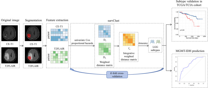 Figure 1
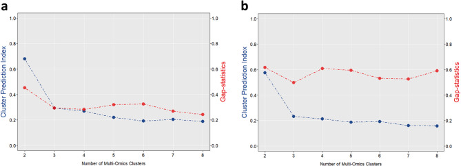 Figure 2
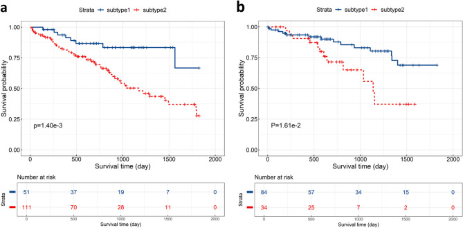 Figure 3
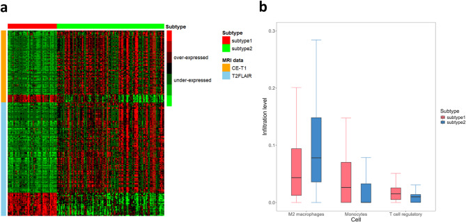 Figure 4
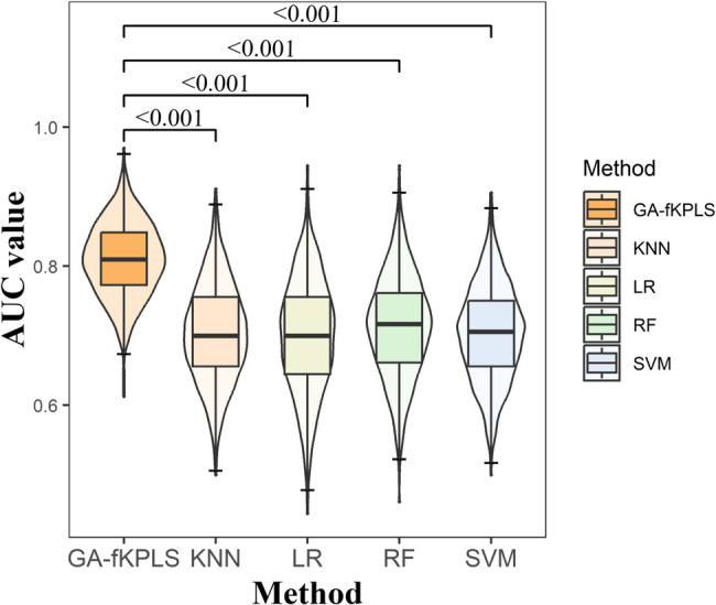 Figure 5
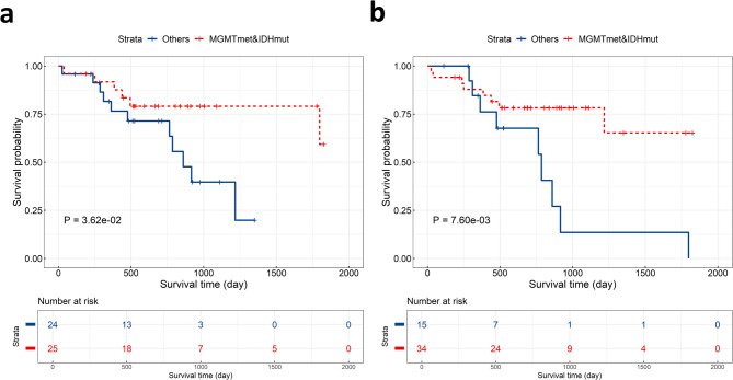 Figure 6
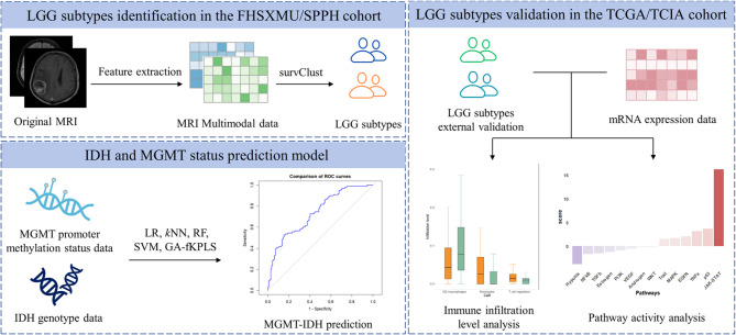 Figure 7
- —National Natural Science Foundation of China
- —https://doi.org/10.13039/501100019447Applied Basic Research Project of Shanxi Province, China
- —Shanxi Province Research Funding Project for Returned Overseas Scholars
- —Shanxi Province Higher Education “Billion Project” Science and Technology Guidance Project
Peer Reviews
No public reviews on file for this paper yet. If you reviewed it on a platform where reviews are public (OpenReview, ICLR, NeurIPS, ICML), you can paste yours below so the community can read it here.
Videos
No videos yet. Explain this paper in a talk, walkthrough, or lecture? Add one.
Taxonomy
TopicsGlioma Diagnosis and Treatment · MRI in cancer diagnosis · Advanced Neuroimaging Techniques and Applications
Background
Low-grade gliomas (LGG), defined as World Health Organization (WHO) grades II and III gliomas, are the most common diffuse and infiltrative primary malignant brain tumors in adults [1–3]. The histopathological classification of LGG has traditionally guided clinical management decisions. However, due to the high heterogeneity of tumors, even when LGG patients at the same histological stages receive the same treatment, their responses and clinical outcomes can vary widely [4, 5]. There is an urgent need to employ robust methods that can identify high-risk LGG phenotypic subtypes and uncover potential therapeutic targets, facilitating precision diagnosis, intervention, and clinical decision-making for LGG patients.
Magnetic resonance imaging (MRI) is commonly used for preoperative evaluation of LGG due to its non-invasive nature and widespread clinical application [6]. MRI encompasses modalities such as post-contrast enhanced T1-weighted (CE-T1) imaging and T2-weighted fluid attenuation inversion recovery (T2FLAIR) imaging, each of which can provide distinct information about the tumor. CE-T1 enables precise tumor localization and size assessment by enhancing the visibility of angiogenesis-associated abnormal areas using contrast agents like gadolinium. CE-T1 is particularly useful in identifying and delineating the boundaries of LGG lesions, especially for surgical planning and tumor volumetry [7]. T2FLAIR combines T2-weighted imaging with fluid-attenuated inversion recovery sequences, effectively displaying edema and abnormal signals in surrounding tissues [8]. It is particularly suited for visualizing the infiltrative growth patterns around tumors and their boundary with normal brain tissue, facilitating the evaluation of tumor extent and potential surgical margins. While each MRI modality has specific advantages in LGG characterization, the multimodal MRI data integration enables more comprehensive tumor profiling, facilitating development of precise individualized treatment strategies and providing reliable prognostic evaluation [9, 10].
Current glioma subtype identification primarily employs conventional clustering methods (e.g., k-means, hierarchical clustering) [11–13]. Multimodal data integration clustering methods allow joint analysis of multimodal data, enhancing information utilization for more comprehensive biological insights [14]. Among existing multimodal data integration methods, most fail to model patient survival outcomes as the optimization objective, instead evaluating prognostic differences through post hoc subtype analysis [15, 16]. This results in the identified molecular subtypes potentially lacking survival differences, thereby limiting their clinical translational value. Unlike traditional multimodal data integration clustering methods, survClust is an outcome-weighted integrative clustering algorithm that integrates patient outcome data during the clustering process to identify cancer subtypes with prognostic significance [17]. The algorithm constructs an outcome-associated distance matrix that downweights features with no relevance to the outcome, thereby enabling accurate identification of cancer subtypes with significant survival differences. Simultaneously, adopting K-fold cross-validation, the survClust method avoids “overfitting” that occurs when using survival data in both model construction and prognosis evaluation [17].
In this study, we aim to identify LGG phenotypic subtypes using the survClust method based on preoperative multimodal MRI data from the First Hospital of Shanxi Medical University (FHSXMU) and Shanxi Provincial People’s Hospital (SPPH), and validate them in The Cancer Genome Atlas (TCGA)/The Cancer Imaging Archive (TCIA) dataset. Furthermore, we will explore biomarkers associated with LGG phenotypic subtypes, revealing the main driving factors of disease development and facilitating targeted interventions and prognostic evaluation in LGG patients.
Methods
Statistical analyses were performed using R software (version 4.3.2). The significance level \documentclass[12pt]{minimal} \usepackage{amsmath} \usepackage{wasysym} \usepackage{amsfonts} \usepackage{amssymb} \usepackage{amsbsy} \usepackage{mathrsfs} \usepackage{upgreek} \setlength{\oddsidemargin}{-69pt} \begin{document}$$\:\alpha\:=0.05$$\end{document} . The conceptual framework of this study is presented in Fig. 1.Fig. 1. The overview of this study. We first extracted CE-T1 and T2FLAIR features from brain MRI images of LGG patients from FHSXMU/SPPH cohort and TCGA/TCIA cohort. In the FHSXMU/SPPH cohort, we identified two LGG phenotypic subtypes using SurvClust method based on multimodal MRI data. Then we performed predictive analysis of IDH mutations combined with MGMT promoter methylation, using significant MRI features identified between the subtypes. The identified phenotypic subtypes were subsequently validated in an external dataset (the TCGA/TCIA cohort) using SurvClust method based on significant MRI features identified between the subtypes
Patients
This study collected glioma patients from hospitals, including the FHSXMU and SPPH (344 cases), and the TCGA [18] (https://portal.gdc.cancer.gov/)/TCI/TCI)A [19] (https://nbia.cancerimagingarchive.net/nbia-search/) project (208 cases). The inclusion criteria for LGG patients of this study are as follows: (i) pathologically confirmed WHO grade Ⅱ and grade Ⅲ glioma according to the 2021 WHO standards; (ii) availability of preoperative three-week MRI data, including CE-T1 and T2FLAIR images; (iii) clear genotype of isocitrate dehydrogenase (IDH) and O6-methylguanine-DNA methyltransferase (MGMT) promoter methylation status; (iv) follow-up time exceeded 2 years or occurred an endpoint event. Overall survival is calculated from the time of postoperative pathological diagnosis until death or the last follow-up. The exclusion criteria were as follows: (1) targeted treatment (including conservative treatment, radiotherapy and chemotherapy) had been received before surgery; (2) severe poor image quality or image motion artifacts; (3) lack of postoperative follow-up or loss to follow-up. Ultimately, 280 patients met these criteria, including 162 patients from the FHSXMU/SPPH cohort and 118 patients from the TCGA/TCIA cohort.
MRI feature extraction and quantification
In the FHSXMU/SPPH cohort, all preoperative MRI images were acquired from 3.0-T scanners. The detailed scanning parameters are shown in the supplementary information (1). In the TCGA/TCIA cohort, preoperative MRI was acquired from TCIA project. Since the images from the TCGA/TCIA database come from different MRI devices and acquisition protocols, and there are also differences in MRI devices and acquisition protocols between the FHSXMU and SPPH datasets, we resampled all MRI images to ensure the spatial resolution and intensity of the images are comparable. This process eliminates the interference caused by inconsistent spatial resolution due to different MRI device models, and we performed intensity normalization using the min-max normalization method. This process was implemented using the SimpleITK library (https://github.com/SimpleITK/SimpleITK) in Python (version 3.10.4).
The T2FLAIR images were registered to the corresponding CE-T1 images through affine transformation using the FSL software (FMRIB Software Library, FSL, https://fsl.fmrib.ox.ac.uk/fsl/fslwiki/FSL). We chose CE-T1 as the primary reference for segmentation due to its high spatial resolution and clinical utility in defining tumor boundaries, which is critical for surgical planning and volumetric assessment. For the enhanced tumor ROI, the border was defined by the enhanced rim, and the tumor region of interest (ROI) was outlined on CE-T1 images and then transferred to T2FLAIR images. For unenhanced tumors, the tumor intensity on CE-T1 MRI images was lower than the surrounding peritumoral edema, and the ROI was similarly outlined on CE-T1 images and transferred to T2FLAIR. If the tumor border was unclear on both CE-T1 and T2FLAIR MRI images, DWI and ADC MRI images (if available) were used to help define the boundaries. Two radiologists, with varying years of experience in brain MRI diagnosis and without prior knowledge of the patients’ clinical data or other imaging results, imported the CE-T1 images into ITK-SNAP software (http://www.itksnap.org, version 3.8.0) for image segmentation. They first converted the images from DICOM to NIFTI format and then performed image segmentation. The tumor ROI was outlined slice by slice either manually or with semi-automated computer-assisted methods, to obtain the three-dimensional volume of interest (VOI). Subsequently, the resulting VOI images were imported into FAE software [20] (https://github.com/salan668/FAE, version 0.5.6) for MRI feature extraction. The extracted features include 18 first order features, 14 shape features, and 75 texture features. Texture features consist of 24 Gray Level Co-occurrence Matrix (GLCM) features, 14 Gray Level Dependence Matrix (GLDM) features, 16 Gray Level Run-Length Matrix (GLRLM) features, 16 Gray Level Size Zone Matrix (GLSZM) features, and 5 Neighboring Gray Tone Difference Matrix (NGTDM) features. Simultaneously, six types of image filters—wavelet transform, square, square root, logarithm, exponential, and gradient—were used for preprocessing the original images.
Finally, in the FHSXMU/SPPH cohort, a total of 1688 MRI features were extracted from each of the CE-T1 and T2FLAIR images. Two variables (T1c_lbp-3D-m1_firstorder_Minimum and T1c_lbp-3D-m2_firstorder_Minimum) of CE-T1 were excluded due to their values were entirely zero, retaining 1686 features. Similarly, two variables (FLAIR_lbp-3D-m1_firstorder_Minimum and FLAIR_lbp-3D-m2_firstorder_Minimum) of T2FLAIR were excluded because 98.15% of their values were zero, leaving 1686 features. We obtained the same MRI features from the TCGA/TCIA cohort. Subsequently, both CE-T1 and T2FLAIR data were standardized for further analysis.
To evaluate feature reproducibility, MRI features extracted from ROIs were tested for intra- and inter-observer (intraclass correlation coefficient, ICC) agreement using repeated segmentations by one radiologist (> 3-month interval) on 30 randomly selected LGG MRI cases. The MRI features demonstrated excellent reproducibility, with intra-observer ICC values (median = 0.88, IQR: [0.86–0.91]) and inter-observer ICCs (median = 0.85, IQR: [0.82–0.87]). Additionally, 86.7% of tested features showed ICC > 0.75.
IDH genotype and MGMT promoter methylation status data
For the FHSXMU/SPPH cohort, IDH mutation status was analyzed by Sanger sequencing, while MGMT promoter methylation was evaluated via pyrosequencing [21]. The details of test methods are described in our prior publication [22]. For patients in the TCGA/TCIA cohort, IDH genotype and MGMT promoter methylation status data were obtained from the Genomic Data Commons Data Portal.
Acquisition and processing of mRNA expression data
The mRNA expression data of the TCGA/TCIA cohort were downloaded from the TCGA project. We excluded non-protein-coding genes, averaged duplicate genes and samples (retaining only one for each duplicate), and removed genes and samples with over 30% zero expression. To refine the distribution of gene expression data for more robust statistical analysis, we transformed gene expression values by \documentclass[12pt]{minimal} \usepackage{amsmath} \usepackage{wasysym} \usepackage{amsfonts} \usepackage{amssymb} \usepackage{amsbsy} \usepackage{mathrsfs} \usepackage{upgreek} \setlength{\oddsidemargin}{-69pt} \begin{document}$$\:{\text{log}}_{2}(x+1)$$\end{document} . Finally, we obtained the mRNA expression data including 19,938 genes.
The survClust method
The survClust algorithm (https://github.com/arorarshi/survClust) constructs a weighted distance matrix that down-weights MRI features unrelated to the outcome of interest [17]. Let \documentclass[12pt]{minimal} \usepackage{amsmath} \usepackage{wasysym} \usepackage{amsfonts} \usepackage{amssymb} \usepackage{amsbsy} \usepackage{mathrsfs} \usepackage{upgreek} \setlength{\oddsidemargin}{-69pt} \begin{document}$$\:{X}_{m}$$\end{document} be the \documentclass[12pt]{minimal} \usepackage{amsmath} \usepackage{wasysym} \usepackage{amsfonts} \usepackage{amssymb} \usepackage{amsbsy} \usepackage{mathrsfs} \usepackage{upgreek} \setlength{\oddsidemargin}{-69pt} \begin{document}$$\:m\text{t}\text{h}$$\end{document} data type with dimensions \documentclass[12pt]{minimal} \usepackage{amsmath} \usepackage{wasysym} \usepackage{amsfonts} \usepackage{amssymb} \usepackage{amsbsy} \usepackage{mathrsfs} \usepackage{upgreek} \setlength{\oddsidemargin}{-69pt} \begin{document}$$\:{N}_{m}\times\:{p}_{m}$$\end{document} , where \documentclass[12pt]{minimal} \usepackage{amsmath} \usepackage{wasysym} \usepackage{amsfonts} \usepackage{amssymb} \usepackage{amsbsy} \usepackage{mathrsfs} \usepackage{upgreek} \setlength{\oddsidemargin}{-69pt} \begin{document}$$\:{N}_{m}$$\end{document} is the number of samples and \documentclass[12pt]{minimal} \usepackage{amsmath} \usepackage{wasysym} \usepackage{amsfonts} \usepackage{amssymb} \usepackage{amsbsy} \usepackage{mathrsfs} \usepackage{upgreek} \setlength{\oddsidemargin}{-69pt} \begin{document}$$\:{p}_{m}$$\end{document} is the number of features, with rows representing samples and columns representing features. The univariable Cox proportional hazards model fitted for each feature is calculated as:
\documentclass[12pt]{minimal} \usepackage{amsmath} \usepackage{wasysym} \usepackage{amsfonts} \usepackage{amssymb} \usepackage{amsbsy} \usepackage{mathrsfs} \usepackage{upgreek} \setlength{\oddsidemargin}{-69pt} \begin{document}$$\:\text{h}\left(t|{x}_{p}\right)={h}_{0}\times\:exp\left({x}_{j}^{T}*\beta\:\right)$$\end{document}Here, \documentclass[12pt]{minimal} \usepackage{amsmath} \usepackage{wasysym} \usepackage{amsfonts} \usepackage{amssymb} \usepackage{amsbsy} \usepackage{mathrsfs} \usepackage{upgreek} \setlength{\oddsidemargin}{-69pt} \begin{document}$$\:t$$\end{document} denotes survival time, \documentclass[12pt]{minimal} \usepackage{amsmath} \usepackage{wasysym} \usepackage{amsfonts} \usepackage{amssymb} \usepackage{amsbsy} \usepackage{mathrsfs} \usepackage{upgreek} \setlength{\oddsidemargin}{-69pt} \begin{document}$$\:{x}_{j}$$\end{document} refers to the \documentclass[12pt]{minimal} \usepackage{amsmath} \usepackage{wasysym} \usepackage{amsfonts} \usepackage{amssymb} \usepackage{amsbsy} \usepackage{mathrsfs} \usepackage{upgreek} \setlength{\oddsidemargin}{-69pt} \begin{document}$$\:j$$\end{document} -th column of matrix \documentclass[12pt]{minimal} \usepackage{amsmath} \usepackage{wasysym} \usepackage{amsfonts} \usepackage{amssymb} \usepackage{amsbsy} \usepackage{mathrsfs} \usepackage{upgreek} \setlength{\oddsidemargin}{-69pt} \begin{document}$$\:X$$\end{document} with length \documentclass[12pt]{minimal} \usepackage{amsmath} \usepackage{wasysym} \usepackage{amsfonts} \usepackage{amssymb} \usepackage{amsbsy} \usepackage{mathrsfs} \usepackage{upgreek} \setlength{\oddsidemargin}{-69pt} \begin{document}$$\:N$$\end{document} , \documentclass[12pt]{minimal} \usepackage{amsmath} \usepackage{wasysym} \usepackage{amsfonts} \usepackage{amssymb} \usepackage{amsbsy} \usepackage{mathrsfs} \usepackage{upgreek} \setlength{\oddsidemargin}{-69pt} \begin{document}$$\:{h}_{0}$$\end{document} is the baseline hazard function, \documentclass[12pt]{minimal} \usepackage{amsmath} \usepackage{wasysym} \usepackage{amsfonts} \usepackage{amssymb} \usepackage{amsbsy} \usepackage{mathrsfs} \usepackage{upgreek} \setlength{\oddsidemargin}{-69pt} \begin{document}$$\:\beta\:$$\end{document} represents the regression coefficient, and \documentclass[12pt]{minimal} \usepackage{amsmath} \usepackage{wasysym} \usepackage{amsfonts} \usepackage{amssymb} \usepackage{amsbsy} \usepackage{mathrsfs} \usepackage{upgreek} \setlength{\oddsidemargin}{-69pt} \begin{document}$$\:exp\left(\beta\:\right)$$\end{document} indicates the hazard ratio (HR).
The absolute value of the HR on the logarithmic scale from a univariate Cox proportional hazards model, fitted for the survival outcome (time) with each feature, is considered as the feature weight \documentclass[12pt]{minimal} \usepackage{amsmath} \usepackage{wasysym} \usepackage{amsfonts} \usepackage{amssymb} \usepackage{amsbsy} \usepackage{mathrsfs} \usepackage{upgreek} \setlength{\oddsidemargin}{-69pt} \begin{document}$$\:{w}_{k}$$\end{document} . Then we can obtain the feature-weighted matrix \documentclass[12pt]{minimal} \usepackage{amsmath} \usepackage{wasysym} \usepackage{amsfonts} \usepackage{amssymb} \usepackage{amsbsy} \usepackage{mathrsfs} \usepackage{upgreek} \setlength{\oddsidemargin}{-69pt} \begin{document}$$\:W=\text{d}\text{i}\text{a}\text{g}\left\{{w}_{1},{w}_{2},\cdots\:,{w}_{k}\right\}$$\end{document} . The weighted distance matrix \documentclass[12pt]{minimal} \usepackage{amsmath} \usepackage{wasysym} \usepackage{amsfonts} \usepackage{amssymb} \usepackage{amsbsy} \usepackage{mathrsfs} \usepackage{upgreek} \setlength{\oddsidemargin}{-69pt} \begin{document}$$\:{d}_{w}$$\end{document} , for a pair of two samples \documentclass[12pt]{minimal} \usepackage{amsmath} \usepackage{wasysym} \usepackage{amsfonts} \usepackage{amssymb} \usepackage{amsbsy} \usepackage{mathrsfs} \usepackage{upgreek} \setlength{\oddsidemargin}{-69pt} \begin{document}$$\:\text{a}$$\end{document} and \documentclass[12pt]{minimal} \usepackage{amsmath} \usepackage{wasysym} \usepackage{amsfonts} \usepackage{amssymb} \usepackage{amsbsy} \usepackage{mathrsfs} \usepackage{upgreek} \setlength{\oddsidemargin}{-69pt} \begin{document}$$\:\text{b}$$\end{document} , is calculated as follows:
\documentclass[12pt]{minimal} \usepackage{amsmath} \usepackage{wasysym} \usepackage{amsfonts} \usepackage{amssymb} \usepackage{amsbsy} \usepackage{mathrsfs} \usepackage{upgreek} \setlength{\oddsidemargin}{-69pt} \begin{document}$$\:{d}_{w}\left(a,b\right)=\sqrt{{\left(a-b\right)}^{T}W\left(a-b\right)}$$\end{document}Then we calculate the integrated weighted distance matrix:
\documentclass[12pt]{minimal} \usepackage{amsmath} \usepackage{wasysym} \usepackage{amsfonts} \usepackage{amssymb} \usepackage{amsbsy} \usepackage{mathrsfs} \usepackage{upgreek} \setlength{\oddsidemargin}{-69pt} \begin{document}$${I}_{w}=\sum_{m=1}^{M}{\gamma}_{m}{D}_{m}$$\end{document}\documentclass[12pt]{minimal} \usepackage{amsmath} \usepackage{wasysym} \usepackage{amsfonts} \usepackage{amssymb} \usepackage{amsbsy} \usepackage{mathrsfs} \usepackage{upgreek} \setlength{\oddsidemargin}{-69pt} \begin{document}$$\:{D}_{m}(m=\text{1,2},\cdots\:M)$$\end{document} is the \documentclass[12pt]{minimal} \usepackage{amsmath} \usepackage{wasysym} \usepackage{amsfonts} \usepackage{amssymb} \usepackage{amsbsy} \usepackage{mathrsfs} \usepackage{upgreek} \setlength{\oddsidemargin}{-69pt} \begin{document}$$\:m\text{t}\text{h}$$\end{document} weighted distance matrix, and \documentclass[12pt]{minimal} \usepackage{amsmath} \usepackage{wasysym} \usepackage{amsfonts} \usepackage{amssymb} \usepackage{amsbsy} \usepackage{mathrsfs} \usepackage{upgreek} \setlength{\oddsidemargin}{-69pt} \begin{document}$$\:{\gamma\:}_{m}=\frac{1}{M}\forall\:m$$\end{document} . \documentclass[12pt]{minimal} \usepackage{amsmath} \usepackage{wasysym} \usepackage{amsfonts} \usepackage{amssymb} \usepackage{amsbsy} \usepackage{mathrsfs} \usepackage{upgreek} \setlength{\oddsidemargin}{-69pt} \begin{document}$$\:{I}_{w}$$\end{document} is then clustered by k-means [23]. To avoid overfitting and achieve more generalizable solutions, survClust employs K-fold cross-validation [17]. Final subtype labels were determined by consensus voting across 50 rounds of cross-validation.
In this study, we obtained the integrated weighted distance based on multimodal MRI data through the aforementioned steps. The cluster initialization was performed using the k-means + + algorithm [24], with 100 random starts to ensure stability. The clustering process was set to run for a maximum of 100 iterations, with convergence defined as centroid displacements < 1.00e-5 between consecutive iterations. We used 3-fold cross-validation, selected based on survClust’s validation framework [17], which demonstrates strong subtype stability with smaller sample sizes.
Estimating the optimal number of clusters
Clustering Prediction Index (CPI) estimates the optimal cluster number ( \documentclass[12pt]{minimal} \usepackage{amsmath} \usepackage{wasysym} \usepackage{amsfonts} \usepackage{amssymb} \usepackage{amsbsy} \usepackage{mathrsfs} \usepackage{upgreek} \setlength{\oddsidemargin}{-69pt} \begin{document}$$\:{k}_{1}$$\end{document} ) by resampling based cross-validation technique [25]. It works by splitting the data into training and test sets, repeating this to generate multiple pairs. A clustering algorithm trains on the training data to find cluster centers, which then assign test samples to the nearest cluster. The CPI is computed as the average within-cluster sum of squares across all test samples, calculated as follows:
\documentclass[12pt]{minimal} \usepackage{amsmath} \usepackage{wasysym} \usepackage{amsfonts} \usepackage{amssymb} \usepackage{amsbsy} \usepackage{mathrsfs} \usepackage{upgreek} \setlength{\oddsidemargin}{-69pt} \begin{document}$$\text{CPI}\left(k\right)=\frac1m\sum_{i=1}^m\sum_{x\in X_{n_2\times p_i}^i}\left\|x-C_i^{\left(k1\right)}\left(x\right)\right\|^2$$\end{document}Here, \documentclass[12pt]{minimal} \usepackage{amsmath} \usepackage{wasysym} \usepackage{amsfonts} \usepackage{amssymb} \usepackage{amsbsy} \usepackage{mathrsfs} \usepackage{upgreek} \setlength{\oddsidemargin}{-69pt} \begin{document}$$\:m$$\end{document} denotes the number of data splits, and \documentclass[12pt]{minimal} \usepackage{amsmath} \usepackage{wasysym} \usepackage{amsfonts} \usepackage{amssymb} \usepackage{amsbsy} \usepackage{mathrsfs} \usepackage{upgreek} \setlength{\oddsidemargin}{-69pt} \begin{document}$$\:{C}_{i}^{\left(k1\right)}\left(x\right)$$\end{document} represents the assigned cluster centroid for the test sample \documentclass[12pt]{minimal} \usepackage{amsmath} \usepackage{wasysym} \usepackage{amsfonts} \usepackage{amssymb} \usepackage{amsbsy} \usepackage{mathrsfs} \usepackage{upgreek} \setlength{\oddsidemargin}{-69pt} \begin{document}$$x$$\end{document} .
Gap-statistics determines the optimal number of clusters ( \documentclass[12pt]{minimal} \usepackage{amsmath} \usepackage{wasysym} \usepackage{amsfonts} \usepackage{amssymb} \usepackage{amsbsy} \usepackage{mathrsfs} \usepackage{upgreek} \setlength{\oddsidemargin}{-69pt} \begin{document}$$\:{k}_{2}$$\end{document} ) by comparing the observed within-cluster sum of squares( \documentclass[12pt]{minimal} \usepackage{amsmath} \usepackage{wasysym} \usepackage{amsfonts} \usepackage{amssymb} \usepackage{amsbsy} \usepackage{mathrsfs} \usepackage{upgreek} \setlength{\oddsidemargin}{-69pt} \begin{document}$$\:{W}_{k2}$$\end{document} ) with its expected value under null reference distribution [26]. The Gap-statistics is maximized as follows:
\documentclass[12pt]{minimal} \usepackage{amsmath} \usepackage{wasysym} \usepackage{amsfonts} \usepackage{amssymb} \usepackage{amsbsy} \usepackage{mathrsfs} \usepackage{upgreek} \setlength{\oddsidemargin}{-69pt} \begin{document}$$\begin{aligned}\:{\text{Gap}}_{n}\left(k\right)=&{E}_{n}^{*}\left\{\text{log}\left(\sum\:_{r=1}^{k2}\frac{1}{2{n}_{r}}\sum\:_{i,i{\prime\:}\in\:{C}_{r}}{d}_{ii{\prime\:}}\right)\right\}\\&-\text{log}\left(\sum\:_{r=1}^{k2}\frac{1}{2{n}_{r}}\sum\:_{i,i{\prime\:}\in\:{C}_{r}}{d}_{ii{\prime\:}}\right)\end{aligned}$$\end{document}Here, \documentclass[12pt]{minimal} \usepackage{amsmath} \usepackage{wasysym} \usepackage{amsfonts} \usepackage{amssymb} \usepackage{amsbsy} \usepackage{mathrsfs} \usepackage{upgreek} \setlength{\oddsidemargin}{-69pt} \begin{document}$$\:n$$\end{document} represents the sample size, \documentclass[12pt]{minimal} \usepackage{amsmath} \usepackage{wasysym} \usepackage{amsfonts} \usepackage{amssymb} \usepackage{amsbsy} \usepackage{mathrsfs} \usepackage{upgreek} \setlength{\oddsidemargin}{-69pt} \begin{document}$$\:{C}_{r}$$\end{document} indicates each cluster, \documentclass[12pt]{minimal} \usepackage{amsmath} \usepackage{wasysym} \usepackage{amsfonts} \usepackage{amssymb} \usepackage{amsbsy} \usepackage{mathrsfs} \usepackage{upgreek} \setlength{\oddsidemargin}{-69pt} \begin{document}$$\:i$$\end{document} and \documentclass[12pt]{minimal} \usepackage{amsmath} \usepackage{wasysym} \usepackage{amsfonts} \usepackage{amssymb} \usepackage{amsbsy} \usepackage{mathrsfs} \usepackage{upgreek} \setlength{\oddsidemargin}{-69pt} \begin{document}$$\:i{\prime\:}$$\end{document} are the observations within the cluster, and \documentclass[12pt]{minimal} \usepackage{amsmath} \usepackage{wasysym} \usepackage{amsfonts} \usepackage{amssymb} \usepackage{amsbsy} \usepackage{mathrsfs} \usepackage{upgreek} \setlength{\oddsidemargin}{-69pt} \begin{document}$$d$$\end{document} measures their squared Euclidean distance.
In this study, the optimal cluster number was selected at the maximum sum of CPI and Gap-statistics [27].
Identification and evaluation of LGG phenotypic subtypes
For the FHSXMU/SPPH cohort, we identified LGG phenotypic subtypes based on multimodal MRI data using the survClust method. The Kruskal-Wallis H-test was used to select MRI features with significant differences between the different subtypes in the FHSXMU/SPPH cohort, followed by a false discovery rate (FDR) adjustment ( \documentclass[12pt]{minimal} \usepackage{amsmath} \usepackage{wasysym} \usepackage{amsfonts} \usepackage{amssymb} \usepackage{amsbsy} \usepackage{mathrsfs} \usepackage{upgreek} \setlength{\oddsidemargin}{-69pt} \begin{document}$$\:{P}_{adj}<0.05$$\end{document} ). Subsequently, these selected features were matched by name with MRI features from the TCGA/TCIA cohort. Based on these matched MRI features, the survClust method was used to subtype patients in the TCGA/TCIA cohort.
With a five-year cutoff, we analyzed survival differences among patients of different subtypes using Kaplan-Meier survival analysis and log-rank test. We conducted differential analysis for various factors between different subtypes, with continuous variables analyzed using the Kruskal-Wallis H-test and categorical variables evaluated using the Chi-Square test. In the FHSXMU/SPPH cohort, we employed a multivariate Cox proportional hazards model to evaluate prognostic differences among LGG phenotypic subtypes and identify the high-risk subtype, adjusting for age, gender, and pathological stage. To ensure the reliability of the Cox model, we performed an evaluation of all variables in the Cox model using the Schoenfeld residuals test, and calculated the Events Per Variable (EPV).
Differential and enrichment analysis of MRI features
For the selected differential MRI features after the Kruskal-Wallis H-test with an FDR-adjusted P-value ( \documentclass[12pt]{minimal} \usepackage{amsmath} \usepackage{wasysym} \usepackage{amsfonts} \usepackage{amssymb} \usepackage{amsbsy} \usepackage{mathrsfs} \usepackage{upgreek} \setlength{\oddsidemargin}{-69pt} \begin{document}$$\:{P}_{adj}<0.05$$\end{document} ), we conducted enrichment analysis for CE-T1 and T2FLAIR features across LGG phenotypic subtypes using the hypergeometric test with an FDR-adjusted P-value ( \documentclass[12pt]{minimal} \usepackage{amsmath} \usepackage{wasysym} \usepackage{amsfonts} \usepackage{amssymb} \usepackage{amsbsy} \usepackage{mathrsfs} \usepackage{upgreek} \setlength{\oddsidemargin}{-69pt} \begin{document}$$\:{P}_{adj}<0.05$$\end{document} ).
To select features significantly enriched for distinct LGG phenotypic subtypes, a feature was considered over-expressed or under-expressed if its standardized Z-scores exceeded 0.6 or lower than − 0.6. For each subtype, the hypergeometric test was applied to evaluate significant enrichment of either over-expressed or under-expressed features. To identify most representative features of a given subtype, stringent criteria were applied: only features significantly enriched in at least 2/3 of samples within a subtype and in fewer than 1/3 of samples in any other subtype were selected.
Immune infiltration analysis and pathway activity analysis
We conducted immune infiltration analysis and pathway activity analysis using mRNA expression data from the TCGA/TCIA cohort. Using the ‘BIOR’ package, we estimated tumor cell composition and performed Kruskal-Wallis H-tests with an FDR-adjusted P-value ( \documentclass[12pt]{minimal} \usepackage{amsmath} \usepackage{wasysym} \usepackage{amsfonts} \usepackage{amssymb} \usepackage{amsbsy} \usepackage{mathrsfs} \usepackage{upgreek} \setlength{\oddsidemargin}{-69pt} \begin{document}$$\:{P}_{adj}<0.05$$\end{document} ) to identify immune cells exhibiting significantly different infiltration levels among different subtypes.
The pathway activity analysis was conducted through the following steps: (1) differentially expressed genes (DEGs) between different subtypes in the TCGA/TCIA cohort were identified using the “limma” package (version 3.58.1). (2) Using the “decoupleR” package (version 2.9.7), the gene weights and P values for 14 pathways were retrieved from the PROGENy database and the top 100 most significant genes (ranked by P value) were retained for per pathway. (3) A multivariate linear model (MLM) was applied to the DEGs to estimate pathway activity score. For each sample in the TCGA/TCIA cohort, the MLM predicted gene expression based on the pathway-gene interaction weights across 14 pathways. The resulting slope t-values represented the pathway activity scores, where positive t-values indicated pathway activation and negative t-values suggested inactivation.
Predictive modeling of IDH mutation combined with MGMT promoter methylation
IDH mutation and MGMT promoter methylation are frequently observed in LGG [28]. Previous studies have demonstrated that the glioma patients with IDH mutation combined with MGMT promoter methylation have a longer overall survival (OS) and/or progression-free survival (PFS) [29, 30]. Therefore, precise identification of patients with combined IDH mutation and MGMT promoter methylation is critical for treatment decision-making and prognosis evaluation in glioma patients. The predictive model based on multimodal MRI for IDH mutation and MGMT promoter methylation status in glioma has potential as a non-invasive auxiliary diagnostic tool [9, 31].
In this study, patients with both MGMT promoter methylation and IDH mutation were grouped together as “MGMTmet&IDHmut” group, while all others were assigned to “Others” group, labeled as the MGMT-IDH variable.
Both CE-T1 and T2FLAIR data contain numerous features, most of which may be unrelated to predicting MGMT-IDH. Therefore, feature selection is necessary to optimize predictive model performance. We combined the selected differential MRI features after the Kruskal-Wallis H-test into a matrix, and conducted a stability feature selection on the matrix using a penalized logistic regression [32]. The matrix was randomly split into training and testing datasets with an 8:2 ratio. Then, we used L1-penalized logistic regression on the training data to select features, while selected the optimal lambda value using 10-fold cross-validation. We recorded the feature selection results from 100 random splits (seed = 1-100) of the samples, and select MRI features with a frequency of occurrence ≥ 10% as the final selected features. Ridge regression (L2 penalty) can serve as an alternative shrinkage method, but it retains all features, potentially keeping noise variables. In our study, we prefer L1-penalized logistic regression for feature selection, as it can shrink the coefficients of irrelevant features to zero, achieving sparsity and interpretability. This aligns directly with our goal of predicting MGMT-IDH status using a minimal set of MRI features.
Then, using final selected MRI features as predictors, we constructed MGMT-IDH prediction models based on partial least squares with the genetic algorithm (GA-fKPLS) [33], logistic regression (LR) [34], random forest (RF) [35], support vector machine (SVM) [36], k-nearest neighbor (kNN) [37].
In this study, patients from the FHSXMU/SPPH cohort were split into two non-overlapping subsets, with 80% used for training and 20% for testing. To enhance the stability and reproducibility of the results, the random splitting process was repeated 1000 times under different seed numbers (seed numbers = 1-1000). To validate the model’s effectiveness, we conducted comprehensive external validation using the TCGA/TCIA cohort, employing the same feature selection and modeling methods as for the FHSXMU/SPPH cohort.
We employed eight evaluation criteria to assess the predictive performance of the five models, including the area under the curve (AUC), sensitivity (Se), specificity (Sp), accuracy (ACC), Youden index, F-measure, Matthews correlation coefficient (MCC), and G-means. The final performance of each model was evaluated based on the average values of these eight metrics across the 1000 independent data splits. Among these, the MCC and AUC were the main criteria used for model evaluation, as they provide a more comprehensive evaluation of model performance. To further illustrate the performance of the five models, we used one-way analysis of variance followed by Dunnett’s multiple comparison test to compare the highest AUC value with the AUC values of the other four models.
Results
Patient characteristics
Basic characteristics of patients from the FHSXMU/SPPH cohort and the TCGA/TCIA cohort are shown in Table 1.
Table 1. Patient characteristics in the FHSXMU/SPPH cohort and TCGA/TCIA cohortCharacteristicFHSXMU/SPPH cohort (n = 162)TCGA/TCIA cohort (n = 118)Sex n (%) Female86(53.09)55(46.61) Male76(46.91)63(53.39)Age n (%) <35 years76(46.91)27(22.88) ≥35 years86(53.09)91(77.12)Pathological grade n (%) WHO II82(50.62)54(45.76) WHO III80(49.38)64(54.24)MGMT promoter status n (%) Unmethylation44(27.16)18(15.25) Methylation118(72.84)100(84.75)IDH genotype n (%) Wild type73(45.06)24(20.34) Mutation89(54.94)94(79.66)Vital status n (%) Death106(65.43)32(27.12) Survival56(34.57)86(72.88)Tumor volume (cm^3^, mean±SD)38.10±35.1342.92±53.59
Identification of two LGG phenotypic subtypes
Since the sum of CPI and Gap-statistic was maximum when the number of clusters was 2, we decided 2 as the optimal number of clusters for the FHSXMU/SPPH cohort (Fig. 2a). In the FHSXMU/SPPH cohort, based on multimodal MRI data, two LGG phenotypic subtypes (subtype 1 with 51 patients and subtype 2 with 111 patients) were successfully identified using the survClust method. Subtype 1 had 9 deaths out of 51 patients (17.6%), while Subtype 2 had 47 deaths out of 111 patients (42.3%).
1333 CE-T1 features and 1273 T2FLAIR features with significant differences between the two subtypes were selected in the FHSXMU/SPPH cohort. The MRI features of TCGA/TCIA cohort were subsequently matched to the 2606 selected features based on their names. Because the sum of CPI and Gap-statistic was maximum when the number of clusters was 2, we selected 2 as the optimal number of clusters for the TCGA/TCIA cohort (Fig. 2b). Based on these matched MRI features, two subtypes were identified by survClust method, with 84 patients assigned to subtype 1 and 34 patients to subtype 2. In the TCGA/TCIA cohort, there were 20 deaths among the 84 patients in Subtype 1 and 12 deaths among the 34 patients in Subtype 2.
For both FHSXMU/SPPH cohort and TCGA/TCIA cohort, Kaplan-Meier survival analysis and log-rank test demonstrated significant prognostic difference ( \documentclass[12pt]{minimal} \usepackage{amsmath} \usepackage{wasysym} \usepackage{amsfonts} \usepackage{amssymb} \usepackage{amsbsy} \usepackage{mathrsfs} \usepackage{upgreek} \setlength{\oddsidemargin}{-69pt} \begin{document}$$\:P<0.05$$\end{document} ) between the two subtypes (Fig. 3).
Fig. 2. Results of CPI and Gap-statistic from 2 to 8 clusters in the FHSXMU/SPPH cohort (a) and TCGA/TCIA cohort (b)
Fig. 3. Kaplan-Meier curves of the LGG phenotypic subtypes in the FHSXMU/SPPH cohort (a) and TCGA/TCIA cohort (b)
Evaluation of LGG phenotypic subtypes
As presented in Table 2, in the FHSXMU/SPPH cohort, pathological grade, MGMT promoter status, IDH genotype, vital status, and tumor volume were statistically significant between the two subtypes ( \documentclass[12pt]{minimal} \usepackage{amsmath} \usepackage{wasysym} \usepackage{amsfonts} \usepackage{amssymb} \usepackage{amsbsy} \usepackage{mathrsfs} \usepackage{upgreek} \setlength{\oddsidemargin}{-69pt} \begin{document}$$\:P<0.05$$\end{document} ). The results of the multivariate Cox regression analysis, adjusted for age, gender, and pathological stage in the FHSXMU/SPPH cohort, are shown in Table 3. Patients in subtype 2 were 2.553 times higher risk of death compared to patients in subtype 1 ( \documentclass[12pt]{minimal} \usepackage{amsmath} \usepackage{wasysym} \usepackage{amsfonts} \usepackage{amssymb} \usepackage{amsbsy} \usepackage{mathrsfs} \usepackage{upgreek} \setlength{\oddsidemargin}{-69pt} \begin{document}$$\:P<0.05$$\end{document} ). Patients with WHO Ⅲ grade were 1.775 times higher risk of death compared to patients with WHO Ⅱ grade ( \documentclass[12pt]{minimal} \usepackage{amsmath} \usepackage{wasysym} \usepackage{amsfonts} \usepackage{amssymb} \usepackage{amsbsy} \usepackage{mathrsfs} \usepackage{upgreek} \setlength{\oddsidemargin}{-69pt} \begin{document}$$\:P<0.05$$\end{document} ). The Schoenfeld residuals test for all variables in the Cox model confirmed no significant time-dependent trends (Table S2).
Table 2. Baseline clinical and molecular data of FHSXMU/SPPH cohortCharacteristicSubtype 1 (n = 51)Subtype 2 (n = 111)dfχ^2^/H P Sex n (%) Female31(60.78)55(49.55) Male20(39.22)56(50.45)11.350.25Age n (%) <35 years8(15.69)22(19.82) ≥ 35 years43(84.31)89(80.18)10.170.68Pathological grade n (%) WHO II35(68.63)47(42.34) WHO III16(31.37)64(57.66)18.64 3.30e-3 MGMT promoter status n (%) Unmethylation8(15.69)36(32.43) Methylation43(84.31)75(67.57)14.14 0.04 IDH genotype n (%) Wild type15(29.41)58(52.25) Mutation36(70.59)53(47.75)16.47 0.01 Vital status n (%) Death9(17.65)47(42.34) Survival42(82.35)64(57.66)18.36 3.83e-3 Tumor volume (cm^3^, mean±SD)10.30±8.1150.87±35.41183.34 < 2.2e-16 MGMT-IDH n (%)MGMTmet&IDHmut35(68.63)44(39.64)Others16(31.37)67(60.36)110.62 1.12e-3 A P<0.05 was considered statistically significant. “df” represents degrees of freedom: \documentclass[12pt]{minimal} \usepackage{amsmath} \usepackage{wasysym} \usepackage{amsfonts} \usepackage{amssymb} \usepackage{amsbsy} \usepackage{mathrsfs} \usepackage{upgreek} \setlength{\oddsidemargin}{-69pt} \begin{document}$$Chi-Square\:test\:degrees\:of\:freedom\:=$$\end{document} \documentclass[12pt]{minimal} \usepackage{amsmath} \usepackage{wasysym} \usepackage{amsfonts} \usepackage{amssymb} \usepackage{amsbsy} \usepackage{mathrsfs} \usepackage{upgreek} \setlength{\oddsidemargin}{-69pt} \begin{document}$$\:(number\:of\:subtypes\:-\:1)\:\times\:\:(number\:of\:categories\:in\:variable\:2\:-\:1);$$\end{document} \documentclass[12pt]{minimal} \usepackage{amsmath} \usepackage{wasysym} \usepackage{amsfonts} \usepackage{amssymb} \usepackage{amsbsy} \usepackage{mathrsfs} \usepackage{upgreek} \setlength{\oddsidemargin}{-69pt} \begin{document}$$Kruskal-Wallis\:H-test\:degrees\:of\:freedom\:=\:number\:of\:subtypes\:-\:1$$\end{document}
Table 3. The multivariable Cox analysis for FHSXMU/SPPH cohortVariableBWaldSE P HR(95% CI)Subtype Subtype 20.9376.2760.374 0.012 2.553(1.226–5.315)Sex Female0.1590.330.2770.5661.173(0.681–2.020)Age ≥ 35 years0.5561.830.4110.1761.744(0.779–3.902)Pathological grade WHO III0.5743.860.292 0.049 1.775(1.001–3.145)Using subtype 1, male, < 35 years old and WHO II grade as the reference group. A \documentclass[12pt]{minimal} \usepackage{amsmath} \usepackage{wasysym} \usepackage{amsfonts} \usepackage{amssymb} \usepackage{amsbsy} \usepackage{mathrsfs} \usepackage{upgreek} \setlength{\oddsidemargin}{-69pt} \begin{document}$$\:P<0.05$$\end{document} was considered statistically significant. Cox model \documentclass[12pt]{minimal} \usepackage{amsmath} \usepackage{wasysym} \usepackage{amsfonts} \usepackage{amssymb} \usepackage{amsbsy} \usepackage{mathrsfs} \usepackage{upgreek} \setlength{\oddsidemargin}{-69pt} \begin{document}$$\:EPV\:=\:14$$\end{document}
As shown in Table 4, in the TCGA/TCIA cohort, IDH genotype and tumor volume were significantly different between the two subtypes ( \documentclass[12pt]{minimal} \usepackage{amsmath} \usepackage{wasysym} \usepackage{amsfonts} \usepackage{amssymb} \usepackage{amsbsy} \usepackage{mathrsfs} \usepackage{upgreek} \setlength{\oddsidemargin}{-69pt} \begin{document}$$\:P<0.05$$\end{document} ).
Table 4. Baseline clinical and molecular data of TCGA/TCIA cohortCharacteristicSubtype 1 (n = 84)Subtype 2 (n = 34)dfχ^2^/H P Sex n (%) Female39(46.43)16(47.06) Male45(53.57)18(52.94)10.001.00Age n (%) <35 years23(27.38)4(11.76) ≥ 35 years61(72.62)30(88.24)12.520.11Pathological grade n (%) WHO II37(44.05)17(50.00) WHO III47(55.95)17(50.00)10.150.70MGMT promoter n (%) Unmethylation9(10.71)9(26.47) Methylation75(89.29)25(73.53)13.510.06IDH genotype n (%) Wild type11(13.10)13(38.24) Mutation73(86.90)21(61.76)17.95 4.80e-3 Vital status n (%) Death20(23.81)12(35.29) Survival64(76.19)22(64.71)11.090.29Tumor volume (cm^3^, mean±SD)57.46±57.407.00±5.12147.88 4.53e-12 A \documentclass[12pt]{minimal} \usepackage{amsmath} \usepackage{wasysym} \usepackage{amsfonts} \usepackage{amssymb} \usepackage{amsbsy} \usepackage{mathrsfs} \usepackage{upgreek} \setlength{\oddsidemargin}{-69pt} \begin{document}$$\:P<0.05$$\end{document} was considered statistically significant. “df” represents degrees of freedom: \documentclass[12pt]{minimal} \usepackage{amsmath} \usepackage{wasysym} \usepackage{amsfonts} \usepackage{amssymb} \usepackage{amsbsy} \usepackage{mathrsfs} \usepackage{upgreek} \setlength{\oddsidemargin}{-69pt} \begin{document}$$\:Chi-Square\:test\:degrees\:of\:freedom\:=\:(number\:of\:subtypes\:-\:1)\:\times\:\:(number\:of\:categories\:in\:variable\:2\:-\:1);$$\end{document} \documentclass[12pt]{minimal} \usepackage{amsmath} \usepackage{wasysym} \usepackage{amsfonts} \usepackage{amssymb} \usepackage{amsbsy} \usepackage{mathrsfs} \usepackage{upgreek} \setlength{\oddsidemargin}{-69pt} \begin{document}$$Kruskal-Wallis\:H-test\:degrees\:of\:freedom\:=\:number\:of\:subtypes\:-\:1$$\end{document}
Result of the differential and enrichment analysis of MRI features
In the FHSXMU/SPPH cohort, 469 differentially expressed MRI features were identified across different subtypes (Fig. 4a), including 182 features of CE-T1 and 287 features of T2FLAIR. Among the 182 CE-T1 features, 19 features were over-expressed, while 163 features were under-expressed. For the 287 T2FLAIR features, 59 features were over-expressed, and 228 features were under-expressed. These features provide crucial imaging-based evidence for the precise identification of molecular subtypes of glioma. For example, the under-expressed texture feature of MRI features – Gray Level Non-Uniformity measures the variability of intensity values of gray level in an image, with a lower value indicating more homogeneity in intensity values [38]. The 10mm_GLRLM_Gray Level Non-Uniformity in glioblastoma patients may reflect internal hypoxic and necrotic areas, along with the heterogeneous distribution of tumor cell subtypes, which collectively impact tumor behavior, including growth, invasiveness, and treatment response [39].
Fig. 4. Downstream analysis results. (a) Heatmap of identified differentially enriched MRI features across the 2 subtypes of FHSXMU/SPPH cohort. The color scale represents the standardized Z-scores of MRI features (green: under-expressed, \documentclass[12pt]{minimal} \usepackage{amsmath} \usepackage{wasysym} \usepackage{amsfonts} \usepackage{amssymb} \usepackage{amsbsy} \usepackage{mathrsfs} \usepackage{upgreek} \setlength{\oddsidemargin}{-69pt} \begin{document}$$\:Z\le\:-0.6$$\end{document} ; red: over-expressed, \documentclass[12pt]{minimal} \usepackage{amsmath} \usepackage{wasysym} \usepackage{amsfonts} \usepackage{amssymb} \usepackage{amsbsy} \usepackage{mathrsfs} \usepackage{upgreek} \setlength{\oddsidemargin}{-69pt} \begin{document}$$\:Z\ge\:0.6$$\end{document} ). (b) Boxplot of three significantly different immune cell infiltration levels across different subtypes of TCGA/TCIA cohort
Pathway activity analysis in the TCGA/TCIA cohort
As presented in Table 5, three pathways were identified with statistically significant differences in activity between two subtypes ( \documentclass[12pt]{minimal} \usepackage{amsmath} \usepackage{wasysym} \usepackage{amsfonts} \usepackage{amssymb} \usepackage{amsbsy} \usepackage{mathrsfs} \usepackage{upgreek} \setlength{\oddsidemargin}{-69pt} \begin{document}$$\:{P}_{adj}<0.05$$\end{document} ) in the TCGA/TCIA cohort. Specifically, JAK-STAT, TNF-α, and p53 were significantly less active in subtype 1 compared to subtype 2.
Table 5. The result of pathway activity analysis in the TCGA/TCIA cohortPathway t
P adj Androgen0.430.66EGFR−1.820.19Estrogen1.340.31Hypoxia1.400.31JAK-STAT−14.93 5.56e-49 MAPK−1.100.36NF-κB1.290.31PI3K1.070.36TGF-β0.990.38TNF-α−2.99 0.02 TRAIL−2.020.15VEGF1.280.31Wnt−0.500.66p53−2.91 0.02 Using subtype 2 as the reference subtype. A \documentclass[12pt]{minimal} \usepackage{amsmath} \usepackage{wasysym} \usepackage{amsfonts} \usepackage{amssymb} \usepackage{amsbsy} \usepackage{mathrsfs} \usepackage{upgreek} \setlength{\oddsidemargin}{-69pt} \begin{document}$$\:{P}_{adj}<0.05$$\end{document} was considered statistically significant
Immune infiltration analysis in the in the TCGA/TCIA cohort
In the TCGA/TCIA cohort, we have analyzed the infiltration levels of 11 immune cells. As shown in Table 6, the infiltration levels of M2 macrophages, Monocytes and T cell regulatory (Tregs) were significantly different between two subtypes ( \documentclass[12pt]{minimal} \usepackage{amsmath} \usepackage{wasysym} \usepackage{amsfonts} \usepackage{amssymb} \usepackage{amsbsy} \usepackage{mathrsfs} \usepackage{upgreek} \setlength{\oddsidemargin}{-69pt} \begin{document}$$\:{P}_{adj}<0.05$$\end{document} ). As presented in Fig. 4b, the infiltration level of M2 macrophages was higher in patients of subtype 2 than in those of subtype 1, whereas Monocytes and Tregs showed significantly lower infiltration levels in subtype 2.
Table 6. Result of immune infiltration level analysis in the TCGA/TCIA cohortCell type P adj M2 macrophages 0.02 Monocytes 0.02 T cell regulatory 0.04 uncharacterized cell0.25Myeloid dendritic cell0.52Neutrophil0.67M1 macrophages0.68NK cell0.68T cell CD4+ (non-regulatory)0.68T cell CD8+0.68B cell0.93A \documentclass[12pt]{minimal} \usepackage{amsmath} \usepackage{wasysym} \usepackage{amsfonts} \usepackage{amssymb} \usepackage{amsbsy} \usepackage{mathrsfs} \usepackage{upgreek} \setlength{\oddsidemargin}{-69pt} \begin{document}$$\:{P}_{adj}<0.05$$\end{document} was considered statistically significant
Performance comparison of predictive models for IDH mutation combined with MGMT promoter methylation in the FHSXMU/SPPH cohort
“MGMTmet&IDHmut” group includes 79 patients, while “Others” group includes 83 patients. The MGMT-IDH variable was significantly different between the two subtypes in the FHSXMU/SPPH cohort (Table 2). We identified 23 features from CE-T1 and 19 features from T2FLAIR by stability feature selection process.
As shown in Table 7, the GA-fKPLS model outperformed the other models, as it achieved the best performance in AUC, ACC, Youden index, MCC, and G-means. The distribution of AUC values for the five models is shown in Fig. 5, and the AUC value of the GA-fKPLS model was significantly higher than other models ( \documentclass[12pt]{minimal} \usepackage{amsmath} \usepackage{wasysym} \usepackage{amsfonts} \usepackage{amssymb} \usepackage{amsbsy} \usepackage{mathrsfs} \usepackage{upgreek} \setlength{\oddsidemargin}{-69pt} \begin{document}$$\:P<0.05$$\end{document} ). In the TCGA/TCIA cohort, the GA-fKPLS model also outperformed the other four predictive models, with detailed results presented in Supplementary Information (3).
Table 7. Model performance summary of 5 predictive models in the FHSXMU/SPPH cohortModelsAUCSeSpACCYoudenF-measureMCCG-meansGA-fKPLS 0.809 0.7860.654 0.727
0.440 0.759 0.450
0.713 LR0.6990.7440.6550.7030.3990.7300.4060.692RF0.7130.7990.6270.7210.4270.7560.4420.703SVM0.703 0.843 0.5640.7160.407 0.763 0.4330.683KNN0.7040.747 0.660 0.7070.4070.7340.4150.697
To demonstrate the clinical significance of GA-fKPLS model in predicting patients with IDH mutation combined with MGMT promoter methylation, we selected the prediction results from a single sample random split, with an \documentclass[12pt]{minimal} \usepackage{amsmath} \usepackage{wasysym} \usepackage{amsfonts} \usepackage{amssymb} \usepackage{amsbsy} \usepackage{mathrsfs} \usepackage{upgreek} \setlength{\oddsidemargin}{-69pt} \begin{document}$$\:MCC=0.440$$\end{document} (close to the \documentclass[12pt]{minimal} \usepackage{amsmath} \usepackage{wasysym} \usepackage{amsfonts} \usepackage{amssymb} \usepackage{amsbsy} \usepackage{mathrsfs} \usepackage{upgreek} \setlength{\oddsidemargin}{-69pt} \begin{document}$$\:{MCC}_{mean}=0.450$$\end{document} ). There were 32 patients in the test set of this random split.
In the test set, based on the original data and GA-fKPLS model predicted results respectively, we used Kaplan-Meier survival analysis and log-rank test to analyze survival differences between the two MGMT-IDH groups. As shown in Fig. 6, the survival prognoses of the two MGMT-IDH groups were significantly different ( \documentclass[12pt]{minimal} \usepackage{amsmath} \usepackage{wasysym} \usepackage{amsfonts} \usepackage{amssymb} \usepackage{amsbsy} \usepackage{mathrsfs} \usepackage{upgreek} \setlength{\oddsidemargin}{-69pt} \begin{document}$$\:P<0.05$$\end{document} ), and the survival curve based on the GA-fKPLS predicted results was close to it derived from the original data. The above results indicate that the GA-fKPLS model exhibits good performance in predicting IDH mutation combined with MGMT promoter methylation in LGG patients.
Fig. 5. Boxplot of AUC values distribution for 5 predictive models in the FHSXMU/SPPH cohort. Y-axis represents the AUC value
Fig. 6. Kaplan-Meier survival curves of patients in MGMTmet&IDHmut group and Others group in the test set. (a) The survival curve for the two MGMT-IDH groups is based on the original data. (b) The survival curve for the two MGMT-IDH groups is based on the GA-fKPLS predicted results
Discussion
Low-grade glioma is a clinically heterogeneous group of primary brain tumors with variable treatment responses to current treatment regimens. Consequently, accurate identification of phenotypic subtypes prior to treatment may play a critical role in guiding therapeutic decisions and monitoring prognosis. Using the outcome-weighted integrative clustering method – survClust, we successfully identified two LGG phenotypic subtypes based on preoperative multimodal MRI data (CE-T1 and T2FLAIR) from the FHSXMU/SPPH cohort, which were further validated in the TCGA/TCIA cohort. These two LGG phenotypic subtypes showed distinct prognostic outcomes, clinical characteristics, and molecular features. These findings may contribute to a better understanding of LGG heterogeneity and could potentially inform future efforts in clinical decision-making and precision-targeted therapy development.
In the FHSXMU/SPPH cohort, the mortality risk of subtype 2 was 2.553 times higher than that of subtype 1, and there were significant differences between the subtypes in terms of prognosis, pathological grade, tumor volume, MGMT promoter methylation, IDH mutation, and imaging feature expression levels. Patients with glioma of subtype 1, which had a better survival outcome, exhibited lower pathological grades, smaller tumor volumes, and a higher proportion of cases with both MGMT promoter methylation and IDH mutation, consistent with previous research [11, 28, 40]. While our analysis identified 469 differentially expressed MRI features across subtypes in the FHSXMU/SPPH cohort, it is important to note that the observed associations between these MRI features and pathological characteristics remain inferential rather than mechanistic. Although prior literature suggests plausible biological correlations for certain features [38, 39], the computational nature of MRI features means they represent mathematical abstractions of texture patterns rather than direct measurements of specific biological processes. This represents a fundamental limitation in interpreting radiomic signatures, as the precise biological underpinnings of most features have yet to be fully elucidated through histopathological validation studies. The GA-fKPLS model, constructed based on preoperative multimodal MRI data of LGG, achieved significantly higher AUC values compared to the other four machine learning models, indicating its superior predictive performance for IDH mutation combined with MGMT promoter methylation. The GA-fKPLS model achieves a high sensitivity of 0.917, which is crucial for reliably identifying patients with IDH mutation combined with MGMT promoter methylation. In settings where minimizing false negatives is a priority, such as screening or early intervention, the GA-fKPLS model shows potential as an auxiliary tool for clinical assessment.
In the TCGA/TCIA cohort, two subtypes exhibit significant differences in survival probability, which are associated with signaling pathway activities and levels of immune infiltration. We identified 4 differential pathways (JAK-STAT, TNF-α, p53) and 3 distinct immune cell infiltrates (M2 macrophages, Tregs, Monocytes) in LGG patients. The JAK-STAT signaling pathway directly modulates communication between transmembrane receptors and the nucleus, affecting various physiological functions such as cell proliferation, differentiation, apoptosis, immune regulation, and hematopoiesis [41]. Now, increasing evidence suggests that TNF-α pathway is one of the major mediators of cancer-associated inflammation and acts as a tumor-promoting factor, involved in all stages of tumor development, including transformation, proliferation, angiogenesis, invasion, and metastasis [42]. The TNF-α pathway activation is often associated with poor prognosis, and clinical trials of TNF-α antagonists have been encouraging and have shown promising results [43, 44]. The transcription factor p53 is an important regulator of the cell cycle and is considered one of the most crucial tumor suppressors [45]. It has been widely accepted that the loss of p53 function plays an important role in glioma tumorigenesis [46, 47]. Previous studies have demonstrated that M2 macrophages promotes immunosuppression and proliferation of LGG [48]. Regulatory T cells play a significant role in the suppression of antitumor immunity in human glioma. In this study, we found that high infiltration levels of regulatory T cells were associated with favorable prognosis in LGG [49]. Some studies have demonstrated that regulatory T cells suppress the body’s anti-tumor immune response, and their infiltration is associated with poor prognosis [50, 51]. However, the tumor microenvironment of brain gliomas is complex, exhibiting significant differences across various grades and subtypes of gliomas [52]. In glioblastoma, tumor cells can secrete chemokines such as C-C motif chemokine ligand 22 (CCL22), which binds to the C-C chemokine receptor type 4 (CCR4) receptor on the surface of Tregs, thereby recruiting Tregs and enhancing immunosuppression [53]. In contrast, in LGG, the immunosuppressive effect of Tregs may be relatively weak, allowing the body’s immune surveillance to potentially inhibit tumor progression. Additionally, the patient’s molecular characteristics and treatment modalities can influence the infiltration and function of Tregs [49, 54, 55]. For example, in IDH-mutant gliomas, Treg infiltration is reduced, and the degree of immunosuppression is lower, which is often correlated with a better prognosis. Furthermore, since this study relies on mRNA expression data from TCGA/TCIA and lacks supporting gene expression data from the FHSXMU/SPPH cohort, the reliability of the Treg-related findings requires further validation. Future research should integrate single-cell RNA sequencing and immunohistochemical methods to comprehensively explore the functional differences of Tregs across LGG subtypes. Although previously the brain was once thought to be immune-privileged, recent studies have revealed that it may be accessible to immune system, suggesting that immunotherapies may offer a viable treatment option for central nervous system (CNS) tumors, including glioblastoma [56]. However, initial trials of immunotherapies in glioma have demonstrated only limited efficacy [57, 58]. The exploration of immunotherapy for LGG remains a great challenge. Notably, as shown in Table 4, subtype 2 had a smaller median tumor volume than subtype 1, despite being associated with a poorer prognosis in the TCGA/TCIA cohort. This counterintuitive observation may be attributed to the aggressive molecular characteristics of subtype 2, such as IDH-wildtype status and unmethylated MGMT. These features are associated with diffuse infiltration and rapid disease progression, even when tumors appear smaller on imaging [59]. Such molecular traits may allow these gliomas to remain undetected until advanced stages or to progress aggressively without a proportional increase in volume. Furthermore, tumor volume alone may not reflect the underlying molecular or immunological heterogeneity that drives prognosis in LGG. For instance, components of the immune microenvironment, such as M2 macrophages, have been shown to independently contribute to poor outcomes, irrespective of tumor size [60]. Consequently, relying solely on tumor volume to assess aggressiveness may be inadequate. Instead, imaging phenotypes should be evaluated alongside molecular and immunological data to achieve a more comprehensive understanding of prognosis. Our findings suggest that multimodal MRI data may help identify prognosis-associated pathway activities and immune infiltration patterns, providing preliminary insights that could inform future research into targeted therapies and immunotherapies for LGG.
Undoubtedly, several limitations need to be recognized in this work. First, the clinical applicability of our MRI-based subtypes and GA-fKPLS model still requires validation through prospective studies. Current guidelines (WHO 2021, NCCN guidelines) still consider histopathology and molecular testing as the core basis for treatment decisions [61]. These models should only be considered as supplementary imaging information for reference. Second, Due to the characteristics of the GA-fKPLS methodology, the model outputs continuous discrimination values rather than probabilities, which means that standard calibration curves, Brier scores, and Decision Curve Analysis (DCA) cannot be directly computed. This limitation may hinder the model’s clinical translatability. Third, we focused solely on two MRI modalities (CE-T1 and T2FLAIR), the most commonly used imaging modality for LGG, to allow the broad applicability and use of the model in the clinical setting. Integrating advanced MRI modalities, such as diffusion-weighted imaging (dMRI) and perfusion-weighted imaging (PWI), is an important direction for our future research. These modalities have great potential to enrich the phenotypic characterization of gliomas by providing complementary information on tumor cellularity, metabolic activity, and vascular heterogeneity. Larger studies will become possible as newer imaging techniques, such as magnetic resonance spectroscopy (MRS) and positron emission tomography (PET) imaging become more widely available in the future [62, 63]. Quantitative features derived from advanced imaging modalities and techniques may further enhance the explanation of our subtypes or reveal new associations with biological molecules. Fourth, in the FHSXMU/SPPH cohort, pathway activity and immune infiltration analyses were unable to be performed owing to unavailable gene expression data, which may limit the comprehensive exploration of the biological drivers underlying the identified phenotypic subtypes.
Conclusions
In summary, two LGG phenotypic subtypes with different survival outcomes and molecular features were identified using the outcome-weighted integrative clustering method based on preoperative multimodal MRI data. This approach may aid future risk stratification for LGG patients, pending prospective validation, thereby offering supplementary information for clinical decision-making and prognosis evaluation.
Supplementary Information
Below is the link to the electronic supplementary material.
Supplementary Material 1