Structural properties and asymptotic behavior of bacterial two-component systems
Irene Zorzan, Chiara Cimolato, Luca Schenato, Massimo Bellato

TL;DR
This paper studies how bacterial signaling systems work by modeling their structure and behavior to understand how they adapt to environmental changes.
Contribution
A generalized mathematical model of bacterial two-component systems is developed to unify their dynamic behaviors and design principles.
Findings
Network architecture and biochemical parameters determine stability and signal amplification in TCSs.
Robustness of phosphorylated protein levels is analytically defined under varying protein abundances.
Reverse phosphotransfer reactions may play a regulatory role in specific TCS examples like MprAB and EnvZ/OmpR.
Abstract
Bacteria rely on two-component signaling systems (TCSs) to detect environmental cues and orchestrate adaptive responses. Despite their apparent simplicity, TCSs exhibit a rich spectrum of dynamic behaviors arising from network architectures, such as bifunctional enzymes, multi-step phosphorelays, transcriptional feedback loops, and auxiliary interactions. This study develops a generalized mathematical model of a TCS that integrates these various elements. Using systems-level analysis, we elucidate how network architecture and biochemical parameters shape key properties such as stability, monotonicity, and signal amplification. Analytical conditions are derived for when the steady-state levels of phosphorylated proteins exhibit robustness to variations in protein abundance. The model characterizes how equilibrium phosphorylation levels depend on the absolute and relative abundances of…
Genes, proteins, chemicals, diseases, species, mutations and cell lines named across the full text — each resolved to its canonical identifier and authoritative record.
Click any figure to enlarge with its caption.
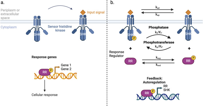 FIGURE 1
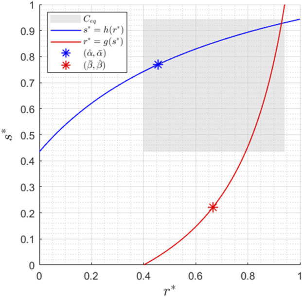 FIGURE 2
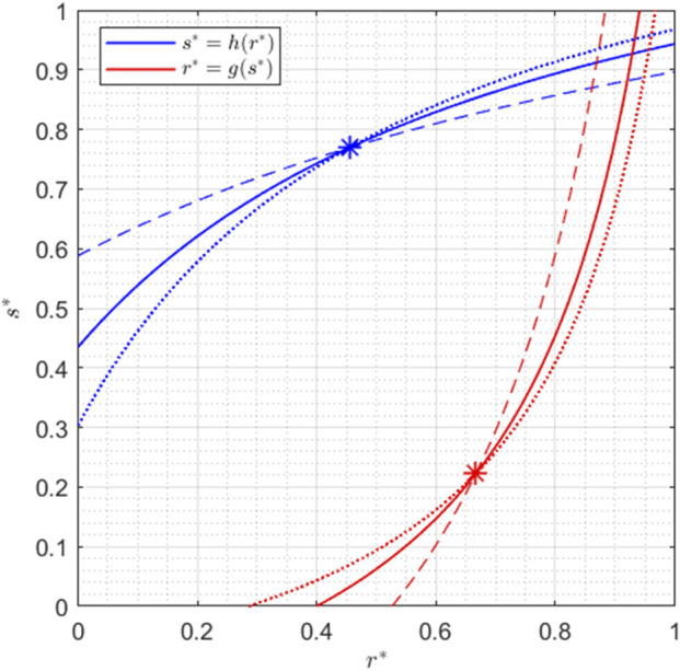 FIGURE 3
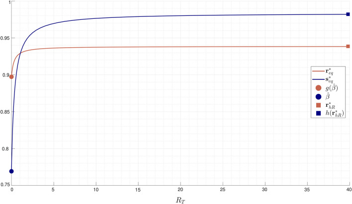 FIGURE 4
| References | Findings from previous studies | Model results of this study |
|---|---|---|
|
| Robustness of RR-P steady-state levels when SHK is limiting; EnvZ/OmpR experiments confirmed robustness to fluctuations in protein abundance. | Reproduces robustness when exogenous phosphorylation is absent. Predicts loss of robustness (steady state depends on SHK:RR ratio) if exogenous phosphorylation flux is present. |
|
| Formalized conditions for input–output robustness; robustness breaks down when multiple phosphorylation/dephosphorylation pathways exist. | General model confirms robustness only under restricted architectures. Multiple independent routes compromise robustness. |
| ( | Proposed and observed reverse phosphotransfer (RR-P | Extends framework to include reverse phosphotransfer. Predicts that it does not affect RR-P steady state (compensated by forward transfer), but increases phosphorylated SHK levels. |
Peer Reviews
No public reviews on file for this paper yet. If you reviewed it on a platform where reviews are public (OpenReview, ICLR, NeurIPS, ICML), you can paste yours below so the community can read it here.
Videos
No videos yet. Explain this paper in a talk, walkthrough, or lecture? Add one.
Taxonomy
TopicsBacterial Genetics and Biotechnology · Bacteriophages and microbial interactions · Protein Structure and Dynamics
1 Introduction
Bacteria rely on two-component systems (TCSs) as their primary signaling modules to detect environmental cues and orchestrate adaptive responses. A canonical TCS consists of a membrane-bound sensor histidine kinase (SHK) and a cytoplasmic response regulator (RR). Upon stimulation, the SHK autophosphorylates on a conserved histidine and transfers the phosphoryl group to an aspartate on the RR, generating the active form (RR-P) that typically regulates gene expression. This minimal architecture is remarkably versatile, underpinning processes such as chemotaxis, nutrient sensing, antibiotic resistance, and virulence regulation (Tierney and Rather, 2019; Tiwari et al., 2017; Kirby, 2009; Ramos et al., 2022; Alvarez and Georgellis, 2023).
Despite their apparent simplicity, TCSs display a rich spectrum of topologies and dynamic behaviors (Zschiedrich et al., 2016; Groisman, 2016; Stock et al., 2000). In some systems, exemplified by CheA in bacterial chemotaxis, SHK functions exclusively as a kinase, phosphorylating the RR. However, in many TCSs, SHK is bifunctional, participating in both phosphorylation and dephosphorylation of its cognate RR. In such cases, the input signal can modulate either one or both of these enzymatic activities, effectively tuning the rates of kinase and/or phosphatase reactions. TCSs may implement single-step phosphotransfers or multi-step phosphorelays, adding regulatory complexity and potentially delaying signal propagation.
At the transcriptional level, many TCSs feature autoregulation: the phosphorylated RR activates transcription of both its own gene and the gene encoding its partner SHK, thereby forming a positive feedback loop (Goulian, 2010). This feedback can alter steady-state behavior, activation, and inactivation kinetics and generate transient overshoot or “memory” effects, whereby the system responds faster to repeated stimuli. Although less common, negative autoregulation—or even mixed positive and negative feedback—has been observed in specific systems, providing an additional layer of response modulation. Auxiliary proteins can further diversify TCS behaviors, either by directly interacting with SHKs or RRs or by mediating cross-talk between otherwise independent TCS pathways (Rao et al., 2021; Groisman, 2016).
Mathematical modeling has been pivotal in elucidating the emergent properties of TCSs (summarized in Table 1). Batchelor and Goulian (2003) demonstrated that the steady-state level of RR-P can be robust to protein abundance fluctuations when SHK is limiting, a property supported by experimental data. Shinar et al. (2007) formalized the conditions for input-output robustness, showing that robustness is compromised when multiple independent phosphorylation or dephosphorylation routes exist. Igoshin et al. (2008) identified conditions for bistability, particularly when unphosphorylated SHK and RR form “dead-end” complexes or when alternative phosphatases modulate RR-P turnover. Ray and Igoshin (2010), Mitrophanov et al. (2010), and Zorzan et al. (2021) explored the role of transcriptional feedback, showing that autoregulation can alter response speed, overshoot amplitude, and even affect the effective sign of feedback, enabling TCSs to switch between positive and negative regulatory modes depending on signal strength. These studies collectively highlight how bifunctionality, phosphorelays, and feedback loops produce rich dynamic behaviors—including robustness, bistability, and adaptive memory—that are now central themes in systems-level analyses of TCSs.
In this study, we develop a systems-level model of a generalized TCS model focusing on the MprAB system from Mycobacterium tuberculosis that integrates canonical phosphorylation cycles, bifunctional enzymatic activity, transcriptional feedback, and potential auxiliary interactions. Our modeling framework seeks to (i) dissect how network architecture and parameter regimes shape dynamic properties and provide robustness, to be adopted as a building block to implement overshoots, oscillations, and bistability, and (ii) provide a predictive foundation for interpreting experimental dynamics and guiding synthetic circuit design in bacterial signal transduction.
By combining mechanistic modeling with systems-level analysis, this study elucidates how bifunctionality, phosphorelays, and feedback loops shape the dynamic behavior of TCSs, providing insights into bacterial adaptation and a framework for the rational engineering of synthetic signaling circuits (Mukherji and van Oudenaarden, 2009; Pasotti et al., 2017; Müller et al., 2025).
2 Two-component system: mathematical model
The model we consider is a general version of the model proposed in Tiwari et al. (2010) to describe the functioning of the two-component system MprA/MprB in M. tuberculosis in its active state.
For the sake of generality, we refer to “response regulator” and “sensor histidine kinase” rather than to MprA and MprB, respectively. Denoting by and , the concentration of (phosphorylated ) and (phosphorylated ), respectively, the dynamic evolution of the two-component system is described by the following set of ODEs (see Supplemental Information of Tiwari et al. (2010), Equations (S39)–(S42)):
—where
- and are the production rate constants of and , respectively;1
- is the rate constant for the -dependent dephosphorylation of ;
- is the Michaelis–Menten constant for dephosphorylation by ;
- is the rate constant for the -dependent phosphorylation of ;
- is the Michaelis–Menten constant for – phosphotransfer;
- and are the exogenous phosphorylation and dephosphorylation rate constants, respectively;
- and are the autophopshorylation and autodephosphorylation rate constants, respectively;
- is the protein degradation rate (assumed equal for and ).
One additional assumption worth highlighting is that the system is always considered to be in the active state. This is biologically reasonable as external stimuli often saturate the sensing capacity of the TCS. As a result, the transition of the sensor from the inactive to the active state upon binding external stimuli can be neglected in the model, as well as the availability of ATP inside the cell to provide phosphate groups for the phosphorylation steps.
The overall system can be represented as in Figure 1.
Schema of the generalized TCS. Binding of the signal molecule and general activation of genes are reported in panel (a), while in panel (b) the part of the system described by Equations 1–4 is reported.
We define the total amount of and as and , respectively, and rewrite the previous model presented in Equations 1–4 in the form shown in Equations 5–8:
—where is the net production rate of . Due to the separation of timescales between protein accumulation and phosphorylation/dephosphorylation events, we can assume that total concentrations of and are preserved—namely, that and are constant. Under this assumption, we can normalize all state variables and consider the phosphorylated portion of and
the dynamics of which are described by
Since we aim to provide a model describing the functioning of general two-component systems (TCSs) and unveiling its structural and asymptotic properties, from now on we will consider the following general formulation:
Differential Equations 9, 10 describe the dynamics of the phosphorylated portions of and —that is, ratio phosphorylated- (phosphorylated- ) over total —under the assumption that total concentrations and are constant. Notice that in Equation 10, the terms and have been included for reasons of symmetry. Of course, this general formulation can be tailored to the specific two-component system under investigation. For instance, we immediately verify that, upon defining
Equations 9, 10 reduce to the MprA-MprB system proposed in Tiwari et al. (2010).
2.1 Structural properties
We note that, by the way that has been defined, it is dimensionless, and such that for every it holds , means that all are unphosphorylated, while represents the situation with all phosphorylated. Clearly, the same holds for , and hence every state trajectory of the bidimensional system Equations 9, 10 belongs to the feasibility set .
Proposition 1 The TCS model Equations 9, 10 exhibits a unique equilibrium point within the feasibility set .
Proof. First, notice that the set is positively invariant with respect to systems Equations 9, 10, so that if the state trajectory starts in , then it stays in for any . Positive invariance of the convex and compact set ensures that there exists at least one equilibrium point in —that is, a limit cycle or at least one stable equilibrium point (Blanchini and Miani, 2015—Theorem 4.21).
We now resort to Bendixon’s theorem to rule out the existence of closed orbits.2 Note that
Hence, is not identically zero in any sub-region of the simply connected region and does not change sign in . Then, by Bendixon’s theorem (Sastry, 1999—Theorem 2.7), the set contains no closed orbits of system Equations 9, 10.
Finally, we resort to nullcline analysis to prove the uniqueness of steady states. Setting and yields the following expressions for and nullclines:
A typical figure of and nullclines is reported in Figure 2.
Nullclines for α1=0.5 , α2=1 , α3=1 , α4=7 , β1=0.3 , β2=1 , β3=1 , β4=4 , RT=1 , and ST=1 . The Ceq region corresponds to the subregion where the equilibrium point is located, as detailed in Proposition 2.
From expression 11, it is easy to obtain :
We define the function and note that, by the way has been defined, if is an equilibrium point, then ; vice versa, if then is an equilibrium point. It is a matter of computation to verify that is a rational function— —and that both the numerator and denominator are polynomials of order 2:
Note that for every , and hence for some if and only if for some . Since and , there certainly exists such that , and hence —as already demonstrated, the system admits at least one equilibrium point in . On the other hand, since is a second-order polynomial, such an belonging to the interval [0,1] is unique—the system admits a unique equilibrium point .
Remark 1Remark 1. A closed-form expression for the equilibrium point of the TCS can be computed as the unique root in interval [0,1] of the second-order polynomial .
with.
Proposition 1 states that all trajectories with initial conditions in converge to a unique equilibrium point . This means that, independently of the initial relative amounts of phosphorylated and unphosphorylated proteins, the proportion of phosphorylated to total will asymptotically equal , while the proportion of phosphorylated to total will asymptotically tend to . The following proposition identifies a subregion where the equilibrium point is located and hence provides upper and lower bounds to the phosphorylation levels and asymptotically reached by the TCS.
Proposition 2Consider the TCS described by models Equations 9, 10. The unique equilibrium point of the system, denoted by , belongs to the subregion
where
Proof. Consider the expression for nullcline Equation 11 and note that
and hence is strictly monotonically increasing in . The bounds on then follow from
Analogous computations on nullcline Equation 12 lead to upper and lower bounds on .
The set is reported in Figure 2 for the set of parameters considered. We conclude this section with the following Lemma, which will be useful for subsequent derivations (see again Figure 2).
Lemma 1 Consider the TCS described by models Equations 9, 10, and define
Then, nullcline Equation 11 always passes through — —while nullcline Equation 12 always passes through — .
This behavior can also be observed in Figure 3, where the dotted lines indicate the nullclines associated with higher values of and , while the dashed lines are the nullclines obtained with lower values of and , as described in the caption.
Nullclines for α1=0.5 , α2=1 , α3=1 , α4=7 , β1=0.3 , β2=1 , β3=1 , and β4=4 . The solid lines have RT=1 and ST=1 as in Figure 2; the dashed lines are obtained with RT=0.4 and ST=0.4 ; the dotted lines with RT=2 and ST=2 .
Since verifying that and is just a matter of computation, the proof of Lemma 1 is omitted.
At this point, two observations are in order. First, the dimensionless values and depend on the total amounts of and proteins present within the system (recall that, due to time scale separation, so far we have assumed that the quantities and are constant). In other words, and are continuous functions of and — and . The second observation is that uniform monotonicity of and with respect to their arguments is not guaranteed. Depending on the values taken by the system parameters, equilibrium might decrease with when belongs to a specific interval, and increase with when it belongs to a different interval.
3 Relative concentrations
3.1 Low vs high
RT concentration
In this section, we assume that and are independent.
Proposition 3 (Low concentration.) Consider the TCS described by models Equations 9, 10 and let the total concentration be arbitrary but fixed. When the total concentration is extremely low—that is, for —the equilibrium point asymptotically reached by the system is given by .
Proof. By taking the limit for of the function defined in Equation 12 and representing nullcline,3 it can be seen that . The result then follows by plugging into -nullcine Equation 11.
Proposition 4(High concentration.) Consider the TCS described by models Equations 9, 10 and let the total concentration be arbitrary but fixed. When the total concentration is extremely high—that is, for —the equilibrium point asymptotically reached by the system is , with being the (unique) solution in the interval [0,1] of the quadratic equation , where
More specifically, .
Proof. Note that when , the upper and lower bounds on are given by and , respectively, and hence do not provide any useful information. Taking the limit for of and nullclines Equations 13, 12 yields
Solving for leads to the quadratic equation . The result now follows upon noting that if , then and , otherwise ; by Descartes’ rule of signs, the quadratic equation has a unique positive solution.
Corollary 1 Consider the TCS described by models Equations 9, 10 and let the total concentration be arbitrary but fixed. Assuming the total concentration to be very high—that is, —then if and , the equilibrium point asymptotically reached by the system is ; if and , the equilibrium point is .
Proof. Consider the scenario with and and note that in this case, . Taking the limit for of nullcline (12) yields
Then, from nullcline Equation 11, we have 4. The proof for the case and follows the same line and is hence omitted.
Figure 4 reports, for an illustrative set of parameters, equilibrium values and as a function of .
Equilibrium values req and seq* continuously depend on the total amount of RR protein RT . Parameter values: α1=0.5 , α2=1 , α3=1 , α4=7 , β1=0.3 , β2=1 , β3=1 , β4=4 , and ST=1 .*
By symmetry, analogous results on the equilibrium point hold when the total amount is extremely low or extremely high— or .
3.2 Uniform monotonicity of the equilibrium with respect to
RT and ST
We now consider small perturbations of and concentrations and investigate their effects on the equilibrium point .
We assume first that is constant and consider small perturbations of . The equilibrium values continuously depend on —that is, —and this dependence is quantitatively described by
Conversely, if we assume that total concentration is constant while slowly varies, we have
Putting together Equations 14–17 and solving for the variation of equilibria with respect to and , we obtain
Proposition 5Consider the TCS described by model Equations 9, 10, and let denote the (unique) equilibrium point of the system. The equilibrium values and are:
- i) monotonically increasing in their arguments if and ;
- ii) monotonically decreasing in their arguments if and .
Proof. Observe that
and by symmetry, also for every . Moreover, recall that the function is such that and (see proof of Theorem 1), and hence at the equilibrium — . This, in turn, implies that
Then, the sign of the partial derivatives Equations 18, 19 are solely determined by and since all other terms are always non-negative. It is a matter of computation to verify that
and hence at equilibrium . Exploiting again the symmetry of the system, we can claim that . Hence, provided that is greater than (respectively, ), both and are monotonically increasing functions of (respectively, ). Similarly, provided that is smaller than (respectively, ), both and are monotonically decreasing functions of (respectively, ). It is clear from Figure 2 that when and , the equilibrium values necessarily satisfy the inequalities and , and the thesis follows.
Remark 2 The conditions on the system parameters provided by proposition 5 are sufficient (but not necessary) for uniform monotonicity of the equilibrium concerning total concentrations and . It is worth noticing that such a result is extremely powerful; its strength resides in the fact that it does not depend on the specific form of the functions and (provided they are monotone). More specifically, let and , where is an external signal and and are monotone functions. Then, , and the relationship between and is given by (note that the composite function is itself monotone). Proposition 5 states that if and , monotonicity of the equilibrium with respect to and is ensured independently on the specific form of the monotone functions and . If the previous conditions are not satisfied, uniform monotonicity is not guaranteed.
We now focus on the case where a proportionality relationship among and can be assumed: . Note that this is a perfectly reasonable assumption when phosphorylated activates the transcription of both its gene and the gene encoding its partner —see, for example, the mathematical description of the MprA/MprB two-component system adopted in (Tiwari et al., 2010).
Theorem 1 Consider the TCS described by models Equations 9, 10 , and assume that total and concentrations are related by , where is a fixed (not necessarily known) proportionality coefficient. When the total concentration is extremely high—that is, for —the (unique) equilibrium point asymptotically reached by the system is
Proof. Compute the limit for of and nullclines Equations 11, 12:
From expression Equation 21, it is easy to obtain
Substituting the previous expression into Equation 20 and solving for yields the following quadratic equation:
Then, the only two possible equilibrium points are and . To determine which is the right solution, we need to resort to the intersection condition (see the proof of Proposition 5). Indeed, it is straightforward to verify that
and hence
which uniquely determines the limiting equilibrium pair once the quantity is known.
Remark 3 The previous result does not require knowledge of the value assumed by the proportionality coefficient ; we just need to know that a proportionality coefficient continuously relates and
4 Absolute concentrations
We have thus far analyzed the properties (asymptotic behavior and monotonicity) of relative concentrations: of the ratio between phosphorylated and unphosphorylated protein concentrations. A fundamental and crucial point is that these properties do not necessarily hold for absolute concentrations too: the fact that the relative concentration tending to 0 does not imply that absolute concentration tends to 0; similarly, uniform monotonicity of for does not imply uniform monotonicity of to . To understand this point, note that the relative concentration tends to 0 when total concentration asymptotically grows to infinity (i.e., ) and asymptotically approaches a given saturation level . Regarding monotonicity, since , it holds that
It is clear that if is a monotonically increasing function of (namely, ), so is . On the contrary, if is a monotonically decreasing function of , and hence ; monotonicity of with respect to is not guaranteed.
In the following, we analyze the asymptotic behavior of absolute concentrations and when grows to infinity, under the assumption that and total concentrations are linearly related with the proportionality coefficient — .
Theorem 2 Consider the TCS described by models Equations 9, 10 and assume that the total and concentrations are linearly related by , where is a fixed proportionality coefficient. When total concentration is sufficiently high—that is, for , and —then absolute concentrations asymptotically approach the equilibrium values:
respectively.
Proof. We claim that for a sufficiently high , absolute equilibrium concentrations and asymptotically approach saturation levels and :
We now seek to determine the values and . First, we note that
Analogously, the limit of for can be computed as
Therefore, we need to solve the linear system:
Solving for and yields
Thus, the proof is concluded.
It follows from Theorem 2 that for sufficiently high , while the amount of phosphorylated increases with , the amount of phosphorylated is a decreasing function of , such that
5 Discussion
A distinguishing feature of the proposed TCS mathematical model is that it accounts for a variety of reactions, including phosphorylation and dephosphorylation through external (exogenous) pathways, autophosphorylation and autodephosphorylation, phosphorylation via phosphotransfer from , and dephosphorylation via . Of course, by setting 0 for one or more parameters, the model can be tailored to specific two-component systems (TCSs) and/or situations in which some of the previous reactions are negligible.
One of the best characterized examples of TCS is the EnvZ/OmpR system in Escherichia coli, which responds to changes in environmental osmolality by regulating the expression of the outer membrane porins OmpF and OmpC. As in many TCSs, EnvZ is a bifunctional sensor histidine kinase, meaning that it phosphorylates and dephosphorylates the response regulator OmpR. Batchelor and Goulian (2003) proposed a mathematical model of the EnvZ/OmpR TCS and experimentally tested the model’s predictions. Their main finding was that for sufficiently high amounts of OmpR, when total EnvZ in the cell is much less abundant than total OmpR 5, the steady-state level of phosphorylated OmpR is robust (insensitive) to fluctuations in EnvZ and OmpR concentrations. This model accounts for the autokinase, phosphotransfer, and phosphatase activities of EnvZ and neglects the exogenous phosphorylation and dephosphorylation of OmpR. Casting such a scenario into our mathematical framework means setting and to 0. Theorem 2 then implies that the equilibrium absolute concentration for OmpR is given by , and hence, consistent with Batchelor and Goulian (2003), does not depend on EnvZ total concentration. However, our model shows that if an exogenous phosphorylation flux is present ( ), the previous result fails; when an external pathway for OmpR phosphorylation is present, the steady-state concentration of phosphorylated OmpR is (higher and) decreasing with (see Equation 22). Notably, Batchelor and Goulian (2003) predicted, via theoretical analysis and experimental verification with fluorescent reporter strains, that when condition does not hold, the steady-state value of OmpR-P decreases with increasing total EnvZ concentration. This is consistent with our theoretical results, which also shed light on the role of an EnvZ-independent mechanism for OmpR phosphorylation.
Furthermore, our analysis allows the characterization of the steady-state concentration of the histidine kinase: (recall that ). As expected, our model predicts that the amount of phosphorylated EnvZ increases with more vigorous autokinase activity and decreases with stronger phosphotransfer activity of the histidine kinase .
Finally, while our analysis demonstrates the existence of a single robust equilibrium of the system (Theorem 1), it is instructive to consider the possibility of using such a building block as part of a closed-loop system with positive retroactivity, which could lead to oscillatory or bistable behaviors (Igoshin et al., 2008; Zorzan et al., 2021; Tiwari et al., 2010).
5.1 Phosphotransfer and reverse phosphotransfer reactions
Bifunctional sensor histidine kinase exerts both positive and negative control through phosphotransfer and phosphatase activity, respectively. While the biochemical reactions underlying kinase activity are reasonably well understood, the mechanisms of phosphatase activity represent a long-standing question, the investigation of which has led to the formulation of multiple hypotheses (see Huynh and Stewart, 2011 for an overview). An early hypothesis, first proposed by Dutta and Inouye (1996), identified reverse transfer of the phosphoryl group from phosphorylated to as a potential dephosphorylation mechanism. Such a hypothesis was prompted by experimental results conducted on EnvZ/OmpR system in E. coli (Dutta and Inouye, 1996; Zhu et al., 2000), showing that reverse transfer of the phosphoryl group from OmpR-P to EnvZ was detected in the early period of the phosphatase reaction with domain A of EnvZ—specifically with the EnvZ mutant (EnvZ.N347D), and, under certain conditions, with the wild-type EnvZ.
Even if later experiments invalidated the reverse phosphotransfer model (Hsing and Silhavy, 1997), it is universally recognized that reverse phosphotransfer can occur under certain conditions. As pointed out by Gao and Stock (2009), multiple mechanisms may have evolved for phosphatase activities, and individual histidine kinases may utilize different regulatory strategies. We now aim to theoretically investigate a scenario in which both direct and reverse phosphotransfer reactions occur, and a distinct phosphatase activity of the sensor histidine is present.
Since the kinase activity of takes the form of a phosphotransfer reaction (by which a phosphoryl group is transferred from phosphorylated to ), reaction rates and are actually equal— . We first assume that only exhibits phosphotransfer activity ( ), and we rename as , where superscript stands for “phosphatase activity” (of the ). It follows from Theorem 2 that when total concentration is sufficiently high, steady-state absolute concentrations are given by and .
When reverse phosphotransfer from phosphorylated to occurs, the reaction rate is non-zero and , with (where superscript stands for “reverse phosphotransfer”). Then, recalling that , Theorem 2 yields
This indicates that, even if reverse phosphotransfer occurs, the absolute concentration of phosphorylated remains unchanged. While this may seem contradictory at first, it is easily explained by noting that reverse phosphotransfer from phosphorylated to is exactly compensated by the increased direct phosphotransfer from phosphorylated to . On the contrary, when the reverse phosphotransfer reaction occurs, our analysis shows that the absolute concentration of increases and that such an increase is larger for higher values of the reverse phosphotransfer rate (bigger ) and/or for larger amounts of total concentration (bigger ).
This study’s main findings are summarized here in comparison with the literature.
6 Conclusion
We here developed a generalized mathematical model for bacterial two-component signaling systems that integrates canonical phosphorylation cycles, bifunctional enzymatic activities, transcriptional feedback, and potential auxiliary interactions. Through systems-level analysis, we elucidated how network architecture and parameter regimes shape key dynamic properties and robustness.
Our modeling framework provides a predictive foundation for interpreting experimental dynamics, as illustrated for the EnvZ/OmpR system, and for guiding the rational design of synthetic signaling circuits. We demonstrated that the bifunctionality of the sensor histidine kinase, multi-step phosphorelays, and transcriptional feedback, which are incorporated into the model, enable rich behaviors that allow TCSs to precisely tune cellular responses to diverse environmental stimuli.
Notably, we derived analytical conditions in Propositions 3, Propositions 4, Propositions 5 and Theorem 1 under which the steady-state levels of phosphorylated proteins exhibit input–output robustness, overshoot, or bistability. We also characterized in Sections 3–4 how the equilibrium phosphorylation levels depend on the absolute and relative abundances of the two components. These insights are critical for understanding natural mechanisms of bacterial adaptation and for forward-engineering synthetic gene circuits with prescribed dynamics.
By combining the mechanistic modeling framework with systems analysis techniques, such as nullcline analysis, this study provides a unified perspective on the structural design principles that underlie the remarkable versatility of two-component signal transduction. The proposed generalized model lays a theoretical foundation for further experimental investigations, such as exploring reverse phosphotransfer mechanisms, and establishes a framework for rationally harnessing two-component systems in synthetic biology applications.
The reference list from the paper itself. Each links out to its DOI / PubMed record.
- 1Alvarez A. F.Georgellis D. (2023). Environmental adaptation and diversification of bacterial two-component systems. Curr. Opin. Microbiol. 76, 102399. 10.1016/j.mib.2023.102399 39399893 · doi ↗ · pubmed ↗
- 2Batchelor E.Goulian M. (2003). “Robustness and the cycle of phosphorylation and dephosphorylation in a two-component regulatory system,”, 100. Proceedings of the National Academy of Sciences, (Washington, D.C., USA: National Academy of Sciences), 691–696. 10.1073/pnas.0234782100 PMC 14105812522261 · doi ↗ · pubmed ↗
- 3Blanchini F.Miani S. (2015). Set-theoretic methods in control systems and control: Foundations and applications. Basel, Switzerland: Birkhäuser Basel.
- 4Dutta R.Inouye M. (1996). Reverse phosphotransfer from Omp R to Env Z in a kinase-/phosphatase+ mutant of Env Z (Env Z.N 347D), a bifunctional signal transducer of Escherichia coli . J. Biol. Chem. 271, 1424–1429. 10.1074/jbc.271.3.1424 8576133 · doi ↗ · pubmed ↗
- 5Gao R.Stock A. (2009). Biological insights from structures of two-component proteins. Annu. Rev. Microbiol. 63, 133–154. 10.1146/annurev.micro.091208.073214 19575571 PMC 3645274 · doi ↗ · pubmed ↗
- 6Goulian M. (2010). Two-component signaling circuit structure and properties. Curr. Opin. Microbiol. 13, 184–189. 10.1016/j.mib.2010.01.009 20149717 PMC 2847654 · doi ↗ · pubmed ↗
- 7Groisman E. (2016). Feedback control of two-component regulatory systems. Annu. Rev. Microbiol. 70, 103–124. 10.1146/annurev-micro-102215-095331 27607549 PMC 8380452 · doi ↗ · pubmed ↗
- 8Hsing W.Silhavy T. (1997). Function of conserved histidine-243 in phosphatase activity of Env Z, the sensor for porin osmoregulation in Escherichia coli . J. Bacteriol. 179, 3729–3735. 10.1128/jb.179.11.3729-3735.1997 9171423 PMC 179171 · doi ↗ · pubmed ↗