Study on coal and gas outburst prediction technology based on multi-model fusion
Qian Xie, Junsheng Yan, Zhenhua Dai, Wengang Du, Xuefei Wu

TL;DR
This study introduces a new AI-based framework that combines multiple machine learning models to improve predictions of coal and gas outbursts in mines.
Contribution
A novel multi-model fusion framework using ensemble learning and model Stacking for coal and gas outburst prediction is proposed.
Findings
The ensemble model outperforms single-model approaches in predicting coal and gas outbursts.
The proposed framework achieves a higher F1-score, indicating improved prediction accuracy.
Base learners like SVM, RF, and KNN contribute complementary strengths when combined.
Abstract
The rapid advancement of artificial intelligence (AI) and machine learning (ML) technologies has opened up novel avenues for predicting coal and gas outbursts in coal mines. This study proposes a novel prediction framework that integrates advanced AI methodologies through a multi-model fusion strategy based on ensemble learning and model Stacking. The proposed model leverages the diverse data interpretation capabilities and distinct training mechanisms of various algorithms, thereby capitalizing on the complementary strengths of each constituent learner. Specifically, a Stacking-based ensemble model is constructed, incorporating Support Vector Machines (SVM), Random Forests (RF), and k-Nearest Neighbors (KNN) as base learners. An attention mechanism is then employed to adaptively weight the outputs of these base learners, thereby harnessing their complementary strengths. The…
Click any figure to enlarge with its caption.
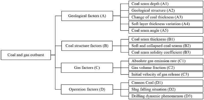 Figure 1
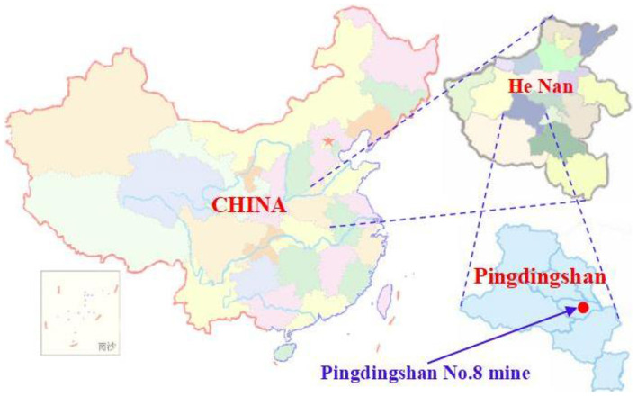 Figure 2
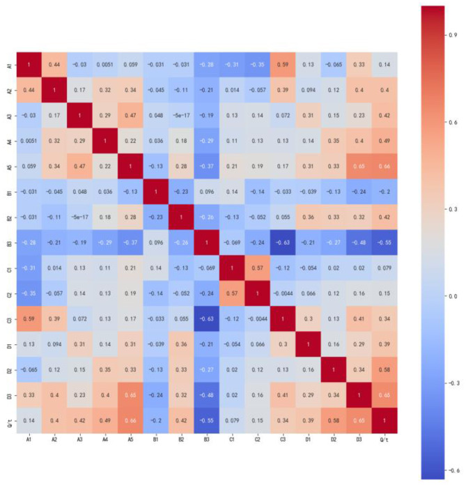 Figure 3
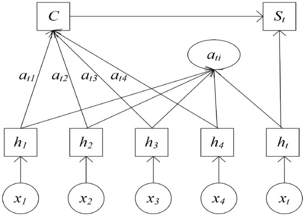 Figure 4
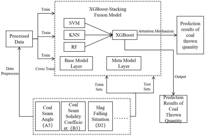 Figure 5
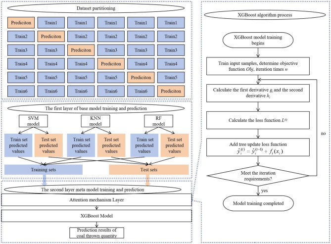 Figure 6
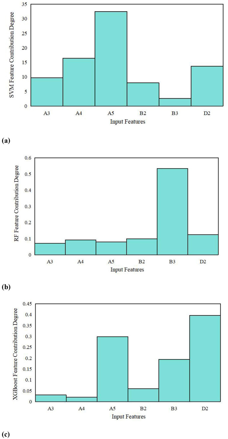 Figure 7
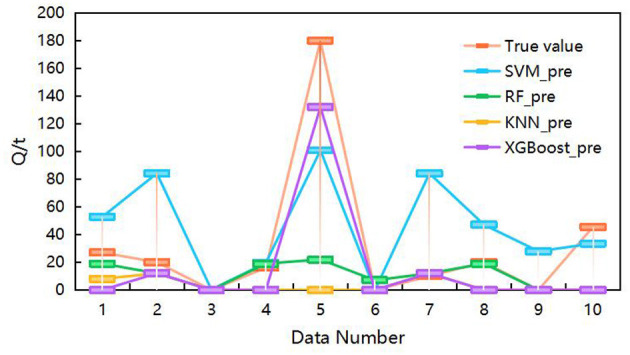 Figure 8
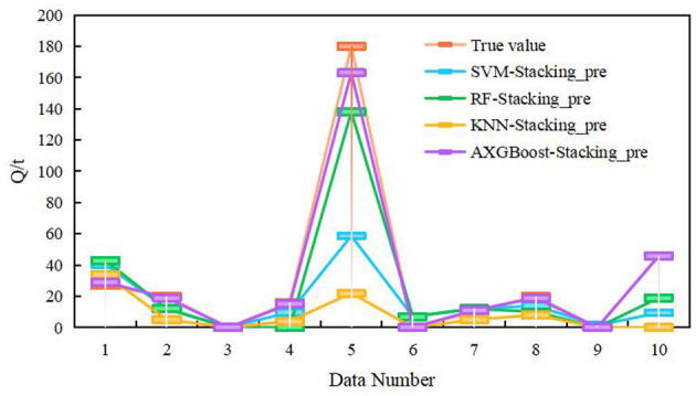 Figure 9
|
|
|
|
|---|---|---|
| I | No outburst | 0 |
| II | Small outburst | 0 < |
| III | Medium outburst | 50 < |
| IV | Large outburst | 100 < |
| V | Extra-large outburst | 500 < |
|
|
|
|
|
|
|
|
|
|
|
|
|
|
|
|
|
|
|---|---|---|---|---|---|---|---|---|---|---|---|---|---|---|---|---|
| 1 | 535 | 3 | 3 | 1 | 1 | 5.4 | 1 | 0.32 | 0.66 | 0.4 | 11.23 | 3 | 1 | 1 | 19.7 | II |
| 2 | 522 | 3 | 1 | 3 | 1 | 4.8 | 1 | 0.35 | 1.93 | 0.5 | 10.17 | 1 | 3 | 1 | 16 | II |
| 3 | 584 | 3 | 1 | 1 | 5 | 3.2 | 3 | 0.2 | 2.38 | 0.53 | 12.06 | 3 | 1 | 5 | 132 | IV |
| 4 | 484 | 3 | 3 | 1 | 3 | 4.81 | 1 | 0.53 | 5.25 | 0.5 | 4.75 | 1 | 1 | 1 | 12 | II |
| 5 | 566 | 5 | 1 | 1 | 1 | 3.5 | 1 | 0.51 | 0.36 | 0.2 | 9 | 1 | 1 | 1 | 30 | II |
| 6 | 463 | 1 | 1 | 3 | 1 | 4.81 | 3 | 0.26 | 6.24 | 0.6 | 4.8 | 3 | 3 | 1 | 46 | II |
| 7 | 490 | 3 | 1 | 1 | 1 | 4.81 | 1 | 0.49 | 6.24 | 0.6 | 7.81 | 3 | 1 | 1 | 28 | II |
| 8 | 424 | 1 | 1 | 1 | 1 | 3.65 | 3 | 0.51 | 0.47 | 0.27 | 8.53 | 3 | 1 | 1 | 6 | II |
| 9 | 535 | 3 | 1 | 1 | 1 | 5.2 | 3 | 0.29 | 3.68 | 0.49 | 17.14 | 3 | 1 | 1 | 62 | III |
| 10 | 566 | 5 | 3 | 3 | 3 | 3.5 | 1 | 0.38 | 1.04 | 0.75 | 8.57 | 3 | 3 | 3 | 144.6 | IV |
| 11 | 563.4 | 5 | 1 | 1 | 1 | 3.7 | 1 | 0.57 | 0.76 | 0.4 | 8.76 | 1 | 1 | 3 | 53 | II |
| 12 | 564 | 5 | 1 | 1 | 1 | 3.7 | 1 | 0.57 | 0.7 | 0.38 | 7.24 | 1 | 1 | 1 | 0 | I |
| 13 | 485 | 5 | 3 | 5 | 3 | 3.3 | 1 | 0.11 | 7.8 | 1.2 | 19.65 | 3 | 3 | 5 | 450 | IV |
| 14 | 482 | 3 | 1 | 1 | 1 | 3.4 | 1 | 0.14 | 7.6 | 1.3 | 18.64 | 1 | 1 | 1 | 0 | I |
| 15 | 623 | 3 | 3 | 1 | 3 | 4.5 | 1 | 0.35 | 0.44 | 0.3 | 14.27 | 3 | 1 | 1 | 22 | II |
| 16 | 584 | 3 | 1 | 1 | 3 | 3.2 | 1 | 0.24 | 2.32 | 0.5 | 11.86 | 1 | 1 | 3 | 0 | I |
| 17 | 557.6 | 1 | 1 | 1 | 1 | 3.1 | 3 | 0.54 | 0.52 | 0.4 | 11.38 | 3 | 3 | 1 | 43 | II |
| 18 | 557.6 | 1 | 3 | 1 | 1 | 3.4 | 3 | 0.15 | 0.78 | 0.6 | 18.85 | 3 | 3 | 3 | 240 | IV |
| 19 | 557.6 | 1 | 1 | 1 | 1 | 3.2 | 3 | 0.46 | 0.36 | 0.5 | 9.48 | 1 | 1 | 1 | 0 | I |
| 20 | 486 | 1 | 1 | 1 | 1 | 3.5 | 3 | 0.29 | 0.33 | 0.38 | 12.56 | 3 | 1 | 1 | 22 | II |
| 21 | 529.8 | 3 | 1 | 3 | 1 | 4.3 | 3 | 0.67 | 0.42 | 0.32 | 11.48 | 3 | 3 | 1 | 5 | II |
| 22 | 583 | 1 | 1 | 1 | 1 | 4.5 | 3 | 0.43 | 1.15 | 0.7 | 9.18 | 3 | 3 | 3 | 10 | II |
| 23 | 583 | 1 | 1 | 1 | 1 | 4.7 | 1 | 0.46 | 1.05 | 0.66 | 9.24 | 1 | 1 | 1 | 0 | I |
| 24 | 533 | 5 | 3 | 3 | 3 | 4.1 | 3 | 0.23 | 0.34 | 0.2 | 12.57 | 5 | 3 | 3 | 440 | IV |
| 25 | 530 | 5 | 1 | 1 | 1 | 4.1 | 1 | 0.36 | 0.32 | 0.18 | 12.38 | 1 | 3 | 1 | 0 | I |
| 26 | 622 | 3 | 1 | 1 | 1 | 3 | 1 | 0.32 | 2.31 | 0.5 | 20.19 | 3 | 1 | 1 | 64 | III |
| 27 | 573 | 1 | 1 | 1 | 1 | 4.1 | 3 | 0.5 | 0.79 | 0.34 | 7.33 | 3 | 1 | 1 | 16 | II |
| 28 | 537.9 | 3 | 1 | 1 | 3 | 5.3 | 1 | 0.19 | 0.22 | 0.8 | 23.91 | 3 | 3 | 3 | 138 | IV |
| 29 | 562 | 3 | 1 | 1 | 1 | 5.25 | 1 | 0.47 | 4.5 | 0.5 | 14.28 | 1 | 3 | 1 | 12.5 | II |
| 30 | 540 | 1 | 1 | 1 | 1 | 4.8 | 1 | 0.31 | 0.62 | 0.32 | 12.33 | 1 | 1 | 1 | 0 | I |
| 31 | 540 | 1 | 1 | 3 | 1 | 4.8 | 3 | 0.27 | 0.52 | 0.3 | 12.05 | 1 | 1 | 1 | 8 | II |
| 32 | 457 | 1 | 1 | 1 | 3 | 3.5 | 3 | 0.15 | 1.95 | 0.6 | 5.09 | 1 | 5 | 1 | 478 | IV |
| 33 | 460 | 1 | 1 | 1 | 1 | 3.5 | 1 | 0.38 | 1.38 | 0.52 | 4.68 | 1 | 1 | 1 | 0 | I |
| 34 | 589 | 3 | 1 | 1 | 1 | 3.2 | 3 | 0.24 | 2.1 | 0.6 | 11.05 | 1 | 1 | 1 | 4.6 | II |
| 35 | 636.4 | 5 | 3 | 3 | 5 | 3.2 | 3 | 0.15 | 3.08 | 0.46 | 18.25 | 3 | 5 | 5 | 396 | IV |
| 36 | 584 | 3 | 1 | 1 | 5 | 3.2 | 3 | 0.25 | 2.94 | 0.7 | 14.18 | 5 | 3 | 5 | 215 | IV |
| 37 | 564.6 | 5 | 1 | 1 | 1 | 3.5 | 1 | 0.48 | 0.78 | 0.6 | 9.27 | 3 | 1 | 1 | 44 | II |
| 38 | 480 | 1 | 1 | 1 | 1 | 4.81 | 1 | 0.53 | 5.25 | 0.5 | 4.75 | 1 | 1 | 1 | 0 | I |
| 39 | 840 | 7 | 3 | 3 | 5 | 4.5 | 3 | 0.17 | 1.15 | 0.25 | 23.52 | 3 | 3 | 5 | 551 | IV |
| 40 | 838 | 5 | 1 | 1 | 1 | 4.5 | 1 | 0.26 | 1.03 | 0.25 | 20.86 | 1 | 1 | 3 | 0 | I |
| 41 | 566 | 5 | 1 | 3 | 1 | 3.5 | 1 | 0.51 | 0.48 | 0.6 | 7.93 | 1 | 1 | 1 | 55 | III |
| 42 | 620 | 1 | 1 | 1 | 1 | 3 | 1 | 0.34 | 1.83 | 0.46 | 18.75 | 1 | 1 | 1 | 0 | I |
| 43 | 800 | 5 | 1 | 3 | 1 | 3.3 | 3 | 0.18 | 0.42 | 0.22 | 15.89 | 1 | 3 | 5 | 190 | IV |
| 44 | 820 | 5 | 1 | 1 | 1 | 4.5 | 1 | 0.21 | 1.22 | 0.28 | 20.31 | 1 | 1 | 1 | 0 | I |
| 45 | 614 | 1 | 1 | 1 | 1 | 4.5 | 1 | 0.55 | 5.4 | 0.3 | 9.87 | 3 | 1 | 1 | 7 | II |
| 46 | 697 | 1 | 1 | 1 | 1 | 4.1 | 1 | 0.35 | 0.58 | 0.12 | 15.91 | 3 | 1 | 1 | 14 | II |
| 47 | 629 | 3 | 1 | 1 | 1 | 4.5 | 1 | 0.34 | 0.99 | 0.18 | 15.67 | 1 | 1 | 3 | 32 | II |
| 48 | 490 | 3 | 1 | 1 | 1 | 3.2 | 1 | 0.51 | 0.85 | 0.15 | 14.32 | 1 | 5 | 1 | 34 | II |
| 49 | 652 | 1 | 1 | 1 | 1 | 4 | 1 | 0.54 | 0.5 | 0.52 | 12.03 | 3 | 1 | 3 | 5 | II |
| 50 | 820 | 7 | 1 | 1 | 1 | 4.5 | 1 | 0.19 | 1.22 | 0.3 | 24.71 | 5 | 1 | 1 | 115 | IV |
| 51 | 554 | 1 | 3 | 3 | 1 | 5.4 | 1 | 0.28 | 0.35 | 0.3 | 15.47 | 3 | 1 | 1 | 27 | II |
| 52 | 482 | 3 | 3 | 1 | 3 | 4.81 | 1 | 0.53 | 6.24 | 0.6 | 4.75 | 1 | 1 | 1 | 20 | II |
| 53 | 550 | 1 | 1 | 1 | 1 | 5.4 | 1 | 0.4 | 0.28 | 0.25 | 10.48 | 1 | 1 | 1 | 0 | I |
| 54 | 606 | 1 | 3 | 1 | 1 | 2 | 1 | 0.41 | 0.34 | 0.45 | 7.99 | 3 | 1 | 1 | 16 | II |
| 55 | 557.6 | 3 | 3 | 1 | 3 | 3 | 3 | 0.24 | 1.5 | 0.5 | 21.06 | 3 | 1 | 3 | 180 | IV |
| 56 | 563 | 1 | 1 | 1 | 1 | 3.5 | 1 | 0.55 | 0.42 | 0.35 | 6.21 | 1 | 1 | 1 | 0 | I |
| 57 | 487 | 3 | 3 | 1 | 3 | 4.81 | 1 | 0.53 | 5.25 | 0.5 | 4.75 | 1 | 1 | 1 | 10 | II |
| 58 | 583 | 1 | 3 | 1 | 1 | 4.8 | 1 | 0.34 | 1.24 | 0.75 | 10.34 | 3 | 3 | 1 | 20 | II |
| 59 | 580 | 1 | 1 | 1 | 1 | 3.4 | 1 | 0.26 | 2.7 | 0.52 | 12.27 | 1 | 3 | 1 | 0 | I |
| 60 | 520 | 3 | 1 | 3 | 1 | 4.5 | 1 | 0.26 | 1.38 | 0.4 | 12.74 | 1 | 1 | 3 | 45.5 | II |
|
|
|
|
|---|---|---|
| Strong correlation | (0.6,0.8] | A5 and B3 |
| Moderately correlation | (0.4,0.6] | D2, A4, B2, and A3 |
| Weak correlation | (0/2,0.4] | A2, D1, and C3 |
| No correlation | (0,0.2] | C2, A1, C1, B1, and D3 |
|
|
|---|
| 1. Def attention_3d_block |
|
|
|
|
|
|
|---|---|---|---|---|
| SVM | Kernel = “linear”, | 1,821.56 | 13.16 | 0.875 |
| RF | n_estimators = 100, random_state = 0, n_jobs = −1 | 2,722.525 | 20.85 | 0.857 |
| KNN | n_neighbors = 3 | 3,555.525 | 28.65 | 0.6 |
| XGBoost | n_neighbors = 6, learining_rate = 0.09 | 582.725 | 16.25 | 0.6 |
|
|
|
|
|
|
|
| ||||
|---|---|---|---|---|---|---|---|---|---|---|
|
|
|
|
|
|
|
|
| |||
| 1 | 27 | II | 40.4188 | II | 43 | II | 34 | II | 29 | II |
| 2 | 20 | II | 12.0889 | II | 12 | II | 5 | II | 19 | II |
| 3 | 0 | I | 0.095 | I | 0 | I | 0 | I | 0 | I |
| 4 | 16 | II | 9.6556 | II | 0 | I | 4 | II | 15 | II |
| 5 | 180 | IV | 58.6095 | IV | 138 | IV | 22 | II | 163 | IV |
| 6 | 0 | I | 7.0851 | II | 7 | II | 0 | I | 0 | I |
| 7 | 10 | II | 12.0889 | II | 12 | II | 5 | II | 11 | II |
| 8 | 20 | II | 13.8117 | II | 10 | II | 8 | II | 19 | II |
| 9 | 0 | I | 1.3268 | II | 0 | I | 0 | I | 0 | I |
| 10 | 45.5 | II | 9.4444 | II | 19 | II | 0 | I | 46 | II |
|
|
|
|
|
|---|---|---|---|
| SVM-Stacking | 1,641.318 | 15.38 | 0.823 |
| RF-Stacking | 319.525 | 7.75 | 0.857 |
| KNN-Stacking | 2,762.125 | 24.05 | 0.923 |
| AXGBoost-Stacking | 29.725 | 1.65 | 0.98 |
- —Key Research and Development Projects of Shaanxi Province10.13039/501100015401
Peer Reviews
No public reviews on file for this paper yet. If you reviewed it on a platform where reviews are public (OpenReview, ICLR, NeurIPS, ICML), you can paste yours below so the community can read it here.
Videos
No videos yet. Explain this paper in a talk, walkthrough, or lecture? Add one.
Taxonomy
TopicsCoal Properties and Utilization · Geoscience and Mining Technology · Safety and Risk Management
1 Introduction
Coal and gas outbursts remain a significant threat to the safety of coal mine workers in China. In geologically complex regions, the deepening of mining activities further aggravates subsurface conditions, increasing both the frequency and severity of outburst-related incidents (Ou et al., 2023; Fu et al., 2022). Therefore, the development of accurate and reliable predictive models for coal and gas outbursts is critically important.
Extensive research has been conducted on predictive models for coal and gas outbursts, resulting in the development of a variety of approaches. These include the initial velocity method for borehole outbursts (Wang et al., 2020a), the drilling cuttings index method (Wang et al., 2020b), mathematical evaluation models (Soleimani et al., 2023; Hassan et al., 2017; Zhou et al., 2019; Rudakov and Sobolev, 2019; Yang et al., 2023), and AI-based models (Qiao et al., 2019; Anani et al., 2024; Li et al., 2024; Zhu et al., 2023; Song et al., 2021; Wang et al., 2023), all of which have demonstrated varying degrees of effectiveness. The rapid progress in AI technology has provided new opportunities for enhancing prediction accuracy. For instance, Fan et al. improved the SVM model using the firefly algorithm (FA) to predict coal and gas outbursts and validated its overall performance (Fan et al., 2023). Liu et al. used a least squares SVM optimized with the particle swarm optimization (PSO) algorithm, confirming its effectiveness using gas outburst data from the Jiulishan Coal Mine in Jiaozuo City, China (Liu et al., 2021). Furthermore, Zheng et al. (2023) used XGBoost to predict and analyze the contribution rate distribution of coal and gas outburst indicators. However, these aforementioned studies tend to treat coal and gas outburst prediction as an isolated task. Given the inherent uncertainties and complex underlying mechanisms of such predictions, multiple hypotheses may perform well on the training set. Relying on a single model may suffer from poor generalization due to its susceptibility to randomness and overfitting. To address these limitations, we proposed a novel multi-model fusion prediction method that integrates an attention mechanism for analyzing the contribution rates of coal and gas data (Zhao et al., 2024a; Lin et al., 2020). Initially, Pearson's correlation analysis was conducted to identify and select strongly correlated features as model inputs. Subsequently, within the Stacking ensemble framework, a coal and gas outburst prediction model that integrates multiple learners was constructed to capture a more comprehensive data observation space. Finally, the efficacy of the proposed model was rigorously validated using real-world data from the Pingdingshan Coal Mine in China. The results unequivocally demonstrate that the Stacking-based ensemble method with multi-model fusion achieves robust predictive performance for coal and gas outburst events.
2 Data analysis
2.1 Research overview and data sources
Coal and gas outbursts are influenced by four main factors: geological conditions, coal seam characteristics, gas-related factors, and operational practices. Based on field observations, these factors are further subdivided into 14 specific elements (He et al., 2010) (Figure 1). The risk level (L) of coal and gas outbursts is classified into five categories based on the amount of ejected coal (Table 1).
Factors influencing coal and gas outbursts.
In this study, we used coal and gas outburst data collected from a coal mine in Pingdingshan over a period spanning from 1984 to 2009 (Xie et al., 2018). The first 50 data points were selected as the training set, while the final 10 data points were reserved for testing purposes. The coal and gas outburst data from the Pingdingshan Coal Mine are summarized in Table 2. The geographical location of Pingdingshan is shown in Figure 2.
Geographical location of the No. 8 mine in Pingdingshan, China.
2.2 Data process
Before feeding the training data into the model, it is crucial to carefully preprocess the dataset by identifying and addressing any anomalies.
Step 1: The Pauta criterion was applied to establish the outlier threshold. Data points that deviated from the mean by more than three standard deviations were considered outliers. These outliers were then removed, and their corresponding entries were set to null values.
Step 2: Missing values were then filled by extracting the five data points preceding and following each missing entry. In this study, Lagrange interpolation was used to estimate the missing data, as shown in Equations 1, 2.
where li(x) represents the interpolation basis function; Ln(x) denotes the interpolated value of the missing data; yi is a known (non-missing) value; x is the index corresponding to the missing value; xi denotes the index of the known data point; and xj is the interpolation node.
2.3 Correlation analysis
The primary indicator for determining the severity of a coal and gas outburst was the quantity of coal thrown (Table 1). As shown in Figure 3, Pearson's correlation analysis was performed to rigorously investigate both the interrelationships among the various influencing factors and their individual correlations with the quantity of coal thrown, as defined by Equation 3.
where cov(X, Y) is covariance and σ_X_ and σY are the standard deviations of X and Y, respectively.
Pearson's correlation analysis of factors affecting coal and gas outbursts.
Following the strong and weak correlation partitions established by Zhang et al. (2022), the correlation results presented in Figure 3 were subsequently classified. The outcomes of this classification are comprehensively detailed in Table 3. As demonstrated in Table 3, this study meticulously selected six factors exhibiting medium to high correlation levels as input variables for the model, specifically including A5, B3, D2, A4, B2, and A3.
3 Methods
3.1 XGBoost principle
XGBoost is a prominent and highly efficient boosting ensemble learning algorithm, representing an advanced evolution of the Gradient Boosted Decision Tree (GBDT) model (Yao et al., 2022; Xiong et al., 2024; Utkarsh, 2024). The predictive output of the XGBoost model is formulated as shown in Equation 4:
where ŷ_i_ denotes the predicted value for the i-th sample; K represents the number of trees; F signifies the function space of the tree; xi is the feature vector of the i-th data point; and fk refers to the function learned by the k-th tree, which is characterized by its structure q and leaf weights w.
The loss function of the XGBoost model comprises two components, as shown in Equation (5):
where the first term represents the training error between the predicted value ŷ_i_ and the true target value yi; the second term denotes the sum of tree complexities, which serves as a regularization term to control the model's complexity, as presented in Equation 6:
where γ and λ are the penalty coefficients.
During the minimization process of the objective function defined in Equation 5, the incremental function ft(xi) is added at each iteration to reduce the loss function. The objective function at the t-th iteration is presented in Equation 7:
For Equation 7, the The sample set is defined in each leaf of t objective function is approximated using a second-order Taylor expansion. The j-th tree as Ij = {i|q(xi = j)}. Here, and represent the first and second derivatives of the loss function, respectively. From these definitions, Equation 8 can be derived as follows:
Defining and leads to Equation 9:
The partial derivative with respect to wj yields Equation 10:
Substituting the weights into the objective function yields Equation 11:
A smaller loss function signifies enhanced model performance. A greedy algorithm is used to partition the subtree by enumerating feasible split points: a new split is added to existing leaves at each step, and the maximum gain is computed accordingly. The gain is then calculated as shown in Equation 12.
where the first and second terms represent the gains achieved by splitting the left and right subtrees, respectively, whereas the third term corresponds to the gain obtained without any split.
3.2 Attention mechanism
The attention mechanism receives the output from the Stacking model as its input and adaptively assigns weights to its input features, thereby emphasizing the most relevant ones and suppressing less important features, consequently facilitating more accurate feature selection (Zhu et al., 2021; Wankhade et al., 2023). The structure of the attention mechanism is shown in Figure 4.
Structure of the attention cell.
In Figure 4, x1, x2, …, xt represents the inputs from multi-source fusion data; h1, h2, …, ht corresponds to the output state values generated by the ensemble model, while ati signifies the adaptive attention weight assigned to each output; st denotes the final output.
By calculating the correlation between h1, h2, ⋯ , ht and the current decoding time, the et, i for each influencing factor is obtained. These updated values are presented in Equation 13.
According to the computed probability et, i of each influencing factor within the population, this value is then used to compute the attention weight for each output of the ensemble model. The updated output is presented in Equation 14.
The hidden states h1, h2, ⋯ , ht are weighted by their corresponding attention values and then linearly combined. The updated output is shown in Equation 15.
St represents the final output derived through the attention mechanism, as shown in Equation 16.
where V, W, and U represent the trainable parameters, which are continuously updated during model training.
3.3 Multi-model fusion for coal and gas outburst prediction
The performance of the Stacking model is directly influenced by the number of base models used. Using too few base models may not provide adequate diversity to effectively support the meta-model, while using too many could result in redundancy, higher computational costs, and a more intricate tuning process. Typically, 3–5 base models are recommended (Kumar et al., 2024; Zhao et al., 2024b).
Based on the predictive capabilities of various base learners, this article selected high-performing models as the first-layer base learners in the Stacking model. This selection is driven by the fact that base models with strong learning abilities contribute to improving the overall predictive accuracy of the ensemble. Specifically, RF, which uses the bagging technique, is preferred for its robust learning capacity and well-established theoretical foundation, making it applicable across a wide range of domains. SVM is selected for its unique strengths in handling small datasets, non-linear relationships, and high-dimensional regression problems. KNN is included due to its solid theoretical background and efficient training process, delivering strong practical performance. For the second layer, models with robust generalization capabilities are chosen to aggregate and correct biases from the multiple base learners in the training set while mitigating overfitting through ensemble strategies. Consequently, the Stacking ensemble model incorporates RF, KNN, and SVM as the first-layer base learners, with Attention-XGBoost serving as the meta-learner in the second layer. The overall architecture is shown in Figure 5.
Prediction framework based on AXGBoost and Stacking.
It is important to note that the training set for the meta-learner is derived from the outputs of the base learners. Directly utilizing the base learners' training data to form the meta-learner's training set could result in significant overfitting. To prevent the data from being redundantly learned by both layers and to avoid overfitting, an appropriate data usage strategy must be implemented. The dataset is first split into training and testing sets using cross-validation, with the three base learners making independent predictions. For each base learner, the original training dataset is partitioned into six mutually exclusive subsets, ensuring that no data IDs are repeated across subsets. For each base learner, one data subset is reserved as the validation set, while the remaining five subsets serve as the training set. Each base learner produces prediction results on its own validation subset. These predictions from the three base learners are then combined to form a new dataset, equal in size to the original dataset, as illustrated in Figure 6. This approach facilitates a comprehensive feature transformation from the original input features to the meta-learner's input features. Since each base learner's predicted data subset was excluded from its own training, this method guarantees that every data point is used only once during training, effectively preventing overfitting.
Coal thrown quantity prediction method based on multi-model fusion within a Stacking framework.
The training and prediction process of the AXGBoost-Stacking model is shown in Figure 6, and the detailed training procedure is outlined as follows:
Step 1: The coal and gas outburst dataset is defined as presented in Equation 17.
where xn represents the feature vector of the n-th sample, yn is the corresponding target (predicted) value, and p is the number of features, meaning that each feature vector can be expressed as (x1, x2,..., xp). Next, the dataset is partitioned into Z equally sized subsets: S1, S2,..., Sz. The cross-validation between datasets as presented in Equation 18.
where Sz denotes the z-th test set and represents the corresponding training set.
Step 2: The training set is fed into the first layer of the XGBoost-Stacking ensemble model, where three base learners are trained to obtain the base model L. Simultaneously, each sample xn in the cross-validation test set Sz is passed through the trained base model L to generate the corresponding predictions.
Step 3: The output predictions from the three base learners are concatenated to form a new data sample, which is then used as the input for the second layer of the Stacking model. At this stage, a prediction algorithm that integrates the attention mechanism with XGBoost is used to aggregate these outputs and finalize the prediction of coal ejection volume.
In this study, the AXGBoost-Stacking model is implemented using the scikit-learn library in Python. A detailed description of the algorithm is provided in Table 4.
4 Experimentation and evaluation
4.1 Model evaluation indicators
The multi-model Stacking prediction framework proposed in this study adopts the AXGBoost-Stacking model, which uses SVM, RF, and KNN as base learners and an attention-enhanced XGBoost model as the meta-learner. The Stacking ensemble learning algorithm enables a two-layer fusion of the SVM, RF, KNN, and XGBoost models. In addition to AXGBoost-Stacking model, three alternative Stacking models can also be constructed for comparative analysis:
- The SVM-Stacking model uses RF, KNN, and AXGBoost as base learners, with SVM serving as the meta-learner.2) The RF-Stacking model uses SVM, KNN, and AXGBoost as the base learners, with RF acting as the meta-learner.3) The KNN-Stacking model uses SVM, RF, and AXGBoost as the base learners, with KNN acting as the meta-learner.
To evaluate the predictive performance of the AXGBoost-Stacking model and compare it with the individual predictive capabilities of the other three Stacking models, this study uses mean squared error (MSE), mean error (ME), and the F1-score [as defined in reference Xie et al. (2018)] as evaluation metrics. The formulas for calculating MSE and ME are provided in Equations 19, 20.
where yi is true data, and ŷ_i_ is prediction data.
The calculation formula for the F1-score is presented in Equation 21.
where Precision indicates the model's accuracy, and Recall represents the model's recall rate.
4.2 Comparison of prediction results
4.2.1 Input feature contribution analysis
As previously mentioned, this study uses the following features as model inputs: A5, B3, D2, A4, B2, and A3. The model's output is the coal thrown quantity, corresponding to the classification levels outlined in Table 2. Figure 7 illustrates the contribution analysis of input features for the SVM, RF, and XGBoost models. Additionally, the comparison of prediction performance among single models is provided in Figure 8.
Contribution of input features to the prediction model. (A) SVM model input feature contribution. (B) RF model input feature contribution. (C) XGBoost model input feature contribution.
Comparison of the prediction performance of individual models.
As shown in Figure 7, A5, B3, and D2 exhibit high feature importance across different models. This finding is consistent with the Pearson correlation results presented in Table 3, indirectly validating that A5, B3, and D2 exert a greater influence on the model's predictive performance than other factors.
Based on the AUC values used for parameter tuning of the SVM, RF, KNN, and XGBoost models, the optimal parameter settings are listed in Table 5. As shown in Table 5, the prediction performance of the individual models, assessed by MSE and ME, is also compared. Combined with the results in Figure 8, it is clear that the XGBoost and SVM models exhibit superior predictive performance.
4.2.2 Performance analysis of Stacking model prediction
To evaluate the predictive performance of the Stacking ensemble model, SVM, RF, KNN, and XGBoost were used as meta-learners for comparative analysis. The selected parameters for SVM, RF, and KNN are consistent with those listed in Table 6. The resulting prediction results are shown in Figure 9, Tables 6, 7. The results highlight that the selection of base learners significantly impacts the final predictive performance.
Comparison of the prediction performance of the Stacking model.
As shown in Tables 6, 7, the method proposed in this study achieves high prediction accuracy. Moreover, a comparison between Tables 5, 7 reveals that the Stacking model outperforms the individual models in terms of prediction accuracy. Compared with the prediction results reported in Xie et al. (2018), the approach utilized in this study demonstrates superior predictive performance.
5 Conclusion
This study incorporates advanced algorithmic techniques from the fields of AI and ML. In contrast to previous studies, particularly Xie et al. (2018), this study, within the Stacking ensemble framework, leverages multiple algorithms to interpret the data space and structure from diverse perspectives, enabling complementary strengths among models and yielding optimal prediction outcomes. Experimental results demonstrate that conducting feature contribution analysis before model construction effectively quantifies the importance of each feature. The Stacking ensemble learning algorithm exhibits strong predictive accuracy and holds significant application in coal and gas outburst prediction. The main contributions of this study are summarized as follows:
Through Pearson's correlation analysis and feature importance evaluation, coal seam angle, coal seam solidity coefficient, and slag falling situation are identified as key factors contributing significantly to the prediction outcomes.Compared with individual models, the Stacking ensemble model effectively integrates the strengths of each base learner, thereby enhancing overall prediction accuracy.Due to the complexity of the model and the risk of overfitting caused by the small data size, cross-validation was adopted to prevent overfitting from occurring. In future research, adversarial learning or large-scale models will be introduced to effectively expand and validate the dataset.
The reference list from the paper itself. Each links out to its DOI / PubMed record.
- 1Anani A. Adewuyi S. Risso N. Nyaaba W. (2024). Advancements in machine learning techniques for coal and gas outburst prediction in underground mines. Int. J. Coal Geol. 285:104471. 10.1016/j.coal.2024.104471 · doi ↗
- 2Fan C. Lai X. Wen H. Yang L. (2023). Coal and gas outburst prediction model based on principal component analysis and improved support vector machine. Geohazard Mech. 1, 319–324. 10.1016/j.ghm.2023.11.003 · doi ↗
- 3Fu H. Shi H. Xu Y. Shao J. (2022). Research on gas outburst prediction model based on multiple strategy fusion improved snake optimization algorithm with temporal convolutional network. IEEE Access 10, 117973–117984. 10.1109/ACCESS.2022.3220765 · doi ↗
- 4Hassan M. Umar M. Bermak A. (2017). Computationally efficient weighted binary decision codes for gas identification with array of gas sensors. IEEE Sens. J. 17, 487–497. 10.1109/JSEN.2016.2631476 · doi ↗
- 5He X. Chen W. Nie B. Zhang M. (2010). Classification technique for danger classes of coal and gas outburst in deep coal mines. Saf. Sci. 48, 173–178. 10.1016/j.ssci.2009.07.007 · doi ↗
- 6Kumar J. P. Singh A. Singh A. K. (2024). Explainable BERT-LSTM Stacking for sentiment analysis of COVID-19 vaccination. IEEE Transac. Comput. Soc. Syst. 12, 1296–1306 10.1109/TCSS.2023.3329664 · doi ↗
- 7Li Y. Sun C. Li Q. (2024). Enhanced deep learning method for natural gas pipeline flow prediction based on integrated learning. IEEE Access 12:83822–83829. 10.1109/ACCESS.2024.3406733 · doi ↗
- 8Lin T. Pan Y. Xue G. Song J. Qi C. (2020). A novel hybrid spatial-temporal attention-LSTM model for heat load prediction. IEEE Access 8:159182–159195. 10.1109/ACCESS.2020.3017516 · doi ↗