ProToxin, a Predictor of Protein Toxicity
Yang Yang, Haohan Zhang, Mauno Vihinen

TL;DR
ProToxin is a new machine learning tool that accurately predicts protein toxicity from sequence data, outperforming existing methods.
Contribution
A novel and improved machine learning-based predictor for identifying protein toxins from sequences.
Findings
ProToxin achieved an accuracy of 0.906 on a blind test dataset.
The Matthews correlation coefficient and overall performance measure were both 0.796.
ProToxin outperformed existing state-of-the-art toxin prediction tools.
Abstract
Toxins are naturally poisonous small compounds, peptides and proteins that are produced in all three kingdoms of life. Venoms are animal toxins and can contain even hundreds of different compounds. Numerous approaches have been used to detect toxins, including prediction methods. We developed a novel machine learning-based predictor for detecting protein toxins from their sequences. The gradient boosting method was trained on carefully selected training data. Initially, we tested 2614 features, which were reduced to 88 after a comprehensive feature selection procedure. Out of the four tested algorithms, XGBoost was chosen to train the final predictor. Comparison to available predictors indicated that ProToxin showed significant improvement compared to state-of-the-art predictors. On a blind test dataset, the accuracy was 0.906, the Matthews correlation coefficient was 0.796, and the…
Genes, proteins, chemicals, diseases, species, mutations and cell lines named across the full text — each resolved to its canonical identifier and authoritative record.
Click any figure to enlarge with its caption.
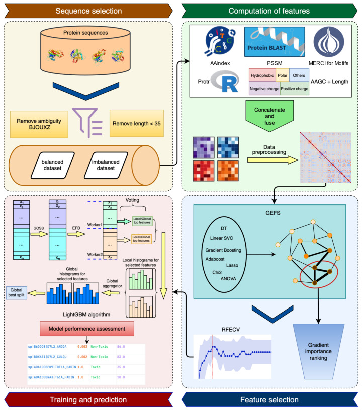 Figure 1
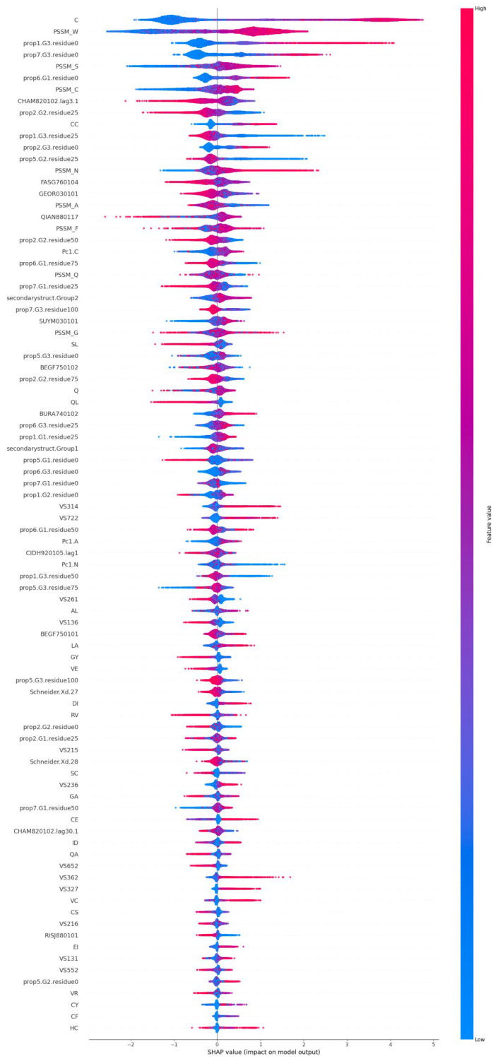 Figure 2
- —Suzhou Key Lab of Multi-modal Data Fusion and Intelligent Healthcare
Peer Reviews
No public reviews on file for this paper yet. If you reviewed it on a platform where reviews are public (OpenReview, ICLR, NeurIPS, ICML), you can paste yours below so the community can read it here.
Videos
No videos yet. Explain this paper in a talk, walkthrough, or lecture? Add one.
Taxonomy
TopicsComputational Drug Discovery Methods · Bacillus and Francisella bacterial research · Protein Structure and Dynamics
1. Introduction
Toxins are natural chemical compounds, peptides and proteins produced in all three kingdoms of life. They are poisonous substances to living organisms, sometimes including the toxin-producing organism itself. Venoms (zootoxins) contain up to hundreds of different compounds [1]. They are actively injected via bite or sting, or obtained, for example, by eating a venomous producer or through contact exposure. Venoms have multiple functions, often with many of them simultaneously, and are primarily contributed by different compounds and their combinations. The main function is to facilitate feeding. Another common purpose is defence. There are several other uses, usually limited to some organisms; see [1,2].
Venomous animals include snakes, spiders, scorpions, cone snails, centipedes, jellyfish, insects, sea anemones, lizards, fish, and platypuses. Many microbes and plants produce toxic compounds. Venoms have appeared in evolution at least 101 times [2]. The number of venomous animals is not known, but they appear in at least eight phyla [2].
Venoms pose a risk to humans. Venom effects are variable [3] and include cytotoxicity (causing cell and tissue damage, including necrosis), hemotoxicity (bleeding, blood clotting), and neurotoxicity (transmission of neural pulses), in addition to systemic effects, especially pain, swelling, in the most severe cases, respiratory failure, organ damage, and death. Effects can be mild and localised, severe or even life-threatening.
It has been estimated that annually, approximately 100,000 people die from snake venom out of 2.7 million who are bitten [4]. Some 300,000 obtain disabling consequences. Other venomous organisms cause further cases. Some venom toxin derivatives are used as drugs [5,6] and there are several potential application areas; for a review, see Ref. [7]. Antivenom is a molecule that binds to the venom components, obstructing them, which prevents the venom from reaching its target cells, tissue or organ. Antivenom does not reverse the effects of venom; instead, it prevents further damage by filtering out unused toxins. Recently, artificial intelligence has started to be used in the design of antivenoms [8],
The toxicity of venom compounds has been widely studied, but details are known only for a limited number of compounds. Experimental methods provide the most reliable data, but since they are laborious, time-consuming, and expensive, computational approaches have gained popularity. Based on the existing knowledge, prediction methods have been developed to detect and identify toxin molecules. The tools can be classified into several categories. There are dedicated predictors for the toxicity of small compounds, including eToxPred [9], MolToxPred [10], ProTox-II [11], toxCSM [12], ToxMPNN [13], and ToxinPredictor [14].
Toxin-specific predictors include BTXpred for bacterial toxins [15], Deep-STP for snake toxins [16], DeTox [17] for venomous toxins, NTXpred for neurotoxins [18], and SpiderP to spider toxins [19].
Generic toxin predictors can be divided into peptide and protein toxin predictors. Amp-toxicity [20], ATSE [21], ClanTox [22], tAMPer [23], ToxGIN [24], ToxIBTL [25], and ToxinPred 3.0 [26] are for peptide toxins. CSM-Toxin [27], NNTox [28], ToxClassifier [29], ToxDL [30], TOXIFY [31], ToxinPred2 [32], and VISH-Pred [33] are for protein toxins.
We present a novel machine learning (ML)-based predictor for protein toxins. We collected an extensive feature set and applied it to a large set of toxin and non-toxin proteins obtained from UniProtKB. The gradient boosting algorithm demonstrated the best performance, outperforming existing tools in comparison.
2. Results
Although several methods are available for predicting protein toxicity, there is still room for performance improvements. We collected a large dataset of toxic and non-toxic proteins from UniProtKB [34]. Toxic proteins have been annotated in the database as such. The non-toxic proteins contain all types of proteins except those that are toxic or allergenic.
We used an innovative approach to select representatives for the non-toxic proteins. The sizes of the two datasets were so different that choosing cases among the non-toxic proteins was necessary. We used clustering-based sampling, which exposed the predictor to a more diverse range of negative samples representing various clusters in the feature space. First, we employed the elbow method to determine the optimal number of clusters (see Supplementary Figure S1) and then selected representatives from each cluster. This way, the negative set also included rare or less frequent sequences, which might have been overlooked if random sampling had been used. When the number of clusters was 8, the decline rate of the SSE curve was markedly reduced, indicating a transition from a steep drop to a more gradual flattening. We selected 8412 sequences from the 8 clusters. The method divided the sequences for non-toxic proteins into clusters based on their feature distributions.
Figure 1 shows the flowchart for the method development. A large number of features in six different areas were collected and used to describe the proteins. Feature selection was employed to identify a concise list of the most important features for training. Four algorithms were tested, and the best one was chosen to train the ProToxin method, which was then compared to the state-of-the-art methods.
2.1. The Choice of Algorithm
With the complete set of features, we trained four algorithms. We tested RF, SVM, and two versions of gradient boosting. All these algorithms have gained popularity in bioinformatics.
The results for the 20-fold CV are shown in Table 1. The gradient boosting predictors were clearly superior to the RF and SVM. A sensitivity of 0.871, PPV of 0.923, accuracy of 0.899, MCC of 0.800, OPM of 0.7281, and F1 of 0.896 were the best for XGBoost, but LightGBM was very close. The scores indicate an excellent performance.
We had a total of 16,824 proteins in the training set, which were described in 2614 dimensions. The number of toxin and non-toxin proteins was equal. All algorithms were run with default parameters. The XGBoost algorithm had the highest score among all metrics (Table 1). The SVM had the poorest performance and was clearly the slowest to run. RF was the fastest to train, but its performance was lower than that of the boosting methods.
2.2. Features and Feature Selection
We collected a large set of features (see Supplementary Table S1); therefore, feature selection was necessary to identify only those features that contribute to the prediction. Feature selection was performed in successive steps. We started by removing 16 features that had zero standard deviations. These features did not provide any information about the proteins. Then, all the features were compared to identify those that were correlated. For all feature pairs, we calculated the Pearson correlation. If the coefficient was ≥ 0.8, only one of the correlated features was retained. In this step, we deleted 1081 features, leaving us with 1517 features. LightGBM was used for feature selection since it is fast to learn. We employed feature selection with an ensemble method and obtained 100 features. The final set of features was obtained by applying RFECV to the top 100 features, yielding optimal performance with 88 features, as shown in Table 2.
Table 2 presents the results for various feature types and their combinations. There were only 20 PSSM features, one per amino acid. It showed a surprisingly good performance. Minimotifs were another feature with small numbers, 50. They were inferior in separating toxins from non-toxins. PPV and specificity were perfect for a method trained on minimotifs; however, all the other scores were the worst among the tested feature sets. Even amino acid groups and normalised sequence length with just seven features were substantially better. The best performance was achieved with 88 features from different categories. Specificity was somewhat better than sensitivity, 0.942 vs. 0.883. Still, the method can be considered quite balanced in performance. An accuracy and AUC of 0.912, and an MCC of 0.827 indicate a reliable predictor.
The selected features are listed in Table 3. The largest number of features was for protr-based composition/transition/distribution (CTD) descriptors, with 29 features, followed by dipeptide composition descriptors (21), conjoint triad descriptors (12), and AAindex and PSSM parameters (both 8). CTD features convert protein sequences into fixed-length numerical feature vectors based on their amino acid properties. Dipeptide composition features are for enrichment/depletion of dipeptides in sequences. To calculate the conjoint triad descriptors, first, amino acids are classified into seven groups based on their properties. Triads of these seven groups are used for 343-dimensional vectors that contain the frequencies of each continuous triad within a sequence.
The importance of the features was visualised with the Shapley plot (Figure 2), which shows the importance of each feature in predicting toxic (positive values) and non-toxic (negative values) proteins. The features were arranged in order of decreasing importance. The blue colour indicates low values, and the red colour represents high values. The scale to the right indicates the increasing feature value.
The most important features are composition for C, sequence conservation PSSM scores for W, S and C. Among the selected features are two amino acid scores (for C and Q), 20 dipeptide scores, 8 PSSM values, and 8 AAindex values. Numerically, the largest group was the distribution descriptor. These features provide the position percentage in the entire sequence for the first residue, as well as 25%, 50%, 75%, and 100% residues for a certain encoded class. Among the top 10 most important features, four belong to this category. The physicochemical AAindex parameters describe various properties of amino acids. The significant parameters include those describing secondary structural elements (QIAN880117, BEGF750102, BURA740102, BEGF750101), linker propensities (GEOR030101, SUYM030101), pK values (FASG760104), and sequence conservation (RISJ880101).
Most of the features make the biggest contribution to toxin prediction, but there are, e.g., several frequency features for which small scores contribute to toxicity; see Figure 2. The Shapley plot summarises the importance of the selected features and provides information on how the scores are distributed among toxin and non-toxin proteins.
2.3. Method Development
To distinguish between LightGBM and XGBoost, which had very similar performances, we trained predictors using the selected 88 features and compared them on the blind test set, as shown in Table 4. The results are again very similar; however, XGBoost was chosen since it had a somewhat better overall performance. We call the final predictor ProToxin.
After selecting the best algorithm, we performed Bayesian hyperparameter optimisation of the XGBoost tool with cross-validation and trained the final predictor. The blind test set, an independent data set, was used for the final performance assessment. The accuracy was 0.906, the MCC was 0.797, and the OPM was 0.728. The scores for the blind test set are only marginally lower than those in feature selection; see Table 2.
2.4. Comparison to Other Methods
The blind test set was used to compare the performance of ProToxin to that of other available tools (Table 4). The comparison was made to five tools. For ToxinPred2, we tested two versions. ToxIBTL is a peptide toxin predictor; however, it was included in the comparison because it applies to proteins of up to 50 amino acids in length, and it was of interest to test whether it could extrapolate to proteins in general. Toxify and ToxIBTL are deep learning-based methods that utilise amino acid physicochemical propensities and evolutionary details. CSM-Toxin and VISH-Pred utilise language models: CSM-Toxin uses a bidirectional encoder representation from transformers (BERT), and VISH-Pred uses an ESM2 transformer model. ToxinPred2 is an RF model trained on many features, similar to ProToxin.
Apart from PPV and specificity, ProToxin performs markedly better than the competing tools. CSM-Toxin has the best scores for PPV and specificity, 0.976 and 0.989, respectively. However, this was achieved at the expense of severely biased performance. The scores for NPV and sensitivity are 0.861 and 0.728, respectively. A good predictor exhibits a well-balanced performance with minimal differences between the measures. The accuracy of CSM-Toxin was the second best after ProToxin. The MCC value was 0.774, and the OPM was 0.701. The ToxinPred2 hybrid version was the third-best method, followed by ToxinPred2.
MultiToxPred has the poorest performance with an accuracy of 0.598, MCC of 0.196, OPM of 0.201, and F1 of 0532. Interestingly, the peptide predictor ToxIBTL performed better despite being trained on shorter sequences; see Table 4.
2.5. ProToxin Server
ProToxin is available as an online platform. Users can manually enter or alternatively upload protein sequence(s) in FASTA format, upon which ProToxin retrieves and processes the essential sequence data. ProToxin is freely available at https://structure.bmc.lu.se/ProToxin/ (accessed on 26 September 2025) and https://www.yanglab-mi.org.cn/ProToxin/ (accessed on 26 September 2025). The datasets used for training are available at the websites.
3. Conclusions
We developed a novel gradient boosting-based predictor for protein toxicity. The method was trained on carefully selected training data. We employed a clustering approach to efficiently cover the space of non-toxic sequences. Initially, we tested a long list of various types of features, which were reduced to 88 after a comprehensive feature selection procedure. Out of the four tested algorithms, XGBoost was chosen to train the final predictor. Comparison to available predictors indicated that ProToxin showed significant improvement compared to state-of-the-art predictors. ProToxin is a fast and efficient method and is freely available. It can be used for small and large numbers of sequences. As experimental studies are expensive and time-consuming, ProToxin can provide a rapid assessment of toxicity. The tool could also be used for primary safety screening of sequencing-project-derived proteins and even designed proteins.
4. Materials and Methods
4.1. Data Collection and Cleaning
Data for venoms and toxins were collected from UniProtKB [34] (https://www.uniprot.org/) and downloaded on 9 September 2024. Sequences in FASTA format were retrieved using the keyword “KW-0800” for toxic proteins. Entries labelled as “reviewed” were selected. A reverse keyword-based search was employed to find a negative protein dataset. Sequences annotated with the keywords KW-0800 or KW-0020 (indicating allergenic proteins) were excluded. The sequences had a reviewed status. In both groups, sequences shorter than 35 amino acids were removed, and protein sequences containing ambiguous or nonstandard amino acids B, J, O, U, X, or Z were filtered out.
The training dataset contained 8412 toxins and 246,092 negative samples as non-toxins. An independent blind test set included 279 toxins and 474 non-toxins. Datasets are available at the predictor website.
There were many more non-toxic proteins than toxic ones. Therefore, we generated a balanced dataset. We applied the K-means clustering algorithm to the negative set. We clustered the sequences into 2 to 20 clusters (k values) and used the elbow method to evaluate the curve of the sum of squared errors (SSEs) as a function of k:
where denotes the sample that belonged to the j cluster; cj denotes the centre of the j cluster.
The balanced dataset was used to train the model. The positive and negative sequences were randomly divided into 20 subsets for cross-validation. In each split, 95% of the data was allocated for training, while the remaining 5% was reserved for validation. The performance evaluation of the cross-validation was calculated as the average result across 20 folds.
4.2. Features
We collected a large number of features belonging to six major groups, including protr-based features [35], PSSM scores, amino acid group counts [36], sequence length, AAindex features [37], and sequence motifs [38].
Protr program 1.7-4 [35], an R package v. 4.4.2, was used to generate most sequence-based features. With protr, we calculated features in 8 descriptor groups and obtained 1920 features altogether.
We used Psi-BLAST 12.14.0+ [39] to determine position-specific scoring matrices (PSSMs) based on evolutionary information. We searched for each protein against UniProtKB. The E-value threshold was set to 0.001, and the number of iterations was set to three. We used the global average pooling (GAP) method [7] to compress the irregularly shaped PSSMs into (1, 20).
Due to the varying lengths of each protein sequence, the shapes of the PSSMs differed. The matrix shape was (L, 20), where L is the number of amino acids in a protein. Using GAP, we mapped and concatenated the different matrices into the same shape (1, 20).
where L denotes the sequence length and P_i,j_ represents the score of the j-th amino acid at position i in the sequence.
Amino acid group counts and sequence length. Amino acids were divided into six groups according to their physicochemical properties as follows: hydrophobic (V, I, L, F, M, W, Y, and C), negatively charged (D and E), positively charged (R, K and H), conformational (G and P), polar (N, Q and S) and others (A and T) [36]. We counted the numbers in the six groups and the sequence length. In this category, there were a total of seven features.
Sequence minimotifs were identified with Motif-EmeRging and with Classes-Identification (MERCI) [38]. We identified 50 motifs that appeared in the toxin proteins but not in the non-toxic ones. A one-hot method was used, creating a vector of 50 elements for each sample.
In total, we collected 2614 features for each protein.
4.3. Feature Selection
We used a two-step feature selection. First, we removed columns with a standard deviation of 0 for features where all samples had the same value. Then, we performed a pairwise Pearson correlation analysis on the remaining features using the following formula:
where x_i_ and y_i_ were the ith variables of features X and Y, respectively. and were the mean values for X and Y, respectively. If the correlation coefficient between the two features was ≥0.8, the two features exhibited a strong correlation, and one was removed.
Graphical ensembling theory [40] was used to identify the most important features among the remaining features with a co-selection graph, where vertices represented features and edges were weighted by the number of times the features were selected together, allowing for the training of several ML algorithms. We used recursive feature elimination with cross-validation (RFECV) [41] to obtain the final set from the top 100 features.
4.4. Model Architecture
We tested several ML algorithms, including random forests (RF), support vector machines (SVM), and two versions of gradient boosting methods: XGBoost and LightGBM. A 20-fold CV was used to identify the best-performing algorithm.
The ML algorithms utilised Python Scikit-learn 1.2.1 scripts and employed default parameters. We adopted a strict nested cross-validation approach and implemented an end-to-end, reproducible workflow using a Scikit-learn pipeline. This ensured that any step utilising label information was learned only with the training portion of each outer fold, and that transformations were applied only to the test portion of that fold, thereby preventing information leakage.
RF is an ensemble learning method based on decision trees [42]. It constructs multiple decision trees and aggregates their predictions through voting (for classification) or averaging (for regression). It is resistant to overfitting and robust to noisy data. It uses random feature selection and bootstrapped samples to construct multiple decision trees, improving generalisation. It can be computationally expensive with a large number of trees.
SVM is a supervised learning algorithm for classification and regression [43]. It finds the optimal hyperplane that maximises the margin between different classes. Kernel methods enable the effective handling of nonlinear classification problems. It also works well with small datasets and high-dimensional data.
XGBoost is an ensemble learning method based on gradient boosting that uses weighted decision trees for modelling [44]. It improves efficiency through optimisations like second-order derivative calculations of the loss function and regularisation techniques, balancing accuracy and computational performance.
LightGBM (Light Gradient Boosting Machine), developed by Microsoft in 2017, is optimized for large-scale data and high-dimensional features [45]. It utilizes GOSS (Gradient-based One-Side Sampling) to prioritize high-gradient samples and EFB (Exclusive Feature Bundling) to merge rarely co-occurring features, thereby boosting speed and reducing memory usage. It is much faster and lighter than XGBoost, and it supports parallel learning, GPU acceleration, and automatic handling of missing values.
4.5. Performance Assessment
We used 10 measures to describe the performance of models, including accuracy; area under the curve, AUC; F1 measure; negative predictive value, NPV; positive predictive value, PPV; Matthews correlation coefficient, MCC; overall performance measure, OPM; sensitivity; and specificity.
TP and TN are correctly predicted toxic and non-toxic cases, respectively, and FN and FP are the numbers of incorrect predictions for toxic and non-toxic cases, respectively.
The reference list from the paper itself. Each links out to its DOI / PubMed record.
- 1Utkin Y. Animal Venoms and Their Components: Molecular Mechanisms of Action Toxins 20211341510.3390/toxins 1306041534207957 PMC 8230695 · doi ↗ · pubmed ↗
- 2Schendel V. Rash L.D. Jenner R.A. Undheim E.A.B. The Diversity of Venom: The Importance of Behavior and Venom System Morphology in Understanding Its Ecology and Evolution Toxins 20191166610.3390/toxins 1111066631739590 PMC 6891279 · doi ↗ · pubmed ↗
- 3White J. Venomous animals: Clinical toxinology EXS 201010023329110.1007/978-3-7643-8338-1_720358686 · doi ↗ · pubmed ↗
- 4Gross M. The venom menace Curr. Biol.202333 R 1209 R 121210.1016/j.cub.2023.11.029 · doi ↗
- 5Waheed H. Moin S.F. Choudhary M.I. Snake Venom: From Deadly Toxins to Life-saving Therapeutics Curr. Med. Chem.2017241874189110.2174/092986732466617060509154628578650 · doi ↗ · pubmed ↗
- 6Smallwood T.B. Clark R.J. Advances in venom peptide drug discovery: Where are we at and where are we heading?Expert Opin. Drug Discov.2021161163117310.1080/17460441.2021.192238633914674 · doi ↗ · pubmed ↗
- 7Kim E. Hwang D.H. Mohan Prakash R.L. Asirvatham R.D. Lee H. Heo Y. Munawir A. Seyedian R. Kang C. Animal Venom in Modern Medicine: A Review of Therapeutic Applications Toxins 20251737110.3390/toxins 1708037140864047 PMC 12390438 · doi ↗ · pubmed ↗
- 8Callaway E. AI-designed proteins tackle century-old problem—Making snake antivenoms Nature 202563777610.1038/d 41586-025-00133-z 39814930 · doi ↗ · pubmed ↗