Addressing Parameter Variability in Corneal Biomechanical Models: A Stepwise Approach for Parameters’ Optimization
José González-Cabrero, Carmelo Gómez, Manuel Paredes, Francisco Cavas

TL;DR
This paper introduces a stepwise method to optimize corneal material model parameters, aiming to reduce variability and improve reliability in biomechanical modeling.
Contribution
A novel stepwise approach is proposed to separately estimate isotropic and anisotropic components in corneal biomechanical models.
Findings
The stepwise approach reduces variability in parameter sets by isolating isotropic and anisotropic components.
The methodology improves the reliability of corneal material model parameters for clinical and biomimetic applications.
Abstract
Biomechanical modeling of the cornea is crucial for understanding the progression of some ocular diseases and optimizing surgical treatments. However, hyperelastic non-linear material models, such as those used for corneal tissue, often yield highly variable parameter sets in the scientific literature, influenced by factors like the chosen optimization intervals and differences between tensile and inflation test curve optimization, both of which are addressed in this study. This variability complicates the understanding of corneal mechanical properties. In this research, the aim is to optimize and calibrate the key parameters of the corneal material model, particularly focusing on c1, c2, k1 and k2, using the Holzapfel–Gasser–Ogden (HGO) hyperelastic model, and a novel methodology is proposed that separately estimates the isotropic and anisotropic components in a stepwise manner,…
Genes, proteins, chemicals, diseases, species, mutations and cell lines named across the full text — each resolved to its canonical identifier and authoritative record.
Click any figure to enlarge with its caption.
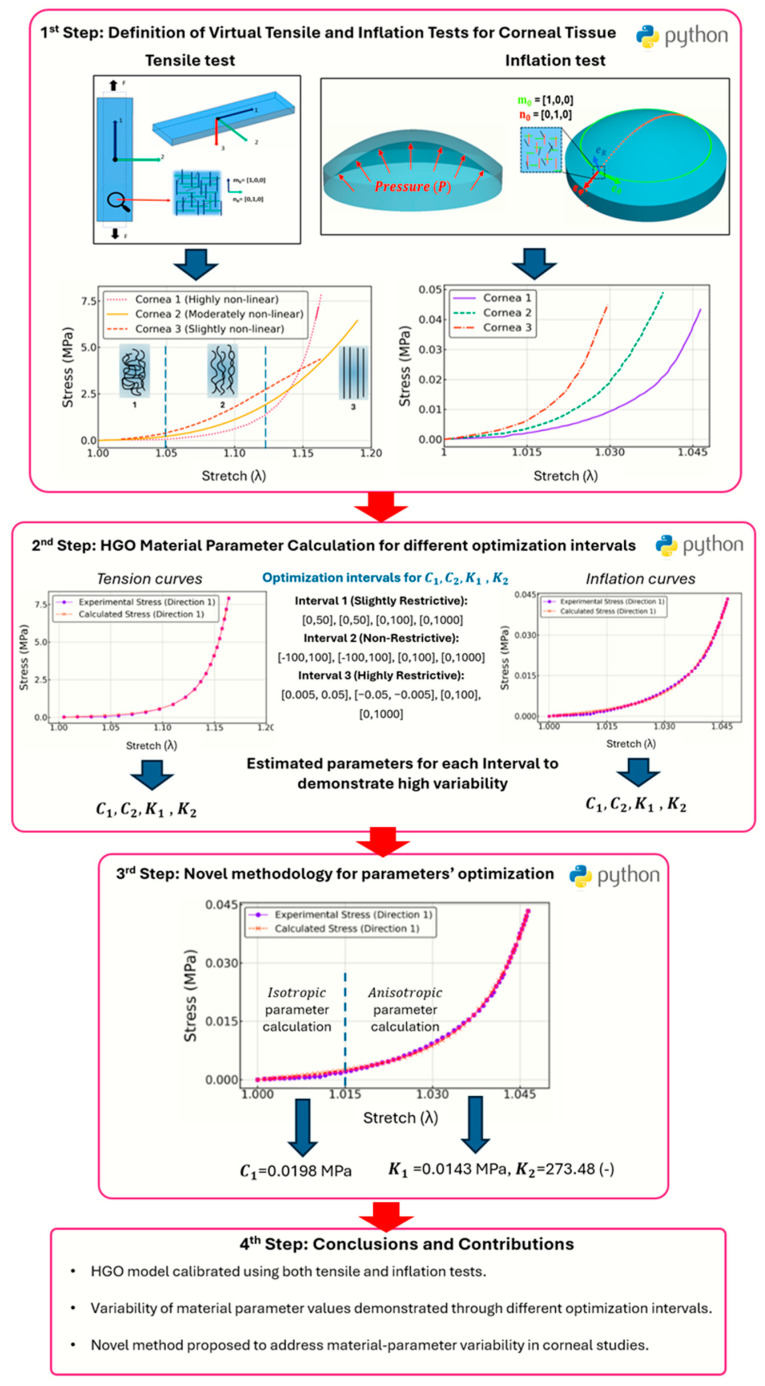 Figure 1
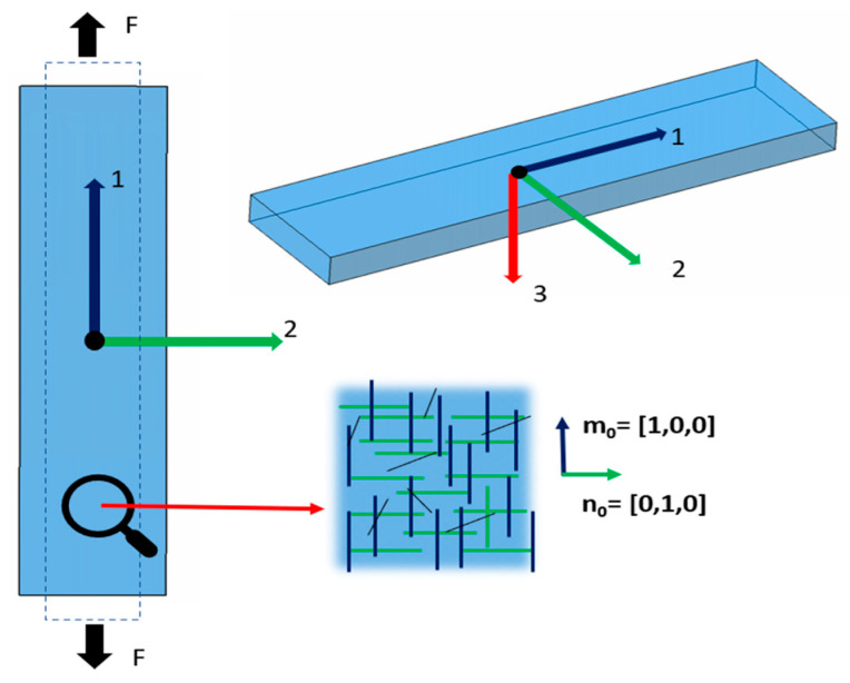 Figure 2
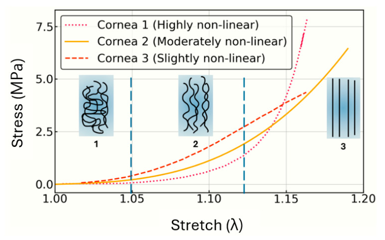 Figure 3
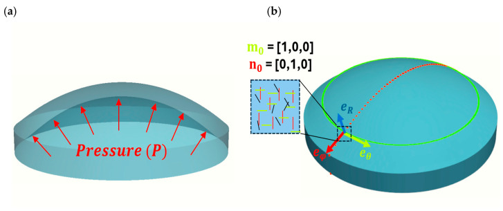 Figure 4
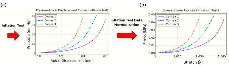 Figure 5
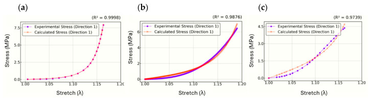 Figure 6
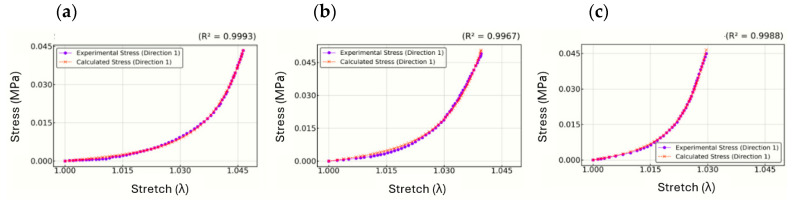 Figure 7
- —research project 22665/PI/24
- —Association for the Integration of the Disabled in the Comarca del Mar Menor
Peer Reviews
No public reviews on file for this paper yet. If you reviewed it on a platform where reviews are public (OpenReview, ICLR, NeurIPS, ICML), you can paste yours below so the community can read it here.
Videos
No videos yet. Explain this paper in a talk, walkthrough, or lecture? Add one.
Taxonomy
TopicsCorneal surgery and disorders · Ophthalmology and Visual Impairment Studies · Corneal Surgery and Treatments
1. Introduction
The human eye receives over 90% of external sensory information, highlighting the critical importance of ocular health for quality of life [1]. The cornea, contributing approximately two-thirds of the eye’s refractive power [2], plays a vital role in this process. This avascular structure, with an average thickness of 550 μm centrally and 750 μm peripherally, is primarily composed of stroma, which accounts for 90% of its thickness and consists of collagen fibers embedded in a proteoglycan matrix and arranged in a region-specific orientation [3].
The cornea’s mechanical behavior is commonly modeled using anisotropic hyperelastic models [4,5], essential to optimize surgical outcomes and understanding diseases like ectasia, characterized by structural weakening of collagen fibers [6]. Hyperelastic models, such as the Gasser–Holzapfel–Ogden (GHO) and Holzapfel–Gasser–Ogden (HGO) models, have become standard in corneal studies due to their capacity to describe anisotropic properties and fiber dispersion [7,8,9,10]. These models assume near-incompressibility and provide parameters representing isotropic stiffness, fiber stiffness, and non-linear deformation. However, parameter variability across studies, influenced by differences in experimental techniques, tissue properties, and mathematical simplifications, complicates direct comparisons and the reliability of conclusions between studies [11,12,13,14].
Tensile and inflation tests are the primary experimental methods to estimate corneal parameters. However, the two approaches yield inconsistent results due to differences in testing conditions and the mathematical models applied. For example, studies using tensile tests, such as those by [11,12,13], have reported wide variability in parameter values, while inflation tests, as demonstrated by [14,15], highlight the sensitivity of material parameters to experimental conditions.
Experimental comparisons have shown that strip extensometry and inflation produce markedly different responses [16] and that multiple loading scenarios are critical for accurate parameter identification [17]. Moreover, recent advances such as Brillouin microscopy have enabled non-invasive biomechanical characterization [18], while age- and IOP-related collagen recruitment studies further emphasize the variability in corneal mechanical response [19]. Recent ex vivo and animal studies also demonstrate discrepancies between uniaxial and biaxial testing outcomes [20], highlighting the difficulty of establishing universally valid parameter sets.
Variations in geometric measurements, non-uniformity of corneal properties, and model-specific assumptions contribute to these discrepancies. Furthermore, high correlations between experimental data and model predictions (high correlation coefficients ) do not always ensure unique or physically valid parameter sets. This issue arises when parameter compensations occur, leading to multiple sets that fit experimental data similarly. Consequently, it becomes necessary to establish robust methods for parameter estimation that minimize variability and improve reliability.
This study aims to address these challenges by (1) developing a method to characterize corneal material parameters of the HGO model through a novel stepwise optimization approach that separates the estimation of the isotropic ground-matrix components from the anisotropic fiber parameters to reduce variability and ensure physical consistency in the estimated parameters; (2) proposing parameter bounds and optimization algorithms to demonstrate the high variability inherent in the characterization problem, driven by the large number of parameter combinations that yield similarly high correlation with the experimental curve.
Beyond its clinical relevance, this research also fits within a biomimetic perspective. The cornea, combining transparency, anisotropy, and mechanical resilience, serves as an inspiring model for bioengineered materials. Advances in contact lenses, tissue substitutes, and artificial corneal constructs seek to replicate these properties, highlighting how biomechanical modeling can guide the design of biomimetic solutions that emulate their structural and functional efficiency. In this context, an accurate characterization of the cornea’s hyperelastic properties is essential to ensure that such designs achieve physiological-like behavior.
2. Materials and Methodology
In this research, a detailed methodology is implemented to optimize the material parameters of corneal tissue ( , , and ) using tensile and inflation tests within the Holzapfel–Gasser–Ogden (HGO) model framework [7]. This model is adopted because it combines physiological realism with simplicity: it separates the isotropic ground matrix ( , ) from collagen–fiber reinforcement and reproduces the cornea’s characteristic exponential stiffening ( , ). Other models, such as the five-parameter Mooney–Rivlin formulation [21], can also capture pronounced nonlinearity; however, they make it more difficult to distinguish which parameters govern the initial, matrix-dominated segment of the curve and which govern the later, fiber-driven non-linear response.
Both tensile and inflation tests are mathematically defined to simulate the cornea’s mechanical behavior under physiological conditions. The methodology is summarized in the scheme shown in Figure 1.
Python version 3.11.9 (Python Software Foundation) is used for data analysis, parameter optimization, and curve fitting. Core libraries were NumPy for array algebra, SciPy (differential_evolution, best/1/bin) for parameter optimization, and Matplotlib for plotting.
In the optimization process, a differential evolution algorithm is employed to iteratively adjust the material parameters ( , , and ) to minimize the difference between the predicted stress values ( , , ) and the experimental data.
This approach, known as least-squares minimization, aims to reduce the total error in the predicted stress values. Penalties are also introduced to avoid physically meaningless solutions, such as negative stress values ( ), ensuring that the parameters remain physically valid throughout the optimization process. The coefficient of determination, is used to evaluate the quality of the fit between the model’s predictions and the experimental data; it measures how much of the variance in the experimental data is captured by the model, with a value close to 1 indicating a strong fit.
The optimization analysis is conducted by implementing three different parameter bounds to demonstrate that various parameter sets can achieve high experimental fits with values close to 1, while still maintaining physical validity in order to explain the variability of parameter sets commonly reported in the literature. The goal is to analyze which parameter interval is preferable, ranging from highly restrictive, moderately restrictive, to non-restrictive bounds. Only different intervals are set for and , while maintaining for , and . The optimization process is iterated within these intervals until the set that minimizes the error is found.
Experimental data for the tensile and inflation tests’ curves are obtained from published investigations. To mitigate inconsistencies and enhance parameter stability, a stepwise optimization approach is proposed in Section 3.3. First, is optimized for small deformations dominated by isotropic behavior. Once is established, and are optimized to capture the anisotropic non-linear behavior at larger deformations, while is neglected. This sequential approach simplifies the optimization process and reduces parameter variability, addressing a major limitation in prior studies. By first fitting on the small-strain, matrix-dominated segment and then fitting and on the non-linear, fiber-dominated segment, the estimation is split into lower-dimensional subproblems, which removes many compensating parameter combinations and thereby reduces parameter variability even when remains high.
2.1. Biomechanical Modeling of Corneal Material
In hyperelastic material modeling, the local deformation is described by the deformation gradient , which maps a material point from its reference position to its current deformed position . Its determinant is the local volume ratio; for incompressible response, J = 1 (volume preservation). The Cauchy stress tensor is written as
where is the Cauchy stress tensor, is a Lagrange multiplier that enforces incompressibility and represents the hydrostatic/volumetric part of the stress, and I is the identity tensor (unit tensor) that produces an equal normal contribution in every direction. The symbol denotes the strain–energy density function. The tensor C = is the right Cauchy–Green deformation tensor, which measures strain in the reference configuration. The derivative is the tensor of partial derivatives of the energy with respect to C. In practice, ψ is often split into a volumetric term and a deviatoric (shape-changing) term. In this work, incompressibility is enforced by the Lagrange multiplier , so the volumetric contribution is represented by the hydrostatic term in Equation (1); therefore, ψ in Equation (1) denotes only the deviatoric strain-energy density. The deviatoric component of in the HGO model is as follows:
where + defines shear modulus, describes fiber stiffness, and accounts for nonlinearity in large strains. The invariants are , , and , where and are initial fiber directions.
Assuming incompressibility and following the theory of continuum mechanics, the Cauchy stress tensor can be expressed in terms of the invariants and the left Cauchy–Green deformation tensor through the following expression:
where and are the orientation vectors in the preferred directions in the deformed configuration, and is the identity matrix.
Tensile Test
During the tensile test, the tissue is clamped at both ends, and a tensile force is applied along the length in the 1-direction, resulting in elongation characterized by the stretch ratio > 1. To maintain volume due to incompressibility, the tissue contracts in directions 2 and 3 perpendicularly. The deformation gradient tensor is given by
where ensures incompressibility. For a tensile load in the 1-direction, with the tissue confined to the 1–2 plane, and . The Cauchy stress tensor is expressed as follows:
For uniaxial tensile tests, stress is applied only in the 1-direction, so ; . Figure 2 illustrates the virtual tensile setup where the specimen is clamped at both ends and loaded along direction 1.
Tensile strips are typically cut along the inferior–superior or nasal–temporal anatomical axes; these are widely considered the principal corneal fiber directions in the central stroma of the cornea; to generalize across published datasets, this orientation is assumed for all cases. Accordingly, two preferred in-plane fiber families are defined and taken orthogonal in the reference configuration: aligned with the loading direction and aligned transversely. The local axis {1, 2, 3} is also indicated in the figure.
The schematic Figure 3 represents the stress–stretch curves used in this research for three different corneal specimens under tensile testing obtained from [13,14], highlighting varying degrees of non-linearity in their mechanical responses. Additionally, it illustrates the collagen fiber alignment during the stretching process in three stages.
2.2. Inflation Test
The inflation test is critical to understand the cornea’s biomechanics, as it closely replicates in vivo conditions by applying pressure similar to intraocular pressure (IOP). Unlike uniaxial tensile tests, it provides insights into the realistic mechanical response of corneal tissue under physiological conditions. Note that an axisymmetric thin-membrane assumption is adopted to match the experimental inflation setup and as a test simplification, implying equibiaxial loading ( ). The cornea, however, is not a perfect spherical cap and exhibits regional variation and fiber dispersion; these aspects are acknowledged in Section Limitations of the Study. The deformation gradient tensor for the inflation test is
where λ_1_, λ_2_, and λ_3_ are the stretches in the meridional , circumferential and radial directions, respectively. Due to incompressibility, = and = , with .
Assuming a thin-membrane model, the cornea is treated as sufficiently thin to neglect through-thickness stresses and bending effects in the radial direction , resulting in a biaxial stress state in the meridional and circumferential directions. The stress tensor is as follows:
where represents the stress in both directions. This setup allows studying corneal behavior under applied pressure, as shown in Figure 4.
The equations to convert pressure–apical displacement data into stress–stretch relationships are detailed in Appendix A according to [22]. These include the conversion of pressure units, calculation of the radius of curvature and stretch, and the application of Laplace’s law to determine corneal stress. The equations account for geometric changes in the cornea during deformation, assuming it behaves as a spherical shell. Figure 5 shows the transformation of the curves [10] before and after applying the normalization process.
2.3. Parameter Optimization for Tensile and Inflation Tests
The four parameters ( , , and ) are fitted simultaneously using the differential evolution algorithm (strategy best/1/bin), implemented in Python via SciPy (from scipy.optimize import differential_evolution). This algorithm efficiently handles complex, non-linear problems typical of hyperelastic material modeling. The optimizer minimizes a least-squares error between model predicted and experimental stresses, augmented with large penalties to enforce test physics: penalties avoid negative stress, and non-monotonic axial stress as stretch increases.
The algorithm runs up to 10,000 iterations with a tolerance of 1 × 10^−6^ on the objective. Parameter bounds are implemented as box constraints; their restrictiveness is varied to demonstrate that different intervals can yield different parameter sets, with further discussion provided in Section 3. Goodness of fit is reported with the coefficient of determination (where is the residual sum of squares (predicted vs. experimental), and is the total variance in experimental data).
Section 3.3 introduces a novel stepwise approach seeking to stabilize parameter identification by separating the estimation of the isotropic part ( ) from the anisotropic part ( and ).
3. Results
3.1. Parameter Optimization: Tensile Test
In the optimization process, three bound intervals are tested (Interval 1 (slightly restrictive), Interval 2 (non-restrictive), and Interval 3 (highly restrictive)) to demonstrate how bound choices affect the resulting parameter sets.
The rationale for the bounds selection is explanatory (to show how bounds affect identifiability), keeping the fiber terms effectively unrestrictive ( in [0, 100] MPa and in [0, 1000]) while varying only the isotropic bounds. Interval 1 (“slightly restrictive”) uses positive-only ranges for and (e.g., [0, 50] MPa); whether the upper limit is 50 or 100 MPa is immaterial, provided the range is sufficiently large to calculate without restriction. Interval 2 (“non-restrictive”) allows and in [−100, 100] MPa, admitting negative values, sometimes reported to compensate ; any solutions with + ≤ 0 are deemed physically inadmissible even if the statistical fit is high. Interval 3 (“highly restrictive”) adopts narrow literature-based ranges around typical and values to illustrate how tight priors can over-constrain the fit and promote parameter compensation in and .
Interval 1 (Slightly Restrictive) provides the most reliable results, with parameter bounds of [0, 50] for and , and [0, 100] and [0, 1000] for and , respectively. This interval ensures physical validity, avoiding negative shear stress values ( + ). The algorithm consistently assigns near zero, simplifying the isotropic component to a single parameter ( ), which effectively captures the material’s initial stiffness. This interval results in high values while maintaining interpretability, with parameter values reflecting the stiffness and fiber behavior across different non-linearities of the corneal tissue.
Interval 2 (Non-Restrictive), with bounds of [−100, 100] for and , leads to unrealistic results, such as negative shear stress, rendering the parameters physically invalid despite high values. This demonstrates that overly broad bounds can cause overfitting, producing results that are statistically accurate but lack meaningful representation of material properties.
Interval 3 (Highly Restrictive) tightly constrains and to [0.005, 0.05] and [−0.05, −0.005], respectively, while maintaining the same bounds for and as in Interval 1. Although this interval produces physically valid results, it forces some parameters to their boundary values, leading to compensatory adjustments in and . While useful in specific scenarios where parameter ranges are well-defined, such tight constraints may limit the optimization process and risk over-constraining the system.
Results of the estimated HGO material parameters for the optimization intervals are shown in Table 1.
Figure 6 presents the stress–stretch curves for Interval 1 (Slightly Restrictive). Plot (a) corresponds to the highly non-linear curve, (b) represents the moderately non-linear curve, and (c) shows the slightly non-linear curve. It illustrates the correlation between the experimental stress and the predicted stress. The high values (ranging from 0.97 to 0.99) demonstrate an excellent fit between the experimental and calculated curve, confirming the accuracy of the optimization process.
The three datasets fitted in this section correspond to the literature tensile curves shown previously in Figure 3 obtained from [13,14]. Stresses in directions 2 ( ) and 3 ( ) are expected to remain zero, as required by the boundary conditions of a uniaxial tensile test, confirming that the parameter set obtained from Interval 1 produces physically meaningful and reliable results across all directions.
3.2. Parameter Optimization: Inflation Test
Results from the inflation test are visually represented in Figure 5b, where three corneas (Cornea 1, Cornea 2, and Cornea 3) are displayed. These curves reflect a typical stress–stretch behavior, showing increasing stiffness as stretch progresses. It can be observed that the sudden non-linear behavior, or “knee,” occurs at different points along the curves, with some corneas showing an earlier rapid increase in stiffness, while others present a more gradual transition.
Cornea 1 exhibits a gradual increase in stress at lower strains, followed by a sharper rise later on. This indicates that Cornea 1 shows delayed fiber stiffening, as it is dominated by a lower initial stiffness, influenced mainly by a lower . Cornea 2, on the other hand, displays a more intermediate response, with a smoother balance between early-stage stiffness and later non-linear behavior. Cornea 3 presents the sharpest increase in stress almost from the beginning of the test, which suggests that Cornea 3 has a higher initial stiffness (likely due to a higher ) and reaches the non-linear fiber-dominated region earlier than the others.
As in Section 3.1, the parameter optimization for the inflation test is carried out for three different intervals, from which the material parameters are optimized using the differential evolution algorithm. A detailed analysis of the set of parameters obtained for each interval and the strong correlation with the experiments are shown in Table 2, with values close to 1.
Interval 1 (Slightly Restrictive) emerges as the most suitable for parameter estimation due to its ability to provide physically meaningful values without encountering negative or unrealistic results. However, as shown in Table 2, all curves in this interval exhibit zero values for both and , effectively neglecting the isotropic contribution to the cornea’s material behavior. This simplification suggests that the model primarily captures anisotropic stiffening due to fiber alignment, which may not fully represent the cornea’s initial stiffness, as the isotropic matrix plays a critical role in early deformation responses. This limitation highlights the need for further refinement in optimizing , as addressed in Section 3.3.
In contrast, Interval 2 (Non-Restrictive) allows for a broader exploration of parameter values but yields physically invalid results. For example, Cornea 2 shows = 2.905 MPa and = −3.792 MPa, resulting in a negative shear modulus ( + ), which is inconsistent with the physical interpretation of the corneal material. Despite achieving high values, these results lack physical coherence and cannot reliably describe the cornea’s mechanical properties.
Interval 3 (Highly Restrictive), while yielding physically valid results, imposes excessively tight constraints that limit the optimization process. Parameters like are consistently forced to boundary values, such as = 0.005 MPa, restricting the model’s ability to explore the cornea’s true mechanical behavior. Although this interval may be useful in specific scenarios, its restrictive nature makes it less suitable for general applications.
Figure 7 illustrates the stress–stretch curves for the inflation test using parameters from Interval 1, with results presented for highly non-linear (a), moderately non-linear (b), and slightly non-linear (c) cases. The model accurately captures the anisotropic mechanical behavior of the cornea under inflation conditions. In plots (a, b, c), the predicted stress aligns closely with the experimental data, achieving high values ranging from 0.9967 to 0.9993. The circumferential and meridional stresses are equivalent, consistent with the equibiaxial tension assumption, while the radial stress remains near zero, as expected under thin membrane conditions. These findings confirm that the parameter set derived from Interval 1 provides a reliable and consistent representation of the cornea’s mechanical response.
3.3. Novel Methodology for Parameter Optimization in Corneal Inflation Tests
During the optimization process for the inflation test, it became clear that the values of were unrealistically low, being calculated as zero in some configurations. This is physically incorrect because is responsible for the isotropic stiffness of the corneal matrix, which plays a crucial role in the initial response to deformation. To address this issue, a strategy is implemented to refine the model and ensure more accurate values for .
The initial portion of the stress–stretch curves, where the response is approximately linear and dominated by the isotropic matrix, is isolated and optimized separately. This step allowed the model to focus on adjusting , ensuring that the early stiffness of the cornea is accurately captured. The exact cutoff for this linear segment can vary between curves, but a practical guideline is that collagen fibers begin to bear a significant share of the load at roughly 2% strain [20]. Therefore, the 0–2% strain range can be treated as approximately linear and dominated by the isotropic matrix.
After isolating the initial phase of the curves, strict limits close to zero are imposed on , and to refine the optimization of . It is important to remember that can be neglected to simplify the material model, reducing it to a system with only three parameters to optimize. The final values for are in Table 3, demonstrating a clear increasing trend from Cornea 1 to Cornea 3. This validates the method, as the graphs show a corresponding increase in initial stiffness, aligning with the expected mechanical behavior.
Once is fixed, the anisotropic parameters and are optimized to capture the non-linear behavior of the cornea. The resulting values reflecting the influence of fiber alignment and stiffening in the later stages of the stress–strain response are shown in Table 4:
Upon analyzing , there appears to be no clear trend across the curves (it increases from Curve 1 to Curve 2 but then decreases in Curve 3). This pattern suggests that does not solely govern the non-linear behavior of the cornea and likely interacts with both and , complicating its interpretation. In contrast, shows a clear increasing trend from Curve 1 to Curve 3, playing a more dominant role in the non-linear stiffening behavior observed at higher strains. This makes sense, as is closely linked to fiber stiffening. The overlap of ’s effects with both and complicates the optimization, reinforcing the importance of first optimizing to separate isotropic behavior from fiber-driven non-linearity. Once is fixed, and can be optimized more effectively.
In summary, increases steadily from Curve 1 to Curve 3, reflecting greater initial stiffness. follows a non-monotonic pattern, with no clear trend, while consistently rises, capturing the sharp increase in stiffness due to fiber alignment at larger strains, aligning with typical non-linear stiffening seen in the cornea during inflation tests.
4. Discussion
The significant variability observed in corneal biomechanical studies, particularly in tensile and inflation tests, arises from various causes. In this research, the authors highlight that these discrepancies mainly occur because different parameter sets can still make physical sense and achieve strong correlations with experimental data. This introduces challenges in defining a universally accepted set of material parameters for corneal tissues.
In tensile tests, a wide range of parameter values is reported across different studies (see Table 5). The parameters , , , and show considerable variability, reflecting the anisotropic stiffening behavior of the cornea under uniaxial loading conditions. For example, values range from 0.0025 MPa [13] to 15.11 MPa [10] (Hoeltzel et al., 1992), illustrating a great difference in the isotropic stiffness parameter. Similarly, spans from 0.0338 MPa [15] to 103.5 MPa [12] (M. Nambiar et al., 2022), showing a wide range in fiber alignment’s contribution to corneal stiffness. values vary from 5.74966 [13] to 1280.07 [15], highlighting a massive disparity in scale in the non-linear stiffening behavior of collagen fibers across the studies. These variabilities may also contribute to geometrical differences in the corneal specimens, testing different corneal regions (central vs. peripheral), variations in experimental conditions, and the methods used to model the anisotropic behavior of the tissue.
To aid comparison across sources, Table 5 (tensile) and Table 6 (inflation) use (−) to indicate values not reported. The differences across studies reflect model choices. Some studies use an HGO formulation with a two-parameter Mooney–Rivlin isotropic base ( and ), others report only a single isotropic parameter ( ), and some fit their curves with a pure two-parameter Mooney–Rivlin model without fiber terms and . For Table 6, note that [15] present a re-fit in which and are recalculated after fixing to the mean across specimens (0.004 MPa).
Inflation tests present distinct challenges. Variability in inflation studies is also very high (see Table 6). Apart from the previously mentioned possible sources of variability, an additional source arises from converting pressure–apical displacement curves into stress–stretch curves, which relies heavily on geometrical measurements such as the corneal base radius, thickness, and apex height. If these are measured inaccurately, they can drastically alter the resulting curves. Consequently, variation in material parameters in inflation tests stems from differences in these geometric inputs, in addition to model assumptions and experimental conditions. For instance, values in inflation tests range from 0.00291 MPa [15] to 0.32 MPa [10]. Similarly, values vary between 0.0217 MPa [15] and 0.055 MPa [10], and ranges from 291.28 [15] to 750 [10].
Tensile and inflation test parameters are not directly comparable. The mechanical behavior of the cornea under uniaxial tensile loading (tensile test) is characterized by higher stresses and strains compared to the inflation test, which simulates physiological conditions with lower stresses but captures the biaxial response of the cornea. Tensile test curves reach stress values up to 7.5 MPa and stretches up to 1.18, indicating a stronger response to uniaxial deformation. In contrast, inflation test curves display much lower stress levels, peaking around 0.05 MPa, with stretches reaching only 1.045. These differences explain why optimized parameters obtained from tensile and inflation tests are not interchangeable. For example, values in inflation tests are typically much larger than those in tensile tests.
Limitations of the Study
This study is subject to some limitations that must be acknowledged. First, the datasets used were limited in number and derived from previously published experimental studies, which may not fully capture the biological variability of corneal tissue. In addition, the study relied on representative smoothed stress–stretch curves from literature instead of raw experimental data, which limits the ability to evaluate the robustness of the optimization process against real experimental noise and variability.
Regarding the modeling assumptions, the inflation test was treated as a spherical shell with uniform thickness, neglecting regional variations in geometry and thickness distribution. While this simplification is common in corneal biomechanics, it inevitably introduces discrepancies with physiological reality.
A particularly relevant limitation concerns the transformation of pressure–apical displacement curves into stress–stretch curves in inflation experiments. This conversion is highly sensitive to the assumed geometric input parameters, such as corneal thickness, apex height, and base radius. Small variations or inaccuracies in these values can significantly alter the computed stress–stretch relationships, thereby affecting the optimized material parameters.
The present analysis also adopts a simplified, general model with fixed geometric inputs rather than subject-specific anatomy; this choice facilitates comparison across datasets but does not capture inter-individual variability in contour, stiffness, and thickness. Finally, the stepwise sequential approach was applied and validated only for the HGO model; although it may extend to models that clearly separate isotropic and anisotropic contributions with few parameters, its applicability to highly coupled multi-parameter laws (e.g., five-parameter Mooney–Rivlin) is limited.
To mitigate these limitations, future work may use raw experimental data rather than smoothed curves; include subject-specific geometry from imaging (apex height, base radius, thickness maps); replace the axisymmetric membrane with a biaxial, non-axisymmetric formulation; add fiber-dispersion and allow non-orthogonal preferred directions; and validate the estimated parameters on independent datasets and in finite-element simulations under physiological intraocular pressure.
5. Conclusions
The objectives of this study are to optimize the mechanical parameters of the cornea using both tensile and inflation tests and to address the variability in parameters reported across studies. It is established that different testing methods (tensile and inflation) yield significantly different results in the HGO model parameters , , and , excluding to simplify the model. To achieve this, the parameters were optimized across different optimization ranges for three tensile curves with varying degrees of nonlinearity and three inflation curves.
A key factor contributing to the variability across studies includes differences in the specific corneal zones that are tested, and initial geometric measurements like base, height, and radius in the case of inflation tests. Mathematical simplifications in virtual tests also play a role in this variability. However, it is identified and demonstrated as the primary source of variation that multiple sets of parameters can highly correlate with experimental stress–stretch curves while still making physical sense. This presents a challenge in reducing parameter variability.
This study proposes a stepwise approach to mitigate this variability. First, should be optimized based on initial deformations from tensile tests, where isotropic stiffness dominates. Once is fixed, the anisotropic parameters and , which capture fiber alignment and non-linear stiffening, may be optimized. This method simplifies the optimization process and reduces variability in parameter estimation.
Through a comparative analysis, the study demonstrates that tensile and inflation test data are not interchangeable. Each test yields different parameter values, as the stress–stretch scales differ significantly.
The reference list from the paper itself. Each links out to its DOI / PubMed record.
- 1Burton M.J. Ramke J. Marques A.P. Bourne R.R.A. Congdon N. Jones I. Tong B.A.M.A. Arunga S. Bachani D. Bascaran C. The Lancet Global Health Commission on Global Eye Health: Vision beyond 2020 Lancet Glob. Health 20219 e 489e 55110.1016/S 2214-109X(20)30488-533607016 PMC 7966694 · doi ↗ · pubmed ↗
- 2Enaholo E.S. Musa M.J. Zeppieri M. The Spherical Equivalent Stat Pearls Stat Pearls Publishing Treasure Island, FL, USA 202436943975 · pubmed ↗
- 3Alkanaan A. Barsotti R. Kirat O. Khan A. Almubrad T. Akhtar S. Collagen fibrils and proteoglycans of peripheral and central stroma of the keratoconus cornea: Ultrastructure and 3D transmission electron tomography Sci. Rep.201991996310.1038/s 41598-019-56529-131882786 PMC 6934547 · doi ↗ · pubmed ↗
- 4Liu T. Shen M. Li H. Zhang Y. Mu B. Zhao X. Wang Y. Changes and quantitative characterization of hyper-viscoelastic biomechanical properties for young corneal stroma after standard corneal cross-linking treatment with different ultraviolet-A energies Acta Biomater.202011343845110.1016/j.actbio.2020.06.00532525050 · doi ↗ · pubmed ↗
- 5Wang J. Liu X.Y. Bao F.J. Lopes B.T. Wang L.Z. Eliasy A. Abass A. Elsheikh A. Review of ex-vivo characterization of corneal biomechanics Med. Nov. Technol. Devices 20211110007410.1016/j.medntd.2021.100074 · doi ↗
- 6Santodomingo-Rubido J. Carracedo G. Suzaki A. Villa-Collar C. Vincent S.J. Wolffsohn J.S. Keratoconus: An updated review Contact Lens Anterior Eye 20224510155910.1016/j.clae.2021.10155934991971 · doi ↗ · pubmed ↗
- 7Holzapfel G.A. Gasser T.C. Ogden R.W. A new constitutive framework for arterial wall mechanics and a comparative study of material models J. Elast. Phys. Sci. Solids 20006114810.1023/A:1010835316564 · doi ↗
- 8Gómez C. Piñero D.P. Peredes M. AlióJ.L. Cavas F. Iterative methods for the biomechanical evaluation of corneal response: A case study in the measurement phase Appl. Sci.2021111081910.3390/app 112210819 · doi ↗