Spatiotemporal patterns of urban heat in indoor and outdoor microclimates
Yusuf Jamal, Courtney C Murdock, Rajendra Kumar Baharia, Rajesh Sharma, Keshav Vaishnav, Vikas Desai, Vijay Kohli, Ajeet Kumar Mohanty, Mercedes Pascual, Sachin Sharma, Anup Anvikar, Michael C Wimberly

TL;DR
This study examines how urban heat varies indoors and outdoors in tropical cities, showing how factors like building density and vegetation affect temperature patterns.
Contribution
The study introduces a novel microclimate monitoring network in tropical cities to compare indoor and outdoor heat patterns and their relationship with urban land cover.
Findings
Indoor and outdoor microclimates show distinct diurnal variations, especially during the monsoon season.
Building volume and vegetation influence temperature differently indoors versus outdoors.
Albedo has a consistent cooling effect, while water features show weaker and more variable relationships.
Abstract
As global temperatures rise due to climate change, urban heat islands have emerged as an important public health concern, significantly exacerbating heat stress in urban populations. Meteorological data is critical for assessing heat stress, and localized microclimate data provide more precise measurements of heat hazards than traditional weather station data. Our study explored microclimate patterns in space and time in tropical cities with rapidly growing urban populations and warming climates. We established a microclimate monitoring network with sensors measuring air temperature and relative humidity throughout two large cities in Gujarat, India. We collected hourly microclimate data on temperature and humidity from April 2023 to May 2024 from paired indoor/outdoor sensors at 48 homes in Ahmedabad and 45 homes in Surat. We summarized dry bulb (T) and wet-bulb (Tw) temperatures at…
Genes, proteins, chemicals, diseases, species, mutations and cell lines named across the full text — each resolved to its canonical identifier and authoritative record.
Click any figure to enlarge with its caption.
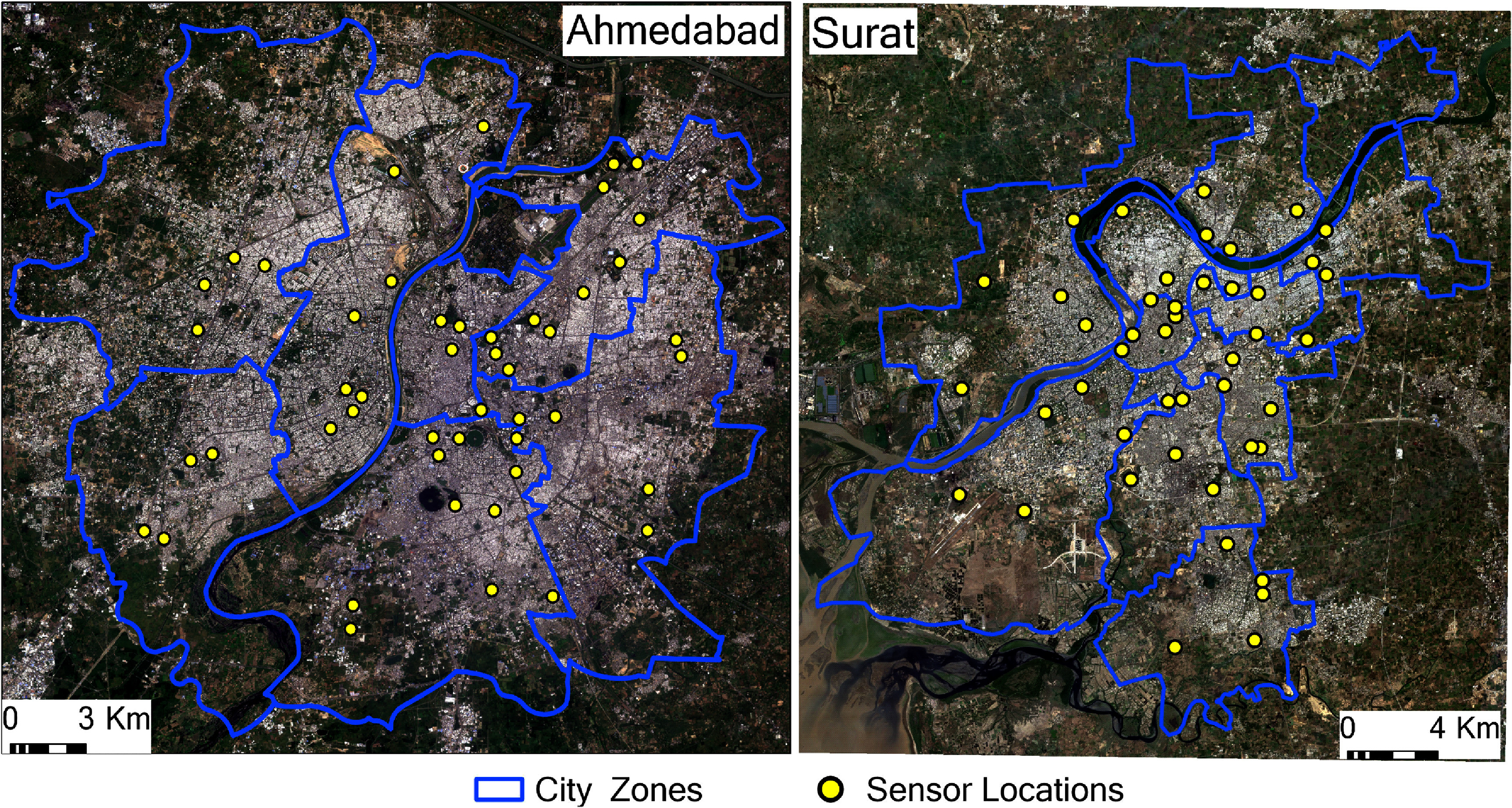 Figure 1
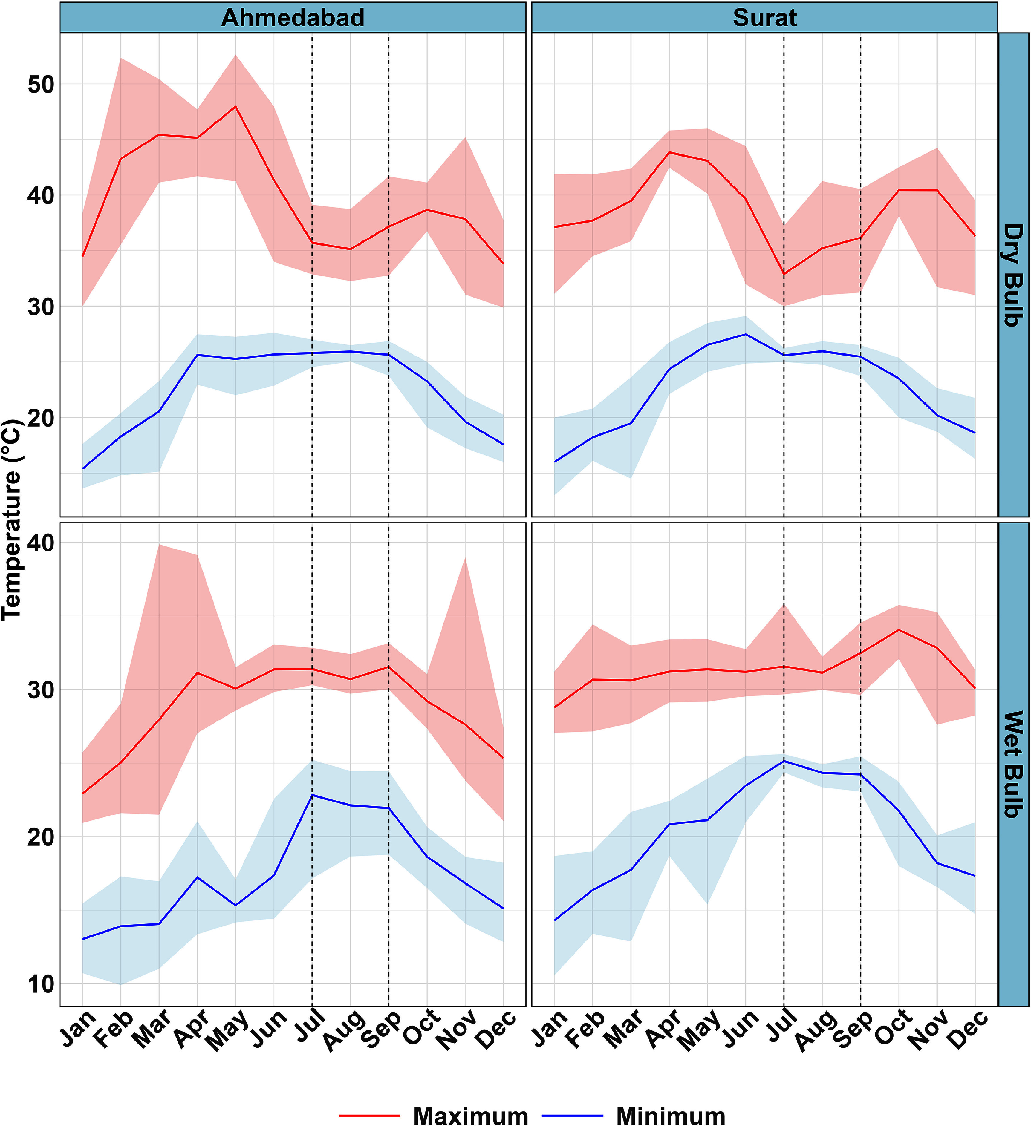 Figure 2
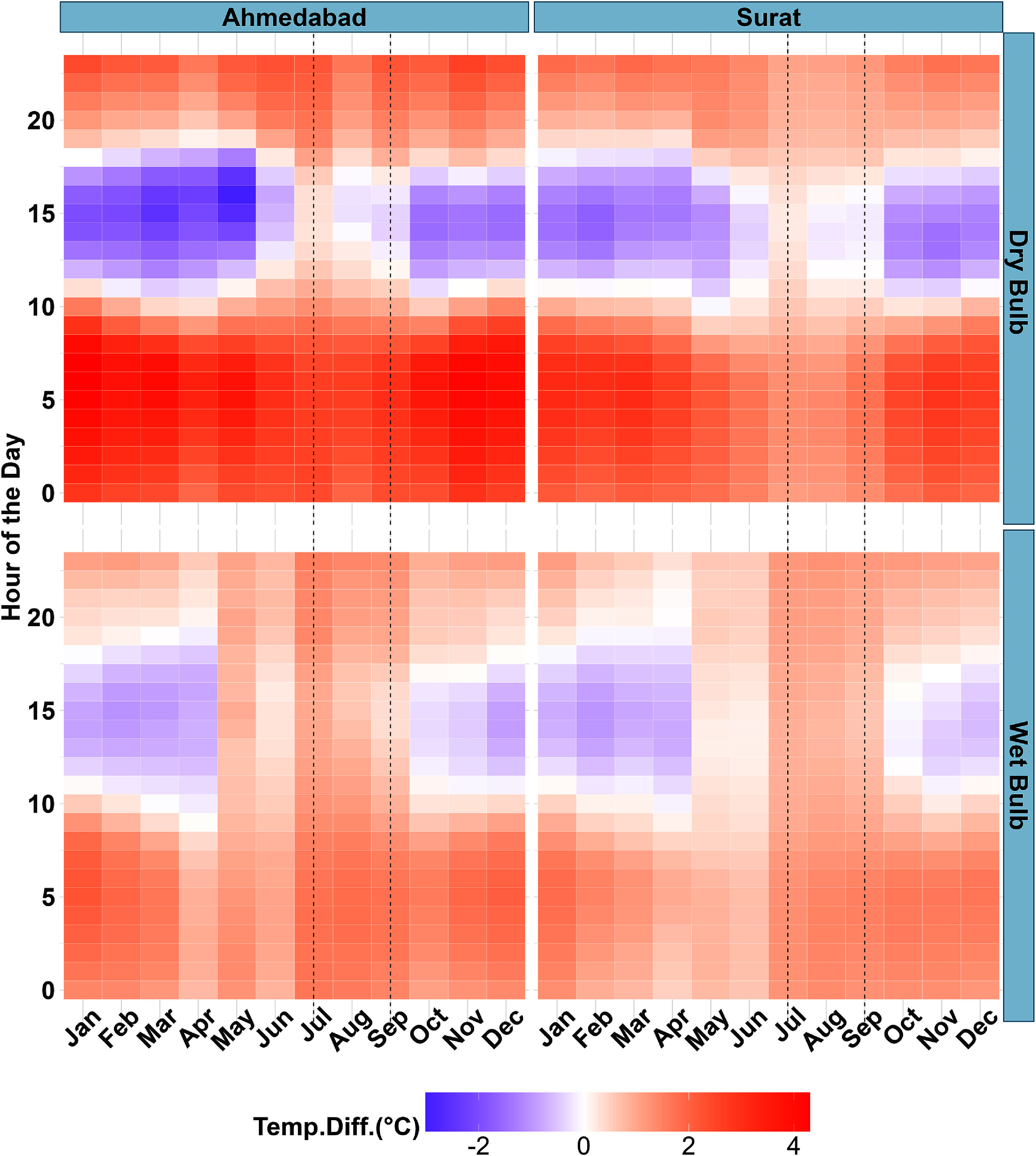 Figure 3
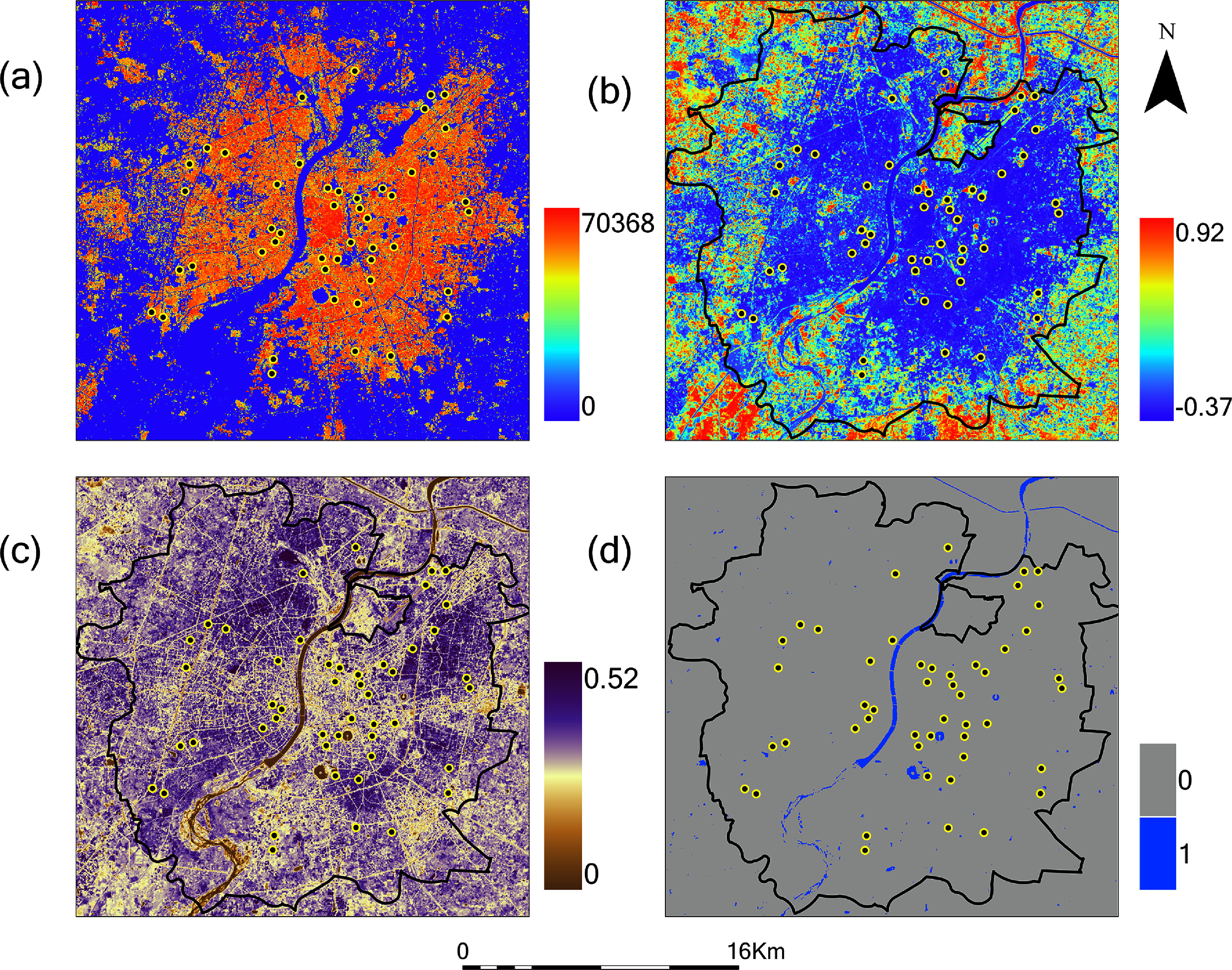 Figure 4
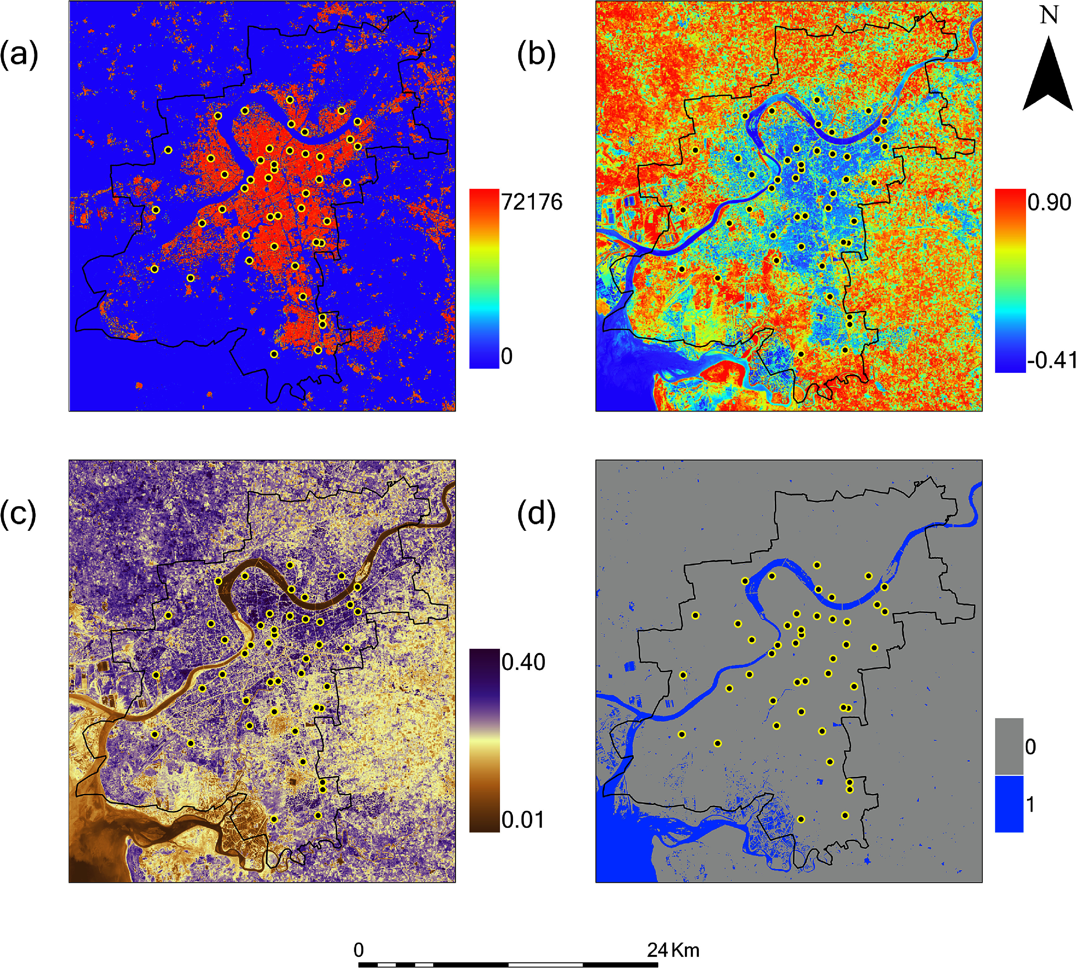 Figure 5
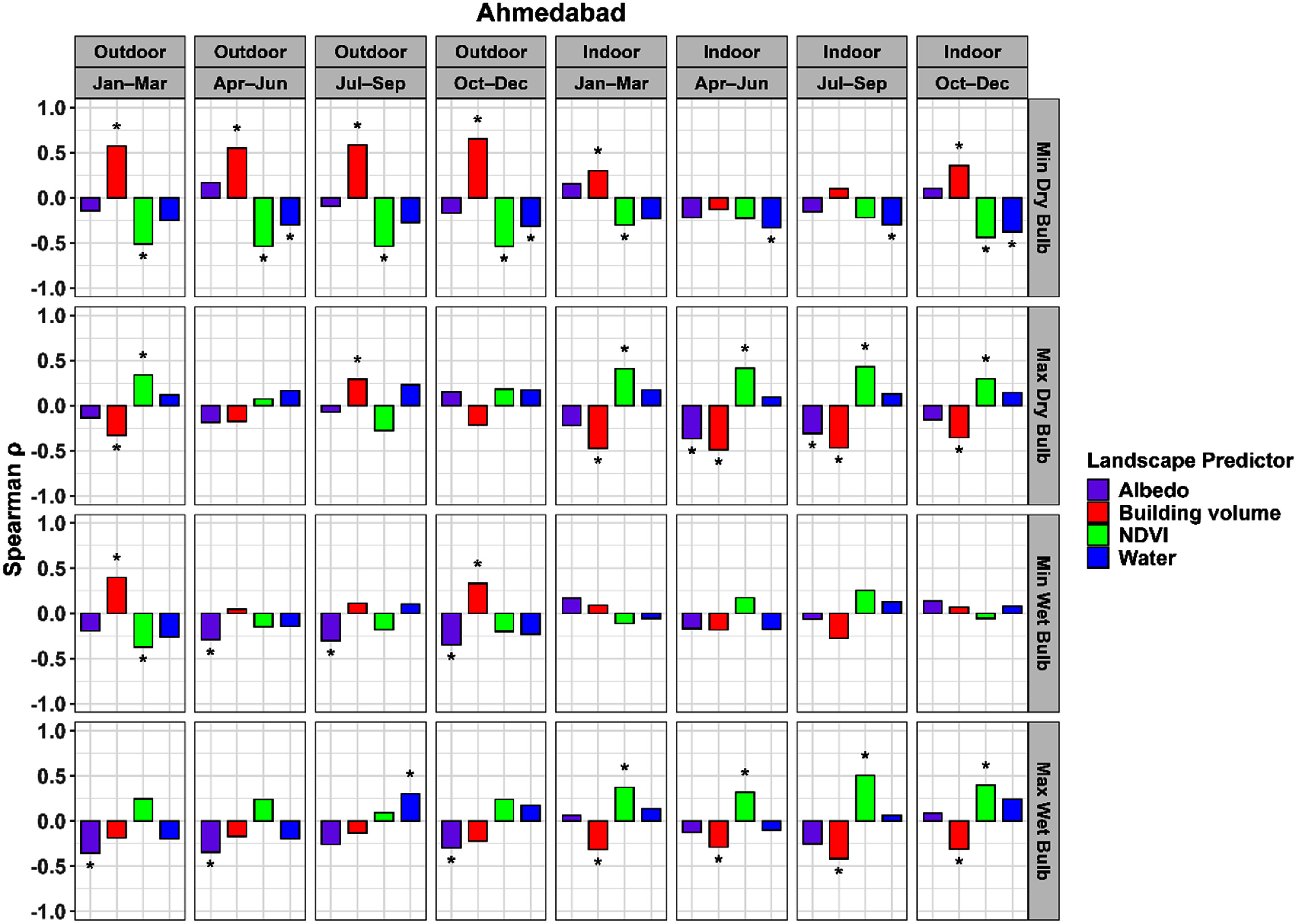 Figure 6
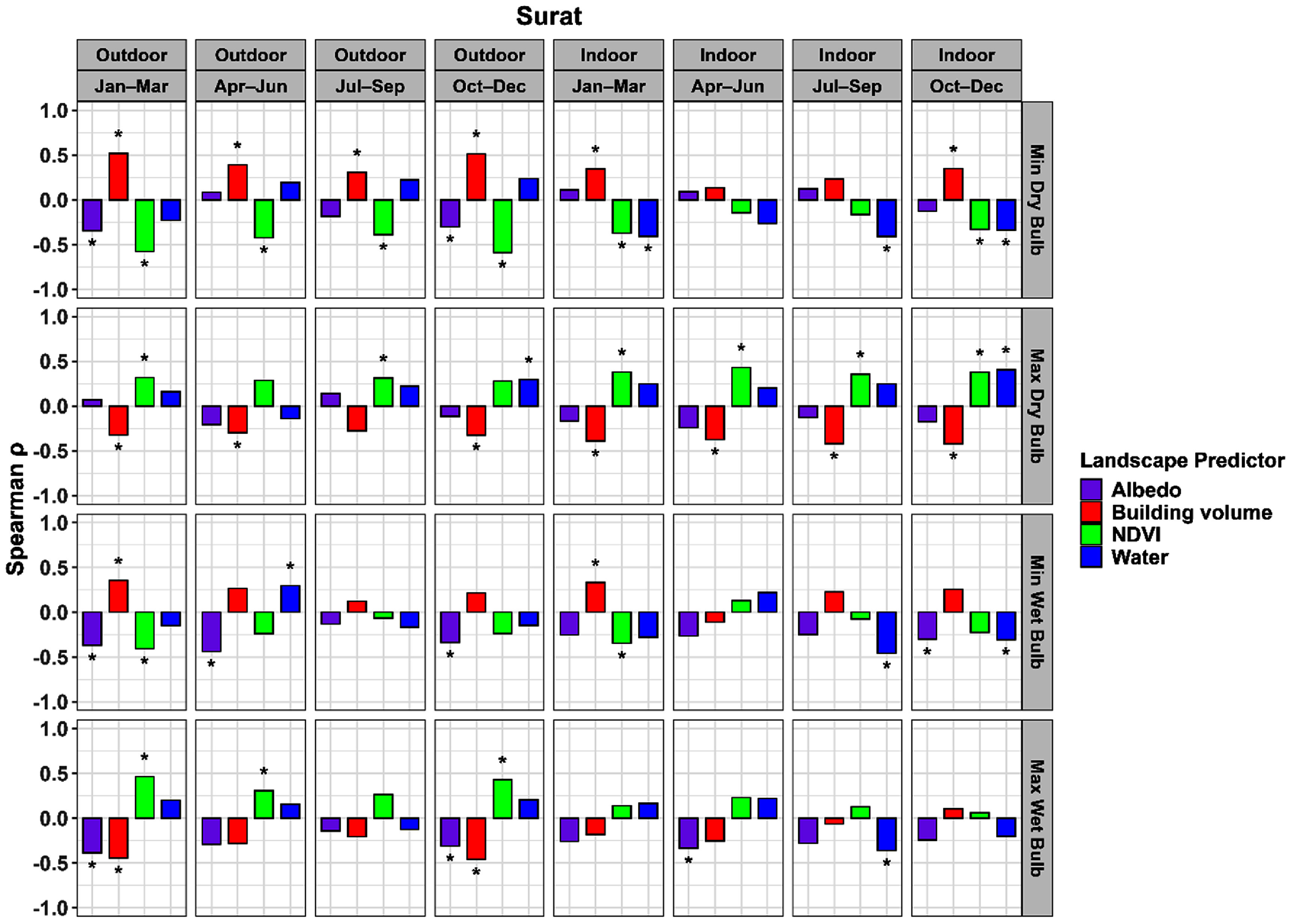 Figure 7
| Temperature variable | Model 1 | Model 2 | Change in AIC | |||
|---|---|---|---|---|---|---|
| Location |
| AIC |
| AIC | ||
|
| Surat | 0.70 | 3817 968 | 0.74 | 3696 508 | −121 460 |
|
| Ahmedabad | 0.65 | 3488 610 | 0.68 | 3422 873 | −65 737 |
|
| Surat | 0.78 | 3482 199 | 0.79 | 3447 554 | −34 645 |
|
| Ahmedabad | 0.69 | 3307 251 | 0.70 | 3283 705 | −23 546 |
| Temperature metric | Location | Model 3 | Model 4 | Change in AIC | ||
|---|---|---|---|---|---|---|
|
| AIC |
| AIC | |||
| Minimum | Ahmedabad | 0.66 | 1619.25 | 0.94 | 988.23 | −631.02 |
| Maximum | Ahmedabad | 0.71 | 1522.43 | 0.79 | 1417.65 | −104.78 |
| Minimum | Surat | 0.72 | 1332.55 | 0.89 | 1014.73 | −317.82 |
| Maximum | Surat | 0.59 | 1471.04 | 0.63 | 1449.57 | −21.47 |
| Temperature Metric | Location | Model 3 | Model 4 | Change in AIC | ||
|---|---|---|---|---|---|---|
|
| AIC |
| AIC | |||
| Minimum | Ahmedabad | 0.94 | 1042.04 | 0.97 | 769.52 | −272.52 |
| Maximum | Ahmedabad | 0.94 | 898.85 | 0.95 | 850.29 | −48.56 |
| Minimum | Surat | 0.93 | 897.72 | 0.96 | 731.00 | −166.72 |
| Maximum | Surat | 0.83 | 1030.56 | 0.86 | 979.15 | −51.41 |
- —National Institute of Allergy and Infectious Diseases10.13039/100000060
- —National Aeronautics and Space Administration10.13039/100000104
Peer Reviews
No public reviews on file for this paper yet. If you reviewed it on a platform where reviews are public (OpenReview, ICLR, NeurIPS, ICML), you can paste yours below so the community can read it here.
Videos
No videos yet. Explain this paper in a talk, walkthrough, or lecture? Add one.
Taxonomy
TopicsUrban Heat Island Mitigation
Introduction
Global temperatures are rising due to climate change, directly and indirectly affecting human health worldwide through various pathways (McMichael et al 2006). In addition to temperature, short-term and long-term variations of other climatological variables like humidity, wind speed, precipitation, and solar radiation have been reported to affect human health (Kinney 2008, Morin et al 2013). Most of the world’s population lives in cities, where microclimates are influenced by the built environment, other land cover characteristics such as water, vegetation and trees, and anthropogenic processes (Duarte et al 2015, Wong et al 2016, Yang et al 2023). These factors contribute to phenomena such as the urban heat island (UHI), dry island, and moist island effects that make weather in cities different from the surrounding rural areas (Wang and Gong 2010, Lokoshchenko 2017, Hao et al 2018, Shi and Zhang 2022). Although there is a large body of work in urban microclimatology, it is mostly focused on outdoor locations (Chatzidimitriou and Yannas 2015, Piselli et al 2018, Jacobs et al 2019). To improve our understanding of urban climate and health, there is a need to contrast these findings with studies of the indoor microenvironments where people spend much of their time.
Temperature, and its effects on health, can be characterized by different metrics. Dry-bulb temperature (T) refers to the ambient air temperature unaffected by the moisture of the air. T is the standard measurement of air temperature, indicating the heat content of the air. However, extreme heat impacts human health depending on humidity (Davis et al 2016). In particular, high humidity limits evaporative cooling, and increases the risk of heat stress and heat-related illnesses (Mitchell et al 1976, Cramer et al 2022). Wet bulb temperature (Tw), defined as the lowest temperature the air can reach through evaporative cooling, is thus an important metric for evaluating the physiological impacts of extreme heat (Justine et al 2023, Lu and Romps 2023). A threshold Tw of 35 °C has been proposed as the upper limit for human survivability, but other research suggests that this critical limit may be much lower under very hot and dry conditions (Vecellio et al 2022, Lu and Romps 2023). Therefore, it is essential to understand the spatial and temporal variability of T as well as Tw for assessment of human heat exposures. Previous studies have demonstrated that indoor and outdoor microclimates respond differently to surrounding built-up and landcover features (Liu et al 2022, Salvati et al 2022). In this context, distinguishing between indoor and outdoor environments is important, as they present considerably different heat exposure conditions (Quinn et al 2014).
In addition to direct heat impacts, variations in urban microclimates are also associated with indirect health effects such as habitat suitability for mosquitoes and transmission of mosquito-borne diseases (LaDeau et al 2015, Misslin et al 2016, Wimberly et al 2020). Because temperature and humidity exhibit local variations within cities, conventional weather station data cannot provide precise estimations of local exposures (Wimberly et al 2020, Ramsay et al 2021). Moreover, urban landscapes are inherently heterogeneous, encompassing variations in socio-economic conditions, vegetation cover, built density, and land use patterns as well as microclimate. Therefore, data that characterize the temporal (diurnal and seasonal) and spatial patterns of microclimate variables at the neighborhood scale are essential to assess climate-related health risks in urban neighborhoods.
Urban microclimates are influenced by land cover characteristics such as building volume, surface albedo, and vegetation cover (Bowler et al 2010, Kamal et al 2021, Smith et al 2023, Li et al 2024). Dense building volumes trap heat and limit ventilation, intensifying UHI effects, while high-albedo surfaces reflect sunlight, reducing local temperatures (Akbari et al 2001, Santamouris 2014). Vegetation reduces urban temperatures by providing shade, which blocks solar radiation, and through evapotranspiration, which releases water vapor to cool surrounding air (Qiu et al 2017, Venter et al 2020). Proximity to water bodies, such as rivers or lakes, moderates urban temperatures by slowly absorbing and releasing heat, creating a cold island effect and enhancing cooling through evaporation, improving thermal comfort in hot conditions (Hathway and Sharples 2012, Norton et al 2015).
Indoor microclimates are further influenced by the outdoor environment, but these effects are modulated by building materials, insulation, and ventilation systems (Erell and Zhou 2022). Numerous studies have explored these relationships in a wide range of urban environments (Andreou 2013, Priya and Senthil 2021, Salvati et al 2022, Zhang et al 2022). However, fewer studies have directly compared the spatial and temporal patterns of indoor and outdoor microclimates and their distinctive associations with urban land cover (Scott et al 2017, Asumadu-Sakyi et al 2019, Mukhopadhyay et al 2021, Salvati et al 2022). More research is needed to assess neighborhood-level microclimate variation at scales that are relevant to indoor and outdoor exposures and health risks in dense urban landscapes.
To address this gap, we installed a network of temperature/humidity sensors in Ahmedabad and Surat—two Indian cities—to capture fine-scale variation in temperature and atmospheric humidity. We also obtained satellite-derived estimates of building volume, surface albedo, vegetation indices, and proximity to water to understand their influence on the microclimate at varying spatial scales. The specific research questions were 1) how do indoor and outdoor air temperature (T) and wet bulb temperature (Tw) differ in their diurnal and seasonal variability across urban neighborhoods?, 2) how are indoor and outdoor T and Tw associated with land cover, including building volume, vegetation, surface albedo, and water?, and 3) do indoor and outdoor T and Tw exhibit significantly distinct temporal and spatial patterns, indicating differential sensitivity to environmental and land cover features?
Methods
Study area
2.1.
Our study area encompassed Ahmedabad and Surat, two major cities in Gujarat state, India. The cities have tropical climates characterized by a hot and dry season from March–June, a wet and humid monsoon season from July–September, and a cooler and drier post-monsoon season from October–February. Severe heat waves have impacted both cities in recent years, and the frequency of these events is projected to increase with climate change (Azhar et al 2014, Bandyopadhyay et al 2016, Im et al 2017). Despite their geographical proximity, the cities have different environmental and demographic characteristics.
Ahmedabad has a hot semi-arid climate, with average minimum and maximum temperatures of 26.3 °C and 41.4 °C during May and 13.1 °C and 28.7 °C during January. An average of three heatwave days was recorded each year during the March–May period from 2010 to 2016, including a peak temperature of 48 °C on 20 May 2016. Notably, the May 2010 heatwave resulted in a total of 1344 recorded deaths (Azhar et al 2014). Ahmedabad is slightly drier than Surat, with 782.2 mm of annual precipitation (WMO Climate Normals 2021). The city spans 466 sq. km and is projected to have a population of 8.16 million in 2025, with a density of 9900 persons per sq. km and an annual growth rate of 2.35% (Ahmedabad City Population | Literacy and Hindu Muslim Population 2025, Demography | Ahmedabad District, Government Of Gujarat | India 2025).
Surat, located along the Arabian Sea, has a tropical wet and dry climate, with average minimum and maximum temperatures of 26.3 °C and 36.2 °C during May and 14.7 °C and 30.9 °C during January. An average of seven heatwave days (defined as days with temperatures exceeding 40 °C) has been observed annually since 2010, with a peak of 22 such days recorded in 2010 (Magotra et al 2023). Total annual rainfall is approximately 1200 mm. (WMO Climate Normals 2021). Covering 462.1 sq. km, Surat has a population of 6.53 million in 2025, with a density of 10 052 persons per sq. km (2011 census) and an annual growth rate of 3.1% (Surat Municipal Corporation 2025, Surat City Population | Literacy and Hindu Muslim Population 2025).
Data collection and pre-processing
2.2.
Microclimate data
2.2.1.
Microclimate monitoring networks were established in both cities with Monarch Instruments Track-It temperature/humidity sensors collecting data on dry-bulb temperature (T) and relative humidity (RH) every 10 sec, which were then averaged and recorded every 30 min from 1 May 2023 through 30 April 2024. They were installed at paired indoor/outdoor locations in 48 houses in Ahmedabad and 45 houses in Surat (figure 1). These houses were involved in the vector surveillance programs in each city and were geographically stratified by administrative zone (six sensors in each of eight zones in Ahmedabad and five sensors in each of nine zones in Surat). Sensors were positioned to avoid direct sunlight and proximity to heat- or cold-emitting devices or surfaces. Indoor sensors were placed on walls of living or sleeping rooms with no air conditioners, and outdoor sensors were placed in locations near dwellings with shade from porch roofs or vegetation. Measurements were taken every half hour for a full year. Data were downloaded monthly by vector surveillance personnel using an Android mobile phone app and submitted by email for processing and analysis.
Sensor locations in Ahmedabad and Surat. There is one indoor and one outdoor sensor at each dwelling. Points are jittered to anonymize dwelling locations. Background imagery is from PlanetScope dated 5 October 2023, for Ahmedabad and 25 February 2024, for Surat (Imagery © 2024 Planet Labs Inc.).
The time series of T and RH obtained from loggers were summarized as mean hourly observations. An algorithm was developed to fill data gaps (8.3% of observations in Ahmedabad and 2.2% in Surat) using data collected from other loggers during the gap periods. We imputed missing data in these gaps using time series models calibrated using data from other sensors. More details on data imputation are provided in section 1 of supplementary information. Wet bulb temperature (Tw) was calculated as a function of T and Tw using an empirical relationship (Stull 2011).
Satellite remote sensing data
2.2.2.
Building volume was obtained by combining 2023 data from Google Buildings 2.5D Temporal V1-4 m rasters from Sentinel-2 imagery with building height information and Google Open Buildings V3-Polygons from very high resolution imagery (Open Buildings 2.5D Temporal Dataset 2025, Open Buildings Temporal V1 | Earth Engine Data Catalog 2025). The resulting building volume raster had a 30 m grid cell size. Harmonized Landsat and Sentinel-2 (HLS) images were obtained for Ahmedabad and Surat from May 2023 to April 2024, summarized as median monthly composites, and used to derive the normalized difference vegetation index (NDVI) (Claverie et al 2018). Broadband albedo was estimated from spectral bands of HLS images using Liang’s equation (Liang 2001). We computed the modified normalized difference water index (MNDWI) from HLS spectral bands and applied a threshold of 0.05 to effectively distinguish water from non-water regions (Xu 2006). Based on this threshold, we created a binary raster mask, assigning a value of 1 to pixels with MNDWI values greater than 0.05 (indicating water presence) and 0 otherwise (indicating absence of water). Procedures for building volume estimation and processing of HLS images are detailed in section 2 of the supplementary information (Jamal et al 2025).
Analysis
2.3.
Seasonal and diurnal patterns of minimum and maximum T and Tw were assessed by graphing the time series of monthly values and summarizing the mean differences between paired indoor and outdoor loggers by month and time of day. Spatial patterns were assessed by computing the correlations between microclimate variables (minimum and maximum T and Tw) and land cover variables (building volume, NDVI, broadband albedo, and surface water). Each variable was summarized at four focal window sizes (50 m, 100 m, 500 m, and 1000 m) around each microclimate sensor to capture effects from immediate surroundings up to neighborhood-scale influences. Monthly data for all microclimate variables and predictors were averaged seasonally, using four seasons: cold dry (January–March), hot dry (April–June), monsoon (July–September), and wet (October–December).
We calculated Spearman rank correlations to quantify the strength and direction of associations between each microclimate variable and predictor for each season and indoor versus outdoor locations. For each combination of microclimate and land cover variable, we calculated the absolute Spearman correlation for different window sizes, then averaged these values across all seasons and both indoor and outdoor locations to obtain average absolute correlation (|ρ|). The spatial window with the highest average absolute correlation was used to model the relationship between that specific temperature–predictor. The spatial windows with the highest |ρ| are explained in section 3.1 of the supplementary information.
We used generalized additive models to assess whether temporal microclimate patterns and spatial associations with land cover were distinctive at indoor versus outdoor locations. For the temporal trend models (Model 1 and Model 2), the response variables were hourly T and Tw and the predictor variables were a tensor product of hour of day and month. The tensor product function allowed interaction effects between the two predictor variables. In Model 2, the smoothed function differed with indoor versus outdoor location,
\documentclass[12pt]{minimal} \usepackage{amsmath} \usepackage{wasysym} \usepackage{amsfonts} \usepackage{amssymb} \usepackage{amsbsy} \usepackage{upgreek} \usepackage{mathrsfs} \setlength{\oddsidemargin}{-69pt} \begin{document} \begin{equation*}{\boldsymbol{Model}}1:{\text{Temp}}\sim te\left( {{\text{Hour}}\;{\text{of}}\;{\text{Day,Day}}\;{\text{of}}\;{\text{year}}} \right) + \epsilon \end{equation*}\end{document} \documentclass[12pt]{minimal} \usepackage{amsmath} \usepackage{wasysym} \usepackage{amsfonts} \usepackage{amssymb} \usepackage{amsbsy} \usepackage{upgreek} \usepackage{mathrsfs} \setlength{\oddsidemargin}{-69pt} \begin{document} \begin{align*} & {\boldsymbol{Model}}\,2:{\text{Temp}} \nonumber\\ & \quad \sim te{\text{(Hour}}\;{\text{of}}\;{\text{Day,Day}}\;{\text{of}}\;{\text{year|}}{\text{Location}}) + \epsilon .\end{align*}\end{document}For the spatial trend models (Model 3 and Model 4), the response variables were seasonal minimum and maximum T and Tw the predictor variables included additive smooth terms represented by thin plate regression splines for albedo, building volume, NDVI, and surface water presence, along with season as a categorical predictor. In Model 4, the smoothed functions and the seasonal variable differed with indoor versus outdoor location. The land cover variables were summarized at their respective optimal focal windows as described earlier in this section,
\documentclass[12pt]{minimal} \usepackage{amsmath} \usepackage{wasysym} \usepackage{amsfonts} \usepackage{amssymb} \usepackage{amsbsy} \usepackage{upgreek} \usepackage{mathrsfs} \setlength{\oddsidemargin}{-69pt} \begin{document} \begin{align*} & {\boldsymbol{Model}}\,3:{\text{Temp}}. \sim s\left( {{\text{albedo}}} \right) + s\left( {{\text{buildingvolume}}} \right) \nonumber\\ & \quad + s\left( {{\text{NDVI}}} \right) + s\left( {{\text{water}}} \right) + {\text{Season}} + \epsilon \end{align*}\end{document} \documentclass[12pt]{minimal} \usepackage{amsmath} \usepackage{wasysym} \usepackage{amsfonts} \usepackage{amssymb} \usepackage{amsbsy} \usepackage{upgreek} \usepackage{mathrsfs} \setlength{\oddsidemargin}{-69pt} \begin{document} \begin{align*} & {\boldsymbol{\,Model}}\,4:{\text{Temp}}. \sim {{s}}\left( {{\text{albedo|Location}}} \right) \nonumber\\ & \quad + s\left( {{\text{buildingvolume|Location}}} \right) \nonumber\\ & \quad + s\left( {{\text{NDVI|Location}}} \right) \nonumber\\ & \quad + s\left( {{\text{water|Location}}} \right) \nonumber\\ & \quad + {\text{Season}}|{\text{Location}} + \epsilon .\end{align*}\end{document}Models were fitted separately for Ahmedabad and Surat. Because building volume and NDVI were strongly correlated, we repeated the analysis without NDVI predictor to assess whether the results were sensitive to concurvity. Model performance and fit were evaluated and compared using the adjusted coefficient of determination (adjusted R^2^) and the Akaike information criterion (AIC). Higher adjusted R^2^ values indicated better explanatory power, while lower AIC values signified improved model parsimony and fit.
Results
Temporal patterns of microclimate variables
3.1.
Marked differences were observed between the monthly variations of T and Tw (figure 2). While maximum T values were generally lowest during the monsoon, maximum Tw values tended to peak during this season. However, the behavior of maximum Tw during and around the monsoon did not vary as sharply as that of maximum T. The monsoon had less effect on minimum T, whereas minimum Tw showed sharper peaks during the monsoon.
Monthly seasonality of dry and wet bulb temperatures with indoor and outdoor locations combined. May–December data are from 2023, and January–April data are from 2024. Shaded areas encompass 5%–95% quantiles. The duration between vertical dotted lines represents the monsoon season (July–September).
Diurnal and monthly variations were evident when differences between paired indoor and outdoor loggers were considered (figure 3). A consistent pattern emerged in which indoor temperatures were warmer than outdoor temperatures from sunset until approximately 10 a.m. This temperature difference was less pronounced for Tw compared to T. This pattern reversed from around 10 a.m. to 6 p.m., when outdoor temperatures became warmer than indoor temperatures. After 6 p.m., indoor temperatures again became warmer, although the magnitude of this difference decreased compared to morning. However, this reversal pattern was not as evident during the monsoon season, as the differences between indoor and outdoor temperatures became minimal between noon (12 p.m.) and 6 p.m. The reversal effect was not observed for Tw during the monsoon.
Difference between indoor and outdoor temperatures (indoor–outdoor) by month and hour of the day. May–December data are from 2023, and January–April data are from 2024. The months between vertical dotted lines represent the monsoon season (July–September).
Correlations between microclimate variables and landscape metrics
3.2.
There was decreasing building volume and increasing NDVI along a gradient from the city center to the periphery in both Ahmedabad (figure 4) and Surat (figure 5). As a result, building volume and NDVI at the sensor locations was strongly correlated (Spearman correlation −0.80 to −0.83 for Ahmedabad, and −0.78 to −0.80 for Surat when both variables were summarized with a focal window of 100 m). Patterns of albedo captured finer-scale variation in the reflective properties of buildings, vegetation and soil. Water reflected the central river bisecting each city as well as smaller ponds for water storage, recreation, and aquaculture.
Satellite-derived measurements of land cover for Ahmedabad-(a) building volume (in m3 per 30 m grid cell), (b) vegetation (NDVI) for October 2023, (c) surface reflectivity (albedo) for October 2023, and (d) water presence for October 2023 (MNDWI for water presence,1 indicates MNDWI > 0.05, 0 indicates MNDWI < 0.05). Black line represents Ahmedabad city boundary. Black dots with yellow outline represent sensor locations inside Ahmedabad city.
Satellite-derived measurements of land cover for Surat-(a) building volume (in m3 per 30 m grid cell), (b) vegetation (NDVI) for October 2023, (c) surface reflectivity (albedo) for October 2023, and (d) water presence for October 2023 (MNDWI for water presence,1 indicates MNDWI > 0.05, 0 indicates MNDWI < 0.05). Black line represents Surat city boundary. Black dots with yellow outline represent sensor locations inside Surat city.
The focal window size with the highest mean absolute correlation was determined for each combination of city, land cover variable, and temperature variable (T or Tw). The correlations for these windows are shown in figure 6 for Ahmedabad and figure 7 for Surat. Correlations for all window sizes and optimal window sizes are shown in section 3 of the supplementary information (figures S3–S11).
Spearman correlations between microclimate variables and predictors for Ahmedabad. The stars above (or below) the bars show statistical significance at an alpha level of 0.05.
Spearman correlations between microclimate variables and predictors for Surat. The stars above (or below) the bars show statistical significance at an alpha level of 0.05.
Among the four land cover variables, building volume showed the most consistent correlation patterns across both Ahmedabad (figure 6) and Surat (figure 7). Correlations were generally stronger in outdoor settings than indoors, especially for minimum T and Tw. Outdoor minimum T had the highest positive correlations across all seasons, while indoor minimum T also displayed significant but lower positive correlations, particularly during January–March and October–December. In contrast, maximum T and Tw tended to have negative associations with building volumes. Overall, correlations were stronger and more significant for T than Tw.
Compared to building volume, NDVI exhibited inverse patterns of association with T and Tw and across both cities. Correlations were generally stronger in outdoor environments, particularly for minimum T and Tw, where NDVI showed consistent negative relationships across seasons. The highest outdoor correlations were observed with minimum T and Tw. Indoor correlations were lower with less seasonal consistency. For maximum T and Tw, NDVI exhibited significant positive associations both indoors and outdoors.
It is notable that indoor maximum T was negatively correlated with building volume and positively correlated with NDVI, a pattern that contrasted with the expected cooling effect of vegetation. The observed effects were consistent across both cities for indoor temperature, and similar associations were also observed outdoors, although with fewer significant relationships. In Ahmedabad, maximum Tw also exhibited stronger correlations indoors, but weaker and insignificant correlations outdoors. In Surat, maximum Tw exhibited stronger correlations outdoors compared to indoors.
Albedo showed consistently negative relationships with T and Tw. These associations displayed less variation across indoor and outdoor settings compared to building volume and NDVI. Notably, outdoor Tw had higher correlations with albedo than outdoor T, particularly in Ahmedabad.
Water presence, represented by masked MNDWI, had some significant correlations at the largest spatial window of 1000 m. Consistent negative correlations were observed for indoor and outdoor minimum T across both cities. Correlations with other temperature variables were generally lower and more variable. In Surat, water exhibited stronger and more statistically significant correlations with Tw than Ahmedabad.
Modeling the influence of location in the spatial and temporal variation of microclimate variables
3.3.
Modeling temporal variation
3.3.1.
The models explained substantial portions of the temperature variation (table 1). In both cities, higher adjusted R^2^ values and lower AIC values were observed for Model 2 for T and Tw, indicating distinctive patterns of diurnal and seasonal variation at indoor versus outdoor locations. The adjusted R^2^ values were all slightly higher for Surat than Ahmedabad, indicating that the diurnal and season trends were stronger and explained more of the variation in T and Tw.
Modeling spatial variation
3.3.2.
In both Ahmedabad (table 2) and Surat (table 3), Model 4 consistently outperformed Model 3 across all temperature metrics (minimum and maximum T and Tw). Model 4 achieved consistently higher R^2^ values and lower AIC values, indicating better model fit when land cover associations were allowed to vary across indoor versus outdoor locations. The differences were most pronounced for minimum T and Tw in both cities, with substantial AIC reductions. All differences between Model 3 and Model 4 were statistically significant (ANOVA, p < 0.05). Similar results were obtained after fitting models 3A and 4A, which excluded NDVI as a predictor (tables 2(A) and 3(A) in section 4 of the supplementary information, demonstrating that the correlation between NDVI and building volume did not bias our conclusions.
Discussion
Our findings show that building volume was positively correlated with minimum nighttime T, with stronger relationships outdoors, highlighting an UHI effect driven by heat retention in densely built areas (Santamouris 2014, Hsu et al 2021). Vegetation, quantified via NDVI, was negatively associated with nighttime T, particularly outdoors, as areas with high NDVI typically correspond to lower building volume and reduced impervious surface coverage, allowing them to cool more efficiently at night due to lower thermal inertia (Bowler et al 2010, Meili et al 2021). Weaker indoor correlations with both building volume and NDVI suggest that the insulating effects of structures moderate temperature extremes (Qiu et al 2017, Salvati et al 2022). These results generally agree with previous studies in a variety of cities that have found that measures of urbanization density are typically associated with higher minimum dry-bulb temperature (Oleson et al 2015, Chapman et al 2017, Logan et al 2020). Correlations between building volume and minimum Tw had similar patterns but were weaker, indicating that moist heat stress, is sensitive to other factors that constrain the patterns.
Maximum T was also associated with building volume and NDVI. In contrast to minimum T, the correlations were reversed, so that maximum T at both indoor and outdoor locations was warmest in areas with low building volume and high NDVI. Because of the underlying negative correlation between building density and NDVI, this effect reflected an urban to rural gradient with lowest maximum T in the densely developed urban core and the highest maximum T at more isolated dwellings near the urban periphery. These findings contrast with the general expectation that daytime temperature, including land surface temperature as well as air temperature, will be lowest in vegetated areas because of cooling effects of evapotranspiration and shade (Mildrexler et al 2011, Napoli et al 2016, Qiu et al 2017). As with minimum temperature, these patterns are generally consistent between T and Tw, although there are fewer statistically significant correlations with Tw.
Previous studies have demonstrated that urban morphology has a significant influence on indoor thermal environments (Robinson 2006, Mirzaei et al 2012). A modeling study conducted in urban Singapore concluded that increased building density can reduce indoor temperatures during daytime, primarily due to the shielding effect, whereby closely spaced buildings block direct solar radiation and thus reduce indoor heat gain (Li et al 2022). Furthermore, the influence of building density on indoor air temperatures tends to be more pronounced during the day than at night, when solar exposure is minimal (Mills 1997). On the other hand, locations characterized by lower building density and higher NDVI generally have a higher sky view factor, which has been linked to elevated indoor temperatures during daytime due to greater exposure to direct solar radiation (Zheng and Li 2022).
The results for maximum temperature should be interpreted in the context of our microclimate sampling design. Sensors were located at individual dwellings, which ranged from ground-floor apartments in the urban core to blocks of detached houses in outlying neighborhoods to more isolated dwellings at the urban fringe. Outdoor sensors were placed on or near and exterior wall of a house, typically in a shaded area on a porch. Thus, the outdoor temperatures represent microclimates in close proximity to buildings and may be sensitive to similar insulating effects as indoor temperatures during the day. Also, vegetation cover within these cities was generally low, and our sampling design did not incorporate locations close to parks or other places with urban vegetation densities. Thus, our finding of higher temperatures in locations with higher NDVI does not mean that vegetation cooling is not occurring in other areas, but it does suggest that cooling effects related to building density are more important in some indoor locations and outdoor spaces proximal to those buildings.
Surface albedo exhibited significant negative correlations with temperature, most commonly for Tw and at outdoor locations, indicating that more reflective buildings tended to have lower temperatures. High-albedo materials reflect a greater portion of incoming solar radiation, thereby reducing heat absorption at the surface. This negative association supports the concept of cool roofs, designed to mitigate urban heat (Sharma et al 2016, Wang et al 2022). However, these albedo effects are contingent on a variety of other factors including urban canyon effects, multiple reflections and shadowing (Akbari et al 2001, Chatzidimitriou and Yannas 2015). There were some negative correlations observed between minimum T and water presence at 1000 m spatial scale and these likely reflect the cold island effect produced by rivers (He et al 2024). Additionally, the urban morphology surrounding rivers and the configuration of adjacent green spaces can influence the strength of the cold island effect, potentially explaining the differing behaviors observed between Ahmedabad and Surat (Saaroni and Ziv 2003, Wang and Chen 2025).
Tw showed different associations with landscape predictors than T because Tw depends on atmospheric humidity in addition to air temperature. The effects of land cover on humidity are different from effects on temperature, reflecting local inputs sources from evapotranspiration combined with dynamic mixing of air (Findell et al 2017, Rahman et al 2022, Zhang et al 2023, Chagnaud et al 2025). For example, the negative correlations that we observed between albedo and Tw may reflect reduced evapotranspiration and humidity in areas with dense buildings and concrete surfaces in addition to reflectance of incoming solar radiation. Because of the combined physical mechanisms through which surface energy and moisture exchange processes affect temperature and humidity, land cover relationships are complex and represent an important area for further research.
Many previous studies comparing indoor and outdoor urban microenvironments lacked a spatially representative distribution of sensors across the study area, such as sensor placements that were clustered in specific parts of the city rather than being spread across the urban-to-rural gradient. In addition, many studies only collected data for short periods, ranging from a few days or a month, which is not enough to capture seasonal microclimate patterns (Nguyen and Dockery 2016, Moghbel and Erfanian Salim 2017, Tasgaonkar et al 2022). In contrast, our study stratified sensors across zones within each city and covers a full year of data collection, enabling detailed exploration of spatiotemporal trends. Moreover, our methodology of pairing indoor and outdoor sensors provides precise estimations of the differences in microenvironmental conditions at each dwelling.
Our study expands upon previous work focused on T by additionally considering diurnal and spatial variations in Tw, thus demonstrating broader insights. Compared to T, fewer studies have studied spatiotemporal variation in Tw, specifically in the context of assessing indoor heat stress (Gaspar and Quintela 2009, Hall et al 2022). Previous interpretations of Tw have focused on threshold values of human thermal comfort (Epstein and Moran 2006, Abdel-Ghany et al 2013, Vecellio et al 2022). In Ahmedabad and Surat, Tw exhibits stronger diurnal and seasonal variation patterns than T, and land cover associations with Tw are distinctive from those with T. These observations have implications in tropical regions where air conditioning is uncommon (Amaripadath et al 2023).
Without adequately accounting for humidity, the extent and magnitude of heat stress exposure, especially in informal settlements, could be significantly underestimated (Mukhopadhyay et al 2021). Understanding indoor humidity patterns is particularly important because Tw directly affects the body’s ability to cool through sweating, and high Tw indoors can increase heat stress for vulnerable groups who spend most of their time inside (Vecellio et al 2022). During the pre-monsoon season, high temperatures combined with poor ventilation can create dangerously warm indoor conditions at night, limiting recovery from daytime heat (Sampson et al 2013, Hampo et al 2024). In the monsoon season, even when outdoor temperatures fall, persistently high Tw indoors reduces evaporative cooling, intensifying health risks (Ambika et al 2024, Masuda et al 2024).
This study focused on contrasting temperature in indoor versus outdoor environments in the context of diurnal and season trends and land cover effects on spatial patterns. Because remotely sensed land cover data are spatially contiguous and widely accessible, they are important for understanding and predicting the spatial patterns of urban heat (Rotem-Mindali et al 2015, Coutts et al 2016, Bonafoni et al 2017). Our results emphasize that indoor and outdoor temperatures have different land cover associations, and additional sources of information will be needed to better understand and predict these indoor patterns. Adaptive human behaviors such as the use of fans, window shutters, or sleeping positions all have the potential to mitigate indoor heat. Additionally, local data on building materials, and socioeconomic characteristics can help to explain more of the spatial variability in urban microclimates. Collection of these additional data sources can support more nuanced understanding of the proximal drivers influencing spatial variations in urban microclimate and provide a foundation for high-resolution predictive modeling of urban microclimate (Buyantuyev and Wu 2010, Wong et al 2016, Deng et al 2024).
Conclusions
Our findings demonstrate that it is important to distinguish between indoor and outdoor locations when studying the effects of urban land cover on dry and wet-bulb temperatures. In particular, we found that maximum indoor temperatures were coolest in neighborhoods with high building volume and low vegetation cover, running counter to the general expectation that urban vegetation will have a cooling effect. These insights are important for future efforts at predictive modeling of microclimate based on land cover and can inform urban planning and design strategies to mitigate heat and humidity, improving public health outcomes in tropical cities.
The reference list from the paper itself. Each links out to its DOI / PubMed record.
- 1Abdel-Ghany A M Al-Helal I M Shady M R 2013 Human thermal comfort and heat stress in an outdoor urban arid environment: a case study Adv. Meteorol.2013171–710.1155/2013/693541 · doi ↗
- 2Ahmedabad City Population 2025 | Literacy and Hindu Muslim Population 2025 Ahmedabad City Population 2025(available at: www.census 2011.co.in/census/city/314-ahmedabad.html)(Accessed 10 March 2025)
- 3Akbari H Pomerantz M Taha H 2001 Cool surfaces and shade trees to reduce energy use and improve air quality in urban areas Sol. Energy 70295310295–31010.1016/s 0038-092x(00)00089-x · doi ↗
- 4Amaripadath D Rahif R Velickovic M Attia S 2023 A systematic review on role of humidity as an indoor thermal comfort parameter in humid climates J. Build. Eng.6810603910.1016/j.jobe.2023.106039 · doi ↗
- 5Ambika A K Rajeev A Huber M 2024 Global warming amplifies outdoor extreme moist heat during the Indian summer monsoon Earth’s Future 12e 2024 EF 00467310.1029/2024 EF 004673 · doi ↗
- 6Andreou E 2013 Thermal comfort in outdoor spaces and urban canyon microclimate Renew. Energy 551828182–810.1016/j.renene.2012.12.040 · doi ↗
- 7Asumadu-Sakyi A B Barnett A G Thai P Jayaratne E R Miller W Thompson M H Roghani R Morawska L 2019 The relationship between indoor and outdoor temperature in warm and cool seasons in houses in Brisbane, Australia Energy Build.19112742127–4210.1016/j.enbuild.2019.03.010 · doi ↗
- 8Azhar G S Mavalankar D Nori-Sarma A Rajiva A Dutta P Jaiswal A Sheffield P Knowlton K Hess J J 2014 Heat-related mortality in India: excess all-cause mortality associated with the 2010 Ahmedabad heat wave P Lo S One on behalf of the Ahmedabad Heat Climate Study Group 9e 9183110.1371/journal.pone.009183124633076 PMC 3954798 · doi ↗ · pubmed ↗