Modeling the Role of Baseline Risk and Additional Study‐Level Covariates in Meta‐Analysis of Treatment Effects
Phuc T. Tran, Annamaria Guolo

TL;DR
This paper introduces a new method for meta-analysis that accounts for baseline risk and study-specific covariates to better understand treatment effect heterogeneity.
Contribution
The paper extends meta-analysis by incorporating additional covariates and correcting for measurement errors in baseline risk proxies.
Findings
The proposed method improves the reliability of meta-analysis by correcting for measurement errors in covariates.
Simulation studies show the method performs well under various conditions of sample size and heterogeneity.
The method was successfully applied to a meta-analysis on the association between COVID-19 and schizophrenia.
Abstract
The relationship between the treatment effect and the baseline risk is a recognized tool to investigate the heterogeneity of treatment effects in meta‐analyses of clinical trials. Since the baseline risk is difficult to measure, a proxy is adopted, which is based on the rate of events for the subject under the control condition. The use of the proxy in terms of aggregated information at the study level implies that the data are affected by measurement errors, a problem that the literature has explored and addressed in recent years. This paper proposes an extension of the classical meta‐analysis with baseline risk information, which includes additional study‐specific covariates other than the rate of events to explain heterogeneity. Likelihood‐based inference is carried out by including measurement error correction techniques necessary to prevent unreliable inference due to the…
Genes, proteins, chemicals, diseases, species, mutations and cell lines named across the full text — each resolved to its canonical identifier and authoritative record.
Click any figure to enlarge with its caption.
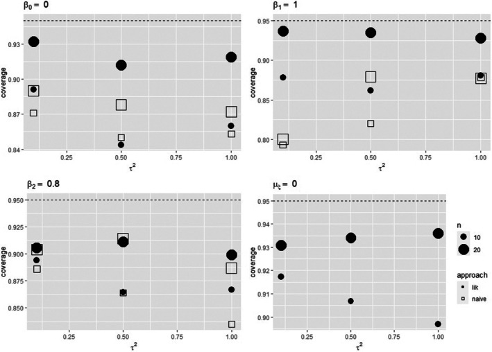 FIGURE 1
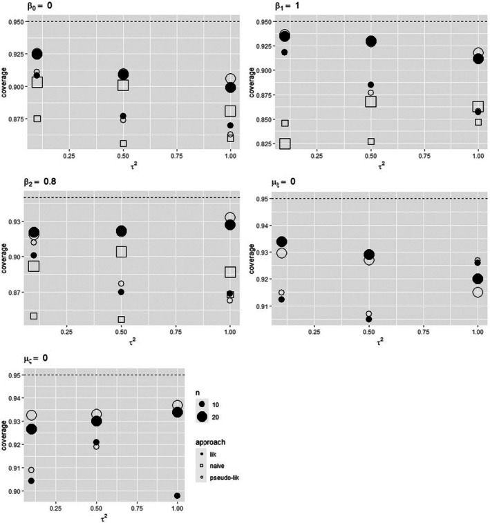 FIGURE 2
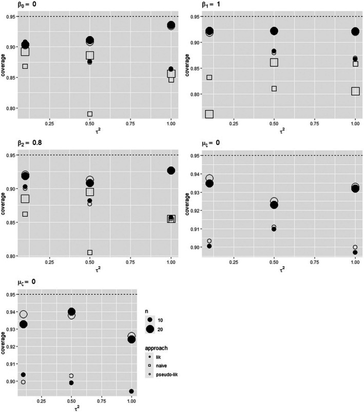 FIGURE 3
| Treatment group | Control group | ||||||
|---|---|---|---|---|---|---|---|
| Event | Non‐event | Event | Non‐event | ||||
| Male | Female | Male | Female | Male | Female | Male | Female |
| Treatment group | Control group | ||
|---|---|---|---|
| Event | Non‐event | Event | Non‐event |
| Parameter | Approach | bias | se | sd | convergence | bias | se | sd | convergence | |
|---|---|---|---|---|---|---|---|---|---|---|
| 0.1 | lik | 0.007 | 0.134 | 0.160 | 991 | −0.006 | 0.096 | 0.102 | 998 | |
| naive | 0.019 | 0.149 | 0.176 | 1000 | −0.003 | 0.104 | 0.121 | 1000 | ||
| lik | 0.011 | 0.172 | 0.214 | 991 | 0.012 | 0.121 | 0.136 | 998 | ||
| naive | −0.032 | 0.164 | 0.227 | 1000 | −0.061 | 0.107 | 0.147 | 1000 | ||
| lik | −0.014 | 0.134 | 0.160 | 991 | −0.010 | 0.119 | 0.128 | 998 | ||
| naive | 0.014 | 0.152 | 0.180 | 1000 | 0.014 | 0.140 | 0.157 | 1000 | ||
| lik | −0.010 | 0.302 | 0.314 | 991 | 0.016 | 0.219 | 0.224 | 998 | ||
| lik | −0.056 | 0.048 | 0.062 | 982 | −0.036 | 0.050 | 0.055 | 996 | ||
| naive | 0.091 | 0.072 | 0.125 | 1000 | 0.120 | 0.064 | 0.090 | 1000 | ||
| lik | −0.088 | 0.440 | 0.447 | 991 | −0.072 | 0.320 | 0.322 | 998 | ||
| 0.5 | lik | −0.000 | 0.232 | 0.295 | 998 | 0.001 | 0.165 | 0.182 | 1000 | |
| naive | −0.004 | 0.340 | 0.405 | 1000 | −0.008 | 0.179 | 0.214 | 1000 | ||
| lik | 0.019 | 0.282 | 0.363 | 998 | 0.012 | 0.195 | 0.213 | 1000 | ||
| naive | −0.027 | 0.293 | 0.376 | 1000 | −0.042 | 0.187 | 0.218 | 1000 | ||
| lik | −0.023 | 0.195 | 0.247 | 998 | −0.017 | 0.186 | 0.204 | 1000 | ||
| naive | 0.014 | 0.280 | 0.342 | 1000 | 0.023 | 0.222 | 0.248 | 1000 | ||
| lik | −0.002 | 0.299 | 0.319 | 998 | −0.006 | 0.217 | 0.221 | 1000 | ||
| lik | −0.217 | 0.188 | 0.233 | 994 | −0.128 | 0.161 | 0.171 | 1000 | ||
| naive | 0.114 | 0.230 | 0.403 | 1000 | 0.094 | 0.173 | 0.217 | 1000 | ||
| lik | −0.106 | 0.434 | 0.462 | 998 | −0.093 | 0.315 | 0.307 | 1000 | ||
| 1 | lik | 0.009 | 0.296 | 0.374 | 999 | −0.011 | 0.251 | 0.273 | 1000 | |
| naive | 0.009 | 0.346 | 0.432 | 1000 | −0.006 | 0.258 | 0.315 | 1000 | ||
| lik | −0.003 | 0.381 | 0.472 | 999 | −0.007 | 0.254 | 0.275 | 1000 | ||
| naive | −0.046 | 0.408 | 0.474 | 1000 | −0.058 | 0.248 | 0.296 | 1000 | ||
| lik | −0.012 | 0.434 | 0.520 | 999 | −0.009 | 0.285 | 0.327 | 1000 | ||
| naive | 0.024 | 0.455 | 0.576 | 1000 | 0.016 | 0.311 | 0.380 | 1000 | ||
| lik | −0.005 | 0.293 | 0.328 | 999 | −0.005 | 0.218 | 0.223 | 1000 | ||
| lik | −0.365 | 0.358 | 0.411 | 996 | −0.251 | 0.290 | 0.314 | 1000 | ||
| naive | −0.035 | 0.361 | 0.539 | 1000 | 0.066 | 0.311 | 0.397 | 1000 | ||
| lik | −0.143 | 0.417 | 0.441 | 999 | −0.088 | 0.317 | 0.318 | 1000 | ||
| Parameter | Approach | bias | se | sd | convergence | bias | se | sd | convergence | |
|---|---|---|---|---|---|---|---|---|---|---|
| 0.1 | lik | 0.000 | 0.150 | 0.166 | 992 | 0.007 | 0.102 | 0.109 | 997 | |
| pseudo‐likelihood | −0.001 | 0.151 | 0.167 | 988 | 0.007 | 0.104 | 0.109 | 994 | ||
| naive | −0.002 | 0.161 | 0.184 | 1000 | 0.008 | 0.112 | 0.125 | 1000 | ||
| lik | 0.004 | 0.185 | 0.203 | 992 | 0.009 | 0.126 | 0.131 | 997 | ||
| pseudo‐likelihood | 0.006 | 0.186 | 0.206 | 988 | 0.008 | 0.126 | 0.130 | 994 | ||
| naive | −0.036 | 0.169 | 0.211 | 1000 | −0.064 | 0.111 | 0.139 | 1000 | ||
| lik | −0.012 | 0.168 | 0.197 | 991 | −0.003 | 0.113 | 0.124 | 997 | ||
| pseudo‐likelihood | −0.012 | 0.171 | 0.197 | 988 | −0.001 | 0.115 | 0.125 | 994 | ||
| naive | −0.015 | 0.171 | 0.211 | 1000 | −0.002 | 0.116 | 0.139 | 1000 | ||
| lik | 0.008 | 0.302 | 0.309 | 993 | −0.001 | 0.217 | 0.225 | 997 | ||
| pseudo‐likelihood | 0.012 | 0.303 | 0.309 | 988 | −0.003 | 0.219 | 0.229 | 994 | ||
| lik | 0.002 | 0.299 | 0.315 | 993 | 0.000 | 0.215 | 0.222 | 997 | ||
| pseudo‐likelihood | 0.004 | 0.300 | 0.319 | 988 | 0.001 | 0.216 | 0.224 | 994 | ||
| lik | −0.046 | 0.060 | 0.066 | 979 | −0.030 | 0.054 | 0.056 | 987 | ||
| pseudo‐likelihood | −0.047 | 0.059 | 0.066 | 978 | −0.031 | 0.054 | 0.058 | 984 | ||
| naive | 0.099 | 0.075 | 0.124 | 1000 | 0.147 | 0.072 | 0.107 | 1000 | ||
| lik | −0.090 | 0.444 | 0.451 | 993 | −0.089 | 0.316 | 0.318 | 997 | ||
| pseudo‐likelihood | −0.083 | 0.446 | 0.447 | 988 | −0.079 | 0.320 | 0.320 | 994 | ||
| lik | −0.087 | 0.428 | 0.423 | 993 | −0.079 | 0.305 | 0.306 | 997 | ||
| pseudo‐likelihood | −0.079 | 0.431 | 0.424 | 988 | −0.069 | 0.308 | 0.308 | 994 | ||
| Parameter | Approach | bias | se | sd | convergence | bias | se | sd | convergence | |
|---|---|---|---|---|---|---|---|---|---|---|
| 0.1 | lik | −0.004 | 0.148 | 0.170 | 995 | 0.001 | 0.104 | 0.118 | 996 | |
| pseudo‐lik | −0.004 | 0.148 | 0.169 | 992 | 0.001 | 0.104 | 0.118 | 994 | ||
| naive | −0.005 | 0.160 | 0.185 | 1000 | 0.003 | 0.114 | 0.134 | 1000 | ||
| lik | 0.008 | 0.185 | 0.216 | 995 | 0.006 | 0.129 | 0.143 | 996 | ||
| pseudo‐lik | 0.009 | 0.186 | 0.216 | 992 | 0.007 | 0.129 | 0.144 | 994 | ||
| naive | −0.047 | 0.170 | 0.225 | 1000 | −0.084 | 0.111 | 0.148 | 1000 | ||
| lik | −0.001 | 0.165 | 0.191 | 995 | −0.012 | 0.111 | 0.124 | 996 | ||
| pseudo‐lik | −0.002 | 0.165 | 0.192 | 992 | −0.013 | 0.111 | 0.123 | 994 | ||
| naive | 0.017 | 0.176 | 0.225 | 1000 | 0.011 | 0.120 | 0.144 | 1000 | ||
| lik | 0.005 | 0.299 | 0.326 | 995 | −0.001 | 0.220 | 0.229 | 996 | ||
| pseudo‐lik | 0.005 | 0.299 | 0.323 | 992 | −0.001 | 0.220 | 0.228 | 994 | ||
| lik | 0.008 | 0.293 | 0.322 | 995 | 0.003 | 0.216 | 0.217 | 996 | ||
| pseudo‐lik | 0.006 | 0.294 | 0.325 | 992 | 0.002 | 0.216 | 0.215 | 994 | ||
| lik | −0.045 | 0.059 | 0.069 | 985 | −0.033 | 0.054 | 0.056 | 984 | ||
| pseudo‐lik | −0.046 | 0.059 | 0.069 | 987 | −0.034 | 0.054 | 0.056 | 981 | ||
| naive | 0.102 | 0.075 | 0.135 | 1000 | 0.147 | 0.072 | 0.100 | 1000 | ||
| lik | −0.109 | 0.436 | 0.441 | 995 | −0.080 | 0.325 | 0.311 | 996 | ||
| pseudo‐lik | −0.107 | 0.437 | 0.450 | 992 | −0.080 | 0.325 | 0.316 | 994 | ||
| lik | −0.093 | 0.411 | 0.445 | 995 | −0.049 | 0.304 | 0.308 | 996 | ||
| pseudo‐lik | −0.092 | 0.411 | 0.441 | 992 | −0.051 | 0.303 | 0.306 | 994 | ||
| With schizophrenia | Without schizophrenia | Characteristics | |||||
|---|---|---|---|---|---|---|---|
| Study | Events | Total | Events | Total | Mean age | % Male | % Diabetes |
| Barcella et al. [ | 20 | 984 | 632 | 127281 | 48.4 | 4.6 | |
| Tzur Bitan et al. [ | 22 | 649 | 7 | 709 | 60.9 | 17.1 | |
| Fond et al. [ | 4 | 15 | 94 | 1077 | 54.3 | 23.4 | |
| Fond et al. [ | 211 | 823 | 10854 | 49927 | 56.8 | 27.8 | |
| Jeon et al. [ | 6 | 159 | 49 | 2817 | 41.7 | 15.1 | |
| Nemani et al. [ | 20 | 75 | 701 | 6349 | 47 | 25.7 | |
| Poblador‐Plou et al. [ | 11 | 40 | 760 | 4372 | 41.2 | 11.9 | |
| Rivas‐Ramirez et al. [ | 2 | 18 | 3 | 69 | 47.1 | 4.5 | |
| Rodriguez‐Molinero et al. [ | 2 | 4 | 77 | 414 | 56.9 | 23.6 | |
| Tyson et al. [ | 5 | 6 | 70 | 144 | 50 | 34 | |
| Covariate | Approach | ||||||
|---|---|---|---|---|---|---|---|
| No | likelihood | 0.146 (0.329) |
| — | 0.028 (0.049) | 2.459 (1.112) | — |
| naive analysis | −0.080 (0.140) |
| — | 0.527 (0.211) | — | — | |
| Scaled mean age | pseudo‐likelihood | 0.882 (0.485) |
|
| 1.6e‐05 (5e‐04) | 2.414 (1.093) | 0.922 (0.420) |
| naive analysis | 0.740 (0.410) |
|
| 0.466 (0.174) | — | — | |
| Log odds of male | pseudo‐likelihood | 0.102 (0.186) |
| −0.608 (0.417) | 0.003 (0.008) | 2.514 (1.164) | 0.066 (0.031) |
| naive analysis | 0.034 (0.177) |
| −0.422 (0.407) | 0.492 (0.184) | — | — | |
| Log odds of diabetes | pseudo‐likelihood | 0.195 (0.535) |
| 0.057 (0.274) | 0.033 (0.054) | 2.578 (1.193) | 0.524 (0.255) |
| naive analysis | −0.092 (0.195) |
| −0.025 (0.251) | 0.524 (0.196) | — | — |
Peer Reviews
No public reviews on file for this paper yet. If you reviewed it on a platform where reviews are public (OpenReview, ICLR, NeurIPS, ICML), you can paste yours below so the community can read it here.
Videos
No videos yet. Explain this paper in a talk, walkthrough, or lecture? Add one.
Taxonomy
TopicsMental Health Research Topics · Advanced Causal Inference Techniques · Meta-analysis and systematic reviews
Introduction
1
One common application of meta‐analysis is the evaluation of the effectiveness of a treatment, exploiting information from different studies comparing a treatment group and a control group [1, 2, 3]. A proper analysis needs to detect and account for between‐study heterogeneity, which occurs as a consequence of different sources, including differences in studies' protocols and design, execution, and experience of the staff, as well as differences in patients' characteristics and general health, such as age, gender, and severity of illness. If individual patient data are available from each study included in the meta‐analysis, then an accurate investigation of the relationship between treatment risk and features of patients and/or studies is possible. Unfortunately, information is usually available in terms of aggregated data at the study level, that is, in terms of summary results from published studies [4, 5]. Pioneering studies in the 1990s suggest that a relevant source of heterogeneity is represented by the underlying risk or the baseline risk of disease of study participants; see, for example, Sharp [2] and Schmid et al. [3]. This kind of information is not available at the patient level, and it is also difficult to measure, since it can be seen as an aggregation of relevant attributes of the patient and the severity of illness. Accordingly, the baseline risk is approximated by using a surrogate measure on patients under the control condition, that is, a measure of the rate at which the outcome of interest occurs. The inclusion of a study‐specific measure of the baseline risk for the controls in the meta‐analysis model in order to explain between‐study heterogeneity gives rise to a meta‐regression model [6, 7, 8]. Since the risk measured on controls is aggregated study‐level information used as a proxy for the true unknown baseline risk, it is affected by error [1, 7, 9, 10]. The presence of measurement error can affect inference and give rise to inconsistent results, as the first studies in McIntosh [1] and Sharp and Thompson [11] show. See also the discussion in Arends et al. [6], van Houwelingen et al. [7] and Guolo et al. [9]. More generally, outside the meta‐analysis framework, a substantial and long‐established literature has shown that the consequences of measurement errors in linear and nonlinear regression models can be substantial if errors are not corrected for. See the book‐length discussion in Carroll et al. [12], Yi [13], and Yi et al. [14]. The best known effect is attenuation bias, that is, a biased toward zero estimate of the coefficient associated with the risk measure in the control group, which occurs under an additive and homoscedastic between‐study error on the underlying risk measure; see, for example, van Houwelingen et al. [7] and Guolo [10]. Investigations in meta‐analysis, including a measure of the baseline risk, have provided several solutions to correct for the presence of measurement errors. Methods include structural and functional approaches, according to the choice between accepting assumptions on the underlying unobserved control measure (structural approaches) or not (functional approaches). See Ghidey et al. [15] and Guolo [10] for a comparison of some of the techniques, including likelihood‐based solutions under different assumptions of the underlying risk, corrected and conditional scores, and a simulation‐based approach [16].
Traditionally, control risk as a measure of the baseline risk is the only covariate considered in the meta‐regression model of treatment effectiveness to describe between‐study heterogeneity. This paper proposes an extension that includes additional study‐specific covariates other than the control risk, which might help to improve the explanation of heterogeneity in the treatment risk. Such additional covariates are summary quantities at the study level, for example, the mean age of patients or the percentage of females/males. As it happens, for the measure of the baseline risk, the available summarized covariates are a surrogate for the actual true measurement that would occur at the individual subject level in the study, and thus, they are likely affected by measurement errors. Appropriate inference should take this additional source of error, as well as the one associated with the baseline risk measure, into account. The paper focuses on a structural approach using likelihood‐based correction techniques applied to a hierarchical model relating the unobserved error‐prone quantities to their observed counterparts under an approximate or an exact measurement error specification. When the approximate normal error structure is chosen, mainly for computational convenience, within‐study covariances between risk measures and the covariate components are computed by using Taylor expansions based on study‐level covariate subgroup summary information. When such information is not available and, more generally, in order to reduce computational difficulties, a pseudo‐likelihood solution is developed under a working independence assumption between the observed error‐prone measures. Under the exact binomial or multinomial measurement error structure, the likelihood function has no closed form, and it can be computationally intensive to maximize. The pseudo‐likelihood version is considered as a viable option.
The performance of the proposed solutions is investigated in a series of simulation studies, including different types of additional covariates, either a mean response or a binary indicator of a feature from each study included in the meta‐analysis. Scenarios cover different specifications for sample size, between‐study heterogeneity, and underlying risk distribution. The applicability of the methods is also evaluated on a meta‐analysis of the association between mortality from COVID‐19 and schizophrenia.
Classical Meta‐Analysis Model With Baseline Risk Information
2
Consider a meta‐analysis of n independent studies comparing a treatment group and a control group in order to investigate the effectiveness of a treatment. Let ηi and ξi denote the measure of risk in the treatment group and in the control group for study i, respectively, as, for example, log‐odds or log‐event rate. The common meta‐analysis model, including baseline risk information, assumes that the quantities are related according to a linear model [6, 9],
where τ2 is the residual variance describing the variation among studies in the treatment risk ηi unexplained by the underlying risk ξi, for example, heterogeneity due to patient characteristics or study design. The sampling errors εi are independent of the underlying risk ξi. The inferential interest is usually in β1, which represents the relationship between ηi and ξi. The use of the control risk as a proxy for the unknown and unavailable baseline risk requires a model to be specified to relate the true/unobserved quantities and the mismeasured counterparts. Since the information from study i is an average value thought to be representative of the subjects included in that study, the measurement error model is specified through a classical structure, according to the measurement error terminology [12, 14]. This means that the error is additive and homoscedastic, with mismeasured values thought to vary randomly around the unobserved true value. The specification of the exact measurement error structure is strictly related to the available information from each study included in the meta‐analysis. To fix the ideas, and without loss of generality, let Yi and Xi denote the number of events in the treatment group and in the control group from study i, respectively, and let niT and niC denote the number of treated and the number of controls, respectively. Using the log‐odds as a risk measure, the observed error‐prone version of ηi,ξiT is given by
with associated standard error
According to an approximate specification, the relationship between η^i,ξ^iT and ηi,ξiT is directly modeled, usually through a normal specification for computational convenience [1, 6],
The exact measurement error model relating Yi,XiT to ηi,ξiT can be specified by considering the binomial distribution for Yi and Xi [4, 6], namely,
See, for example, Guolo [9] for details and different specifications, such as, for example, the Poisson case.
Following the terminology of the measurement error literature, in this paper, we will consider a structural approach to deal with error‐prone measures of ηi,ξiT. Accordingly, the unobserved mismeasured quantities are interpreted as random variables, and a distribution function for them needs to be specified. Assume that the underlying risk ξi follows a Normal distribution, ξi∼Nμξ,σξ2, mainly for computational convenience. Accordingly, under the approximate measurement error model, the marginal distribution for η^i,ξ^iT is
and the likelihood function for the whole parameter vector θ=β0,β1,μξ,τ2,σξ2⊤ has a closed‐form expression,
where ϕ2 denotes the density function of the bivariate standard normal distribution.
In case the exact measurement error model is specified, the likelihood function associated with the number of events Yi,XiT is not in closed‐form,
where ϕ denotes the density function of the standard normal distribution. The computation of the likelihood function can be done by using numerical methods, for example, Gauss–Hermite quadrature. Inference based on the exact measurement error model can be prone to some issues. Several authors warn against the risk of convergence problems, given by a nonpositive definite covariance matrix and values of the variance components on the boundary of the parameter space, especially in the case of small sample size [17, 18, 19].
Including Additional Covariates
3
This paper investigates the extension of the classical meta‐analysis model with baseline risk information to include study‐specific covariates as a way to explain potential residual heterogeneity. The focus will be on a study‐specific covariate ζi, which may or may not be affected by measurement error. This will give rise to different modifications of the meta‐regression model and its measurement error component and, as a consequence, to modifications of the likelihood expression.
Error‐Free Covariates
3.1
Suppose that each study included in the meta‐analysis provides information about features of the study or patients characteristics that are not affected by errors. Typically, such information is not a summarized quantity over the subjects included in the study; instead, it is a common quantity, for example, the country where the study has been conducted. In this case, ζi only enters the model with baseline risk information (1),
while the measurement error structure is not affected. Correspondingly, there is no additional computational effort in the likelihood‐based analysis.
Error‐Affected Covariates
3.2
More often, the additional covariate represents aggregated information over the subjects included in each study, for example, the mean age or the percentage of females/males. The study‐specific information ζ^i is a summary of information of the true unknown covariate ζi, and thus it is affected by errors. The measurement error model relating η^i,ξ^iT to ηi,ξiT must be extended to include a distribution for ζ^i given the true unknown quantity. Following the structural approach for measurement error correction, a marginal distribution for ζi must be specified. Choosing a Normal distribution ζi∼Nμζ,σζ2, for computational convenience, the model for risk measures and the error‐affected covariate can be expressed as
with
For the moment, suppose we work with the approximate error model (2). Inserting the information from ζ^i in the approximate error model leads to
where sζi2 denotes the within‐study variance of ζ^i, sηi,ζi denotes the within‐study covariance between η^i and ζ^i, and sξi,ζi denotes the within‐study covariance between ξ^i and ζ^i. The marginal distribution for the observed measures of risk and covariate is
where
Let θ=β0,β1,β2,μξ,μζ,τ2,σξ2,σζ2,σξζ⊤ be the whole parameter vector from model (8). Given the normality assumptions, the likelihood function for θ has a closed‐form expression,
where ϕ3 denotes the density function of a three‐dimensional standard normal variable. It can be assumed that sζi2 is known and equal to its estimator var^ζ^i|ζi provided that the sample size is large enough. However, the within‐study variance might be unknown if the information about the additional covariate is given only in terms of the mean values. In this case, it can be replaced by a value that is based on previous studies or expert opinion. As an alternative, consider that subgroup summary information is likely to be available from studies included in the meta‐analysis. It can be exploited to derive an approximation of the within‐study covariances. The following subsections discuss how to obtain the approximation of the within‐study covariances in two cases, namely, when the covariate ζi is expressed in terms of log odds and when the covariate ζi is the mean value of a characteristic over the studies.
Approximation of Within‐Study Covariances When the Covariate is a Log Odds
3.2.1
Suppose that each study includes information about the number of subjects within each subgroup of events/no events identified by an additional discrete covariate. To fix the ideas, consider a binary indicator Zi about the number of males/females within the event/no event cases for the treatment group and the control group, as illustrated in Table 1.
The number of events in the treatment group and the control group can be computed as
respectively. Let Zi denote the number of male patients, and let subgroups be identified by subscripts, so that subscripts M and F indicate female/male, subscripts T and C indicate the treatment group/control group, and subscripts 1 and 0 indicate event/no‐event, respectively. For example, ZiT1M denotes the number of treated male patients with the event. Accordingly,
Assume that the male indicator at the individual level is distributed as a Bernoulli variable with success probability expitζi,
where ni denotes the sample size in study i, ni=niT+niC. Accordingly, ζi is the unobserved log odds of male, whose observed error‐prone version ζ^i and its associated variance sζi2 are
respectively. In this case, it is possible to compute the within‐study covariances between the observed risk measures and Zi. Using the first‐order Taylor expansion [20], it can be shown that
and
See the Appendix for details.
An Approximation to Within‐Study Covariances When the Covariate is a Mean Value
3.2.2
Suppose that each study includes information about the mean of a covariate Zi measured on the subjects, subdivided by group (treatment/control) and event (event/no‐event). For example, Zi may represent the mean age of patients in the treatment/control group, subdivided by event/no‐event cases. The subgroup summary information can be shown in Table 2, where subscripts T, C, 1, and 0 have the same interpretation as before.
Accordingly,
Assuming that the unobserved covariate at the individual level follows a Normal distribution with mean ζi and variance SDi2, Zi has a conditional Normal distribution
so that
The covariances between the observed measures of risk and the observed covariate Zi can be approximated via the first‐order Taylor expansion [20], leading to
See the Appendix for details.
Pseudo‐Likelihood Approach Under Approximate Error Model
3.2.3
The log‐likelihood function associated with the model, including the additional covariate information Zi, whichever the expression of Zi, can give rise to issues in evaluation and maximization when study‐specific information is not available. We mainly refer to the covariance components of the within‐study covariance matrix. When available study‐specific information is not among those in Tables 1, 2, a different approach is proposed which relies on the concept of pseudo‐likelihood [21]. According to this view, we suggest replacing the likelihood function by a pseudo version, developed under the working conditional independence assumption of η^i,ξ^i and ζ^i, which sets to zero the unknown covariances sηiζi,sξiζi. Starting from the approximate measurement error model (7), the pseudo‐likelihood function for θ is
where
In order to account for the risk of misspecification of the likelihood components, the covariance matrix of the estimators can be conveniently computed by using the sandwich formula [22], which is available in the Appendix.
Pseudo‐Likelihood Approach Under Exact Measurement Error Models
3.2.4
As for the classical meta‐analysis model with baseline risk information, in the case of study‐specific covariates, the exact measurement error model can be specified in place of the approximate error model. A likelihood function can be derived by marginalizing the joint density function of the outcomes, the true measures of risk, and the additional covariate. For example, when the additional covariate is a log odds and subgroup summary information is given in terms of Table 1, the subgroup outcomes can be modeled using multinomial distributions
where vectors of probabilities piT1M,piT0M,piT1F,piT0F⊤ and piC1M,piC0M,piC1F,piC0F⊤ are functions of ηi,ζi⊤ and ξi,ζi⊤, respectively,
In this case, the likelihood function for θ has a more complex expression if compared to the case of the approximate measurement error model, namely,
Such a likelihood function does not have a closed‐form expression and is very expensive to maximize, since every integrand is a product of many functions involving ηi,ξi,ζi⊤.
When the additional covariate is the mean response of a characteristic and subgroup summary information is given in terms of Table 2, the subgroup outcomes given Xi and Yi can be modeled using bivariate Normal distributions, that is,
where ρiT and ρiC denote within‐study correlations which are functions of Yi and Xi, respectively. Again, the associated likelihood function has a complex form,
When subgroup summary information is unavailable, the construction of the likelihood function can be more cumbersome. While the number of events Yi and Xi are independent as measured on different subjects, this is not true when Zi is taken into account, as it typically refers to characteristics of the subjects (Yi and Xi) included in each study. In addition, a distribution for Zi given the unobserved ζi must be specified as well as a marginal distribution for ζi, according to the structural approach for error correction. Let fYi,Xi,Zi|ηi,ξi,ζi denote the density function associated with the distribution of Yi,Xi,Zi|ηi,ξi,ζi. Let fηi|ξiζi denote the density function from model (6), and let fξi|ζi and fζi denote the density functions associated with ξi|ζi and ζi, respectively. An extension of likelihood function (4) to include the uncertainty associated with the additional study‐specific covariate Zi makes the integral three‐dimensional, with increasing computational issues,
where the dependence of the functions in the integrand on the parameters of interest is suppressed for convenience of notation.
Deriving the expression of the density functions for Yi,Xi and Zi conditional of ζi,ξi,ζi⊤ can be difficult. More generally, the evaluation of L(θ) can be cumbersome given the amount of conditional densities, also in terms of the accuracy measures with the additional covariate component ζi. In order to reduce these obstacles, a pseudo‐likelihood solution can be adopted, which assumes conditional independence between the observed Yi and Xi and the covariate Zi within each study as well as independence between the underlying risk ξi and ζi. See the Appendix for pseudo‐likelihood functions when the covariate is a log odds and when the covariate is a mean value. The evaluation of the integrals requires numerical integration, for example, using Gauss–Hermite quadrature. As for the previous case in Section 3.2.3, the sandwich formula is suggested to compute the covariance matrix of the maximum pseudo‐likelihood estimators.
Simulation Study
4
The likelihood and the pseudo‐likelihood approaches have been evaluated in a series of simulation studies covering different scenarios, including additional study‐specific covariates. The approaches are compared with the naive analysis, which ignores the presence of measurement errors. Data are generated under the following scenarios:
- Scenario 1 Model (5) with an error‐free covariate ζi∼N(0,1);
- Scenario 2 Model (6) with an error‐affected covariate, which is a binary indicator of a characteristic as in (18);
- Scenario 3 Model (6) with an error‐affected covariate, which is the mean response of a characteristic from each study as in (19).
The code for simulation is written in the R programming language [23] and it is available as https://github.com/davidtran2908/control_risk_regression2.
Data are simulated according to the following procedure. First, for a given number n of studies included in the meta‐analysis, the number of treated niT and the number of controls niC in each study are generated from a uniform distribution U15,200. The true risk measures ηi,ξiT and the study‐level information ζi are generated from model (5) for scenario 1 and model (6) for scenarios 2 and 3. Values of Yi,XiT are then obtained. For scenario 1, these measures are from a binomial distribution (2). For scenario 2, Yi,XiT are computed based on formula (10) after the generation of subgroup summary information ZiT1M,ZiT1F,ZiT0M,ZiT0F,ZiC1M,ZiC1F,ZiC0M,ZiC0F⊤, i=1,…,n, from model (18), with probabilities piT1M and piC1M simulated from uniform distributions U(0,minexpitηi,expitζi) and U0,minexpitξi,expitζi, respectively. For scenario 3, Yi,XiT are derived from a binomial distribution (2) and ZiT1,ZiT0,ZiC1,ZiC0⊤ are generated from model (19), with within‐study correlations ρiT and ρiC in model (19) generated from a uniform distribution U(−1,1). At the final step, the observed error‐prone quantities η^i,ξ^iT are obtained using (2) and the associated standard errors are derived using (3). The observed error‐prone ζ^i and the associated standard error follow formulas (12) and (16) for scenarios 2 and 3, respectively. Within‐study covariances are given as in ((13), (14)) for scenario 2 and as in (17) for scenario 3.
Values for the underlying risk ξi are generated from a standard normal distribution, ξi∼N(0,1), and from a skew‐normal distribution [24], ξi∼SN(0,1,−5), in order to investigate the performance of the approaches in case of departures from the normality assumptions. Regression parameters are set equal to β0,β1,β2⊤=(0.0,1.0,0.8)⊤. Increasing values of the variance component is considered, namely, τ2∈{0.1,0.5,1.0}, as well as increasing values of the number of studies included in the meta‐analysis, n∈{10,20}. One thousand datasets are generated for each scenario and each combination of sample size n, between‐study variance τ2, and control risk ξi distribution. Likelihood maximization, based on the Nelder–Mead algorithm [25], employs the ordinary least squares estimate as a starting value. Numerical integration is performed through Gauss–Hermite quadrature with 10 nodes.
The competing methods are examined in terms of bias, standard error (se), and standard deviation (sd) of the estimator of β0,β1,β2,μξ,μζ,τ2,σξ2,σζ2⊤, and number of convergent solutions (conv). The empirical coverage probability is computed for 95% confidence intervals of β0,β1,β2⊤ using the Hessian standard error and the sandwich standard error.
Simulation Results
4.1
Table 3 reports the bias, the standard error and the standard deviation of the maximum likelihood estimator and the naive estimator of the parameters, when data are generated from model (5) with an additional error‐free covariate ζi∼N(0,1) and normally distributed control risk. Not surprisingly, results from the likelihood approach tend to be more satisfactory than the uncorrected solution, with a less biased estimator of the parameter of interest β1. The behavior is more evident in the case of increasing values of the between‐study variance τ2. Figure 1 reports the empirical coverage probabilities of 95% Wald‐type confidence intervals for β0,β1,β2⊤, showing that results from the likelihood approach are closer to the target level than those from the naive analysis, with results improving as the number of studies grows. Similar results are obtained under an error‐free additional covariate when moving to a skewed control risk distribution or to model (5) with ζi∼Bernoulli(0.5). See Tables S1, S12, and S13 and Figures S1, S4, and S5 in the Supporting Information.
Empirical coverage probabilities of 95% Wald‐type confidence intervals for β0,β1,β2,μξ⊤ for the uncorrected approach and the likelihood approach when data follow scenario 1. Underlying risk distributed as a standard Normal.
Table 4 and Tables S2 and S3 in Supporting Information report the bias, the standard error, and the standard deviation of the likelihood estimators and the pseudo‐likelihood estimators of the parameters in model (6), when data include an error‐affected covariate, namely, a binary indicator of a characteristic of the patients, as in model (18). The pseudo‐likelihood approach and the likelihood approach based on subgroup summary have similar and satisfactory performance, with almost unbiased estimators. The improvement over the naive analysis in terms of estimate of β1 becomes relevant when the number of studies increases.
Specifically, the estimators of the regression coefficients are nearly unbiased. Although the between‐study variance τ2 is underestimated, the relative bias of its estimator declines in magnitude with the number of studies and the residual variance. The standard errors of the estimators of β0,β1,β2,τ2⊤ reduce when increasing n, as expected, as well as their differences with respect to the associated standard deviations. The empirical coverage probabilities of 95% Wald‐type confidence intervals for β0,β1,β2⊤ from the likelihood‐based solutions are comparable (see Figure 2) and notably outperform the ones from the uncorrected approach, whichever the values of the sample size and the between‐study variance. For both the likelihood and the pseudo‐likelihood approach, the empirical coverage probabilities tend to increase toward the nominal level as n increases and the between‐study heterogeneity decreases.
Empirical coverage probabilities of 95% Wald‐type confidence intervals for β0,β1,β2,μξ,μζ⊤ for the uncorrected approach, the likelihood approach, and the pseudo‐likelihood approach when data follow scenario 2. Underlying risk distributed as a standard Normal.
When data include an error‐affected covariate defined as a mean value, following model (6) and model (19), the results from the competing approaches are similar to those experienced for data with ζi obtained as a binary indicator. See Table 5 for τ2=0.1, Tables S4, S5 in the Supporting Information for τ2=0.5 and τ2=1.0, respectively, and Figure 3.
Empirical coverage probabilities of 95% Wald‐type confidence intervals for β0,β1,β2,μξ,μζ⊤ for the uncorrected approach, the likelihood approach, and the pseudo‐likelihood approach when data follow scenario 3. Underlying risk distributed as a standard Normal.
When control risk follows an asymmetric distribution, ξi∼SN(0,1,−5), results from the naive analysis are much worse than those under the Normal case, especially when data are generated from model (6) and model (19). See Tables S6–S8 in the Supporting Material. Improvements given by the likelihood‐based solutions are thus more evident, although they also suffer from an increased bias of the estimators of the regression parameters and of the variance components. Bias reduces as the sample size increases. A larger difference between the standard error and standard deviation of the estimators is an expected indication of model misspecification, with evidence for small sample size and large between‐study variance, as well as a slightly reduced coverage of confidence intervals; see Figure S2 in the Supporting Information.
The application of the likelihood approach and of the pseudo‐likelihood version does not pose computational problems. The failure rate is smaller than 3% in settings characterized by small sample size and small between‐study variance, especially when using the likelihood solution in place of the pseudo‐likelihood version.
A Simulation Study for the Exact Pseudo‐Likelihood Approach
4.2
The previous simulation study has focused on the approximate measurement error model, mainly for computational convenience. Under an exact measurement error model, in fact, the likelihood function is quite complex, as shown in Section 3.2.4. However, in order to investigate the behavior of the pseudo‐likelihood approach under an exact measurement error model, a small simulation study has been performed. The simulation study refers to data generated with an additional covariate represented by a binary indicator, as in model (18), with n,τ2⊤=(10,0.5)⊤. When evaluating the pseudo‐likelihood function using Gaussian–Hermite quadrature, the number of nodes in each dimension is set equal to 10. The simulation is based on 100 replicates, for computational reasons. Results are reported in Table S14 in the Supporting Information.
These results confirm the previous findings under the approximate measurement error model. The pseudo‐likelihood approach provides estimators of the parameters with small bias, especially when focusing on regression coefficients. The slight differences between the standard errors and the associated standard deviations are expected since we are adopting the pseudo‐likelihood solution. The empirical coverage probabilities associated to the regression coefficients estimators are lower than the nominal level. This gap can be recovered by increasing the number of nodes in the numerical evaluation of integrals involved in the pseudo‐likelihood function.
Application: Schizophrenia and COVID‐19
5
Populations with older age, unhealthy lifestyle, physical comorbidities, and psychiatric diseases might be easily affected by COVID‐19 [26, 27, 28]. The literature indicates that there exist risk factors in schizophrenic patients associated with an increased risk of getting worse impacts of COVID‐19 [29], as for example, a dysregulated immune response [30, 31]. Pardamean and colleagues [28] conducted a meta‐analysis of ten studies to investigate the relationship between schizophrenia and mortality due to COVID‐19. The data, reported in Table 6, include the numbers of deaths (events) and the total number of observed subjects for the group with schizophrenia and the group without schizophrenia. Additional information from each study includes the mean age, the percentage of male patients, and the percentage of diabetic patients. Figure S6 in the Supporting Information reports a forest plot of the data, highlighting a substantial heterogeneity among the studies [34, 39]. Pardamean and colleagues [28] consider a meta‐regression model for the risk ratio including several risk factors. Results from the restricted maximum likelihood approach indicate that schizophrenic patients have a higher risk of mortality due to COVID‐19 compared to patients without schizophrenia (RR=2.22; 95% CI: (1.54,3.20)). Associations between mortality in schizophrenic patients and mean age β^age=−0.033; 95% CI:(−0.052,−0.015) and the percentage of smokers β^smoker=0.027; 95% CI:(0.008,0.046) are statistically significant.
Let the log odds of mortality due to COVID‐19 be the risk measure for the group of schizophrenic patients and for the control group. We consider a classical meta‐analysis model relating the risk measures, and extend it by considering additional covariates represented by the (standardized) mean age, the log odds of male, and the log odds of diabetes. Other covariates reported in the data are not considered because of the presence of too many missing values. Figure S7 in the Supporting Information reports the scatterplots relating the risk measure for schizophrenic patients to each covariate, suggesting the presence of a linear relationship with the risk in the control group, the mean age, and the log odds of diabetes. The extended version of the basic model with only baseline risk information (1) considers the presence of one additional covariate at a time. Since information about within‐study covariances between the additional covariates and the risk measures is unavailable, the pseudo‐likelihood approach (6) is adopted. Results are compared with those from the naive analysis.
Table 7 reports the estimates of the regression coefficients, the residual variance, and the variance for the mismeasured variables obtained from the likelihood approach, the pseudo‐likelihood approach, and the naive analysis. According to all the approaches, there is a significant positive association between the measure of risk for the schizophrenic patients and the measure of risk in the control group, either in the presence or absence of additional covariates. The use of the naive analysis provides smaller values of β1 than the competing error‐corrected approaches, a result which is quite a common effect of the presence of measurement errors in linear regression models. In addition, the naive analysis gives rise to large values of the residual heterogeneity as a consequence of not taking into account the presence of measurement errors. The inclusion of an additional covariate in the model using a pseudo‐likelihood approach gives rise to interesting results. The mean age of the patients is the only resulting significant covariate, with the indication that the risk of mortality decreases with younger subjects. Such a result is in line with the findings in Pardamean and colleagues [28]. When the covariate is significant, its use in the model provides a substantial reduction of the residual variability.
Conclusions
6
This paper explores the inclusion of additional study‐specific covariates other than the control rate in meta‐analysis of treatment effectiveness, including baseline risk information, with the aim of better explaining between‐study heterogeneity. Inference is performed through a likelihood approach, accounting for the presence of measurement errors associated with the summarized risk measures and covariate information at the study level. When subgroup study‐specific summary information associated with additional covariates is available, within‐study covariances between the risk measures for cases and controls and the additional covariates are derived using Taylor expansions. When this is not the case, and a fully specified likelihood‐based approach cannot be applied, then a pseudo‐likelihood solution is exploited. The pseudo‐likelihood proposal is defined under a working conditional independence assumption of the observed quantities, thus avoiding within‐study covariances and providing a more robust solution in case of model misspecification with respect to the full likelihood approach. Simulation studies show the applicability of the likelihood and the pseudo‐likelihood proposals under a variety of scenarios, including different specifications for the sample size, the between‐study heterogeneity, and the underlying risk distribution. Results from both the approaches are satisfactory, although the pseudo‐likelihood solution is more appealing in case of deviations from model conditions and it results in less computational effort under an approximate normally distributed measurement error specification.
While the study has been conducted from a inferential frequentist point of view, the use of Bayesian solutions can represent an interesting future extension, especially when the number of additional covariates increases. Specifically, noninformative priors might usefully be assumed for the mean and the variance of the study‐specific additional covariates.
Another line of future research includes the application of functional approaches to model the role of baseline risk and additional study‐level covariates in meta‐analysis of treatment effect, as an alternative to the likelihood solutions. One possibility is represented by SIMEX [12], a simulation extrapolation approach widely used in the literature to correct for the presence of measurement errors without assumptions on the marginal distribution of the underlying error‐prone variables. A first application of SIMEX to model the role of baseline risk is in Guolo [16]. The extension to include additional study‐specific covariates, while being of interest for robustness properties, can be challenging as a consequence of computationally intensive simulation procedures.
As suggested by a reviewer, a further extension of the model might consider an interaction between the baseline risk measure and the additional covariate. This extension can be complex, even computationally, due to the interaction that would be created between the measurement errors associated with the variables.
Disclosure
The authors have nothing to report.
Conflicts of Interest
The authors declare no conflicts of interest.
Supporting information
Data S1: Supporting Information.
The reference list from the paper itself. Each links out to its DOI / PubMed record.
- 1M. W. Mc Intosh , “The Population Risk as an Explanatory Variable in Research Synthesis of Clinical Trials,” Statistics in Medicine 15, no. 16 (1996): 1713–1728.8870154 10.1002/(SICI)1097-0258(19960830)15:16<1713::AID-SIM 331>3.0.CO;2-D · doi ↗ · pubmed ↗
- 2S. Sharp , S. Thompson , and D. Altman , “The Relation Between Treatment Benefit and Underlying Risk in Meta‐Analysis,” BMJ 313 (1996): 735–738.8819447 10.1136/bmj.313.7059.735PMC 2352108 · doi ↗ · pubmed ↗
- 3C. H. Schmid , J. Lau , and M. W. Mc Intosh , “An Empirical Study of the Effect of the Control Rate as a Predictor of Treatment Efficacy in Meta‐Analysis of Clinical Trials,” Statistics in Medicine 17, no. 17 (1998): 1923–1942.9777687 10.1002/(sici)1097-0258(19980915)17:17<1923::aid-sim 874>3.0.co;2-6 · doi ↗ · pubmed ↗
- 4C. H. Schmid , P. C. Stark , J. A. Berlin , P. Landais , and J. Lau , “Meta‐Regression Detected Associations Between Heterogeneous Treatment Effects and Study‐Level, but Not Patient‐Level, Factors,” Journal of Clinical Epidemiology 57, no. 7 (2004): 683–697.15358396 10.1016/j.jclinepi.2003.12.001 · doi ↗ · pubmed ↗
- 5A. Chaimani , “Accounting for Baseline Differences in Meta‐Analysis,” Evidence‐Based Mental Health 18 (2015): 23–26.25550484 10.1136/eb-2014-102035 PMC 11235048 · doi ↗ · pubmed ↗
- 6L. R. Arends , A. W. Hoes , J. Lubsen , D. E. Grobbee , and T. Stijnen , “Baseline Risk as Predictor of Treatment Benefit: Three Clinical Meta‐Re‐Analyses,” Statistics in Medicine 19, no. 24 (2000): 3497–3518.11122510 10.1002/1097-0258(20001230)19:24<3497::aid-sim 830>3.0.co;2-h · doi ↗ · pubmed ↗
- 7H. C. van Houwelingen , L. R. Arends , and T. Stijnen , “Advanced Methods in Meta‐Analysis: Multivariate Approach and Meta‐Regression,” Statistics in Medicine 21, no. 4 (2002): 589–624.11836738 10.1002/sim.1040 · doi ↗ · pubmed ↗
- 8J. P. Higgins and J. A. López‐López , “Meta‐Regression,” in Handbook of Meta‐Analysis, vol. 7, 1st ed., ed. C. H. Schmid , T. Stijnen , and I. R. White (CRC Press, 2021), 128–149.