Interpretable machine learning models based on multi-dimensional fusion data for predicting positive surgical margins in robot-assisted radical prostatectomy: a retrospective study
Zhangcheng Liu, Wenjun Zhou, Pan Dong, Jingyan Liu, Li Luo, Yu Luo, Shuai Su, Santigie Junior Sankoh, Yong Wang, Linhai Liu, Yang Zhang, Shilin Qiu, Lincen Jiang, Kun Han, Jindong Zhang, Jiang He, Delin Wang

TL;DR
This study developed interpretable machine learning models using multi-dimensional data to predict positive surgical margins in prostate cancer surgery, showing strong performance and potential for clinical use.
Contribution
The novel contribution is the development of interpretable ML models using multi-dimensional fusion data for predicting surgical outcomes in prostate cancer.
Findings
The Random Forest model achieved high AUCs (0.99 in training, 0.88 in validation, 0.97 in test sets) for predicting positive surgical margins.
SHAP analysis identified five novel spatial anatomical features negatively associated with PSM risk.
The model's performance was validated through five-fold and ten-fold cross-validation with consistent AUCs.
Abstract
This study aimed to develop and validate interpretable machine learning (ML) models based on multi-dimensional fusion data for predicting positive surgical margins (PSM) in robot-assisted radical prostatectomy (RARP). Patients who underwent RARP at our institution between January 2016 and July 2025 were enrolled. Demographic, clinical, biopsy pathology data, and MRI-derived anatomical features (measured using ITK-SNAP on axial, sagittal, and coronal planes) were collected. Feature selection was performed using intraobserver and interobserver correlation coefficients (ICCs), low-variance filtering, univariable logistic regression, Spearman’s correlation analysis, the least absolute shrinkage and selection operator (LASSO) algorithm, and the Boruta algorithm. Six ML models were constructed, with performance evaluated using area under the curve (AUC), calibration curves, and decision…
Genes, proteins, chemicals, diseases, species, mutations and cell lines named across the full text — each resolved to its canonical identifier and authoritative record.
Click any figure to enlarge with its caption.
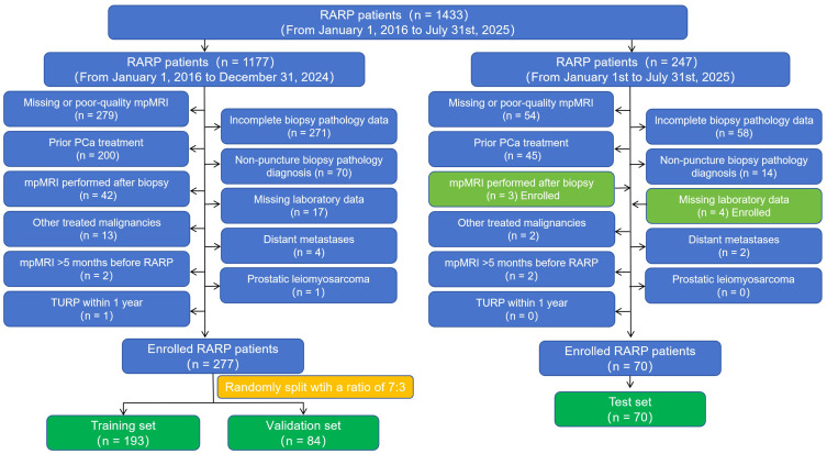 Figure 1
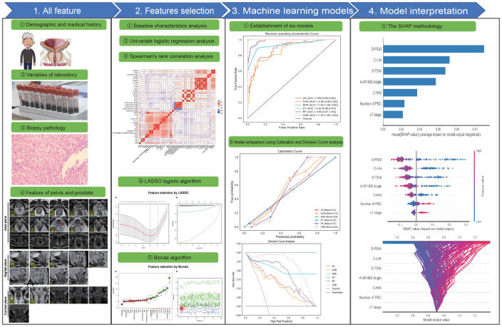 Figure 2
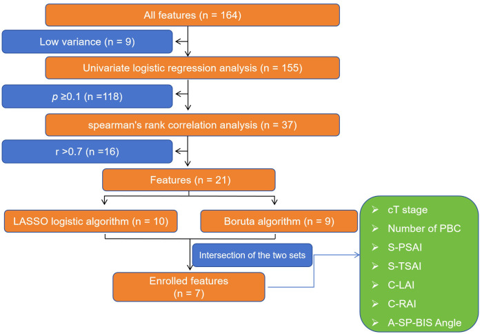 Figure 3
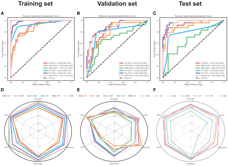 Figure 4
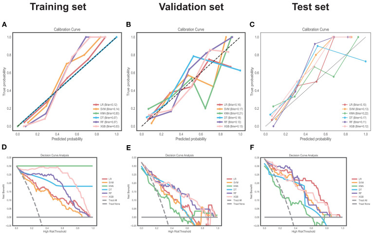 Figure 5
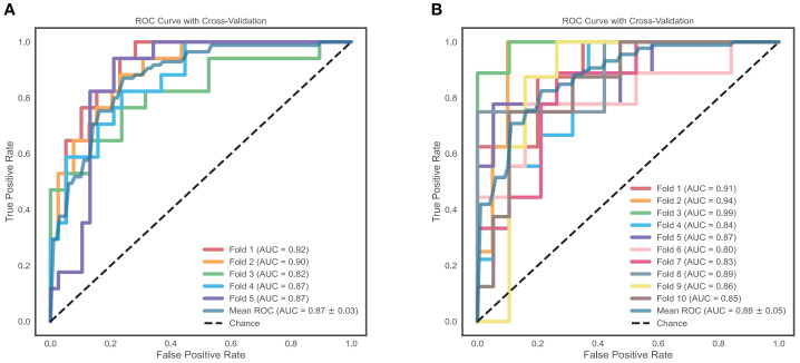 Figure 6
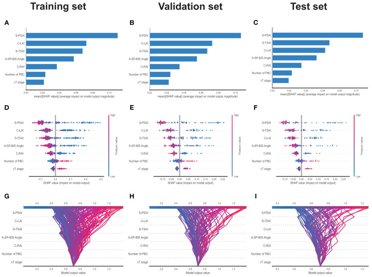 Figure 7
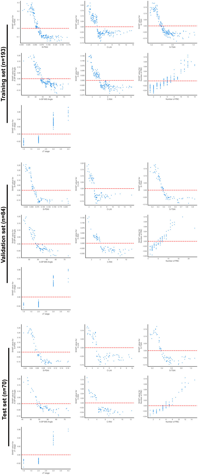 Figure 8
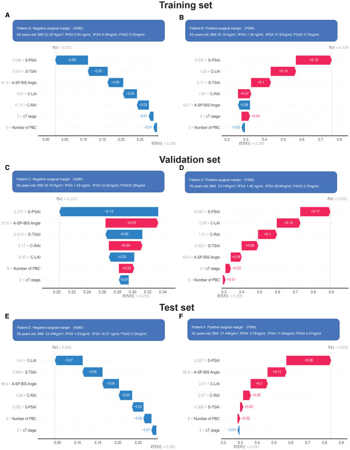 Figure 9
| Characteristics | [ALL] N=277 | [Training set] N=193 | [Validation set] N=84 |
|
|---|---|---|---|---|
| Positive surgical margin (PSM), n(% ) : | 0.837 | |||
| No | 192 (69.3%) | 135 (69.9%) | 57 (67.9%) | |
| Yes | 85 (30.7%) | 58 (30.1%) | 27 (32.1%) | |
| Demographic and medical history data: | ||||
| Age, median (IQR) (year): | 69.0 [65.0;74.0] | 70.0 [65.0;74.0] | 68.5 [64.0;73.0] | 0.32 |
| Body mass index, median (IQR) (kg/m2): | 24.2 [22.4;25.7] | 23.9 [22.0;25.7] | 24.5 [23.0;25.7] | 0.145 |
| Family history of PCa, n(% ) : | 0.303 | |||
| No | 276 (99.6%) | 193 (100%) | 83 (98.8%) | |
| Yes | 1 (0.36%) | 0 (0.00%) | 1 (1.19%) | |
| Abdominal surgery, n(% ) : | 0.634 | |||
| No | 208 (75.1%) | 147 (76.2%) | 61 (72.6%) | |
| Yes | 69 (24.9%) | 46 (23.8%) | 23 (27.4%) | |
| TURP, Over 1 year, n(% ) : | 0.177 | |||
| No | 267 (96.4%) | 188 (97.4%) | 79 (94.0%) | |
| Yes | 10 (3.61%) | 5 (2.59%) | 5 (5.95%) | |
| Smoking, n(% ) : | 0.882 | |||
| No | 168 (60.6%) | 116 (60.1%) | 52 (61.9%) | |
| Yes | 109 (39.4%) | 77 (39.9%) | 32 (38.1%) | |
| Drinking, n(% ) : | 0.801 | |||
| No | 186 (67.1%) | 131 (67.9%) | 55 (65.5%) | |
| Yes | 91 (32.9%) | 62 (32.1%) | 29 (34.5%) | |
| Hypertension, n(% ) : | 1 | |||
| No | 160 (57.8%) | 111 (57.5%) | 49 (58.3%) | |
| Yes | 117 (42.2%) | 82 (42.5%) | 35 (41.7%) | |
| Diabetes, n(% ) : | 0.953 | |||
| No | 222 (80.1%) | 154 (79.8%) | 68 (81.0%) | |
| Yes | 55 (19.9%) | 39 (20.2%) | 16 (19.0%) | |
| Cardiovascular disease, n(% ) : | 0.359 | |||
| No | 234 (84.5%) | 160 (82.9%) | 74 (88.1%) | |
| Yes | 43 (15.5%) | 33 (17.1%) | 10 (11.9%) | |
| Variables of laboratory data, Preoperative: | ||||
| Urinalysis white blood cell, median (IQR) (cell/ul): | 2.00 [1.00;6.00] | 2.00 [1.00;6.00] | 2.00 [1.00;5.00] | 0.972 |
| Platelet, median (IQR) (109/L): | 184 [156;212] | 183 [157;210] | 185 [155;217] | 0.870 |
| Hematocrit, median (IQR) (%): | 42.5 [40.2;44.6] | 42.6 [40.4;44.8] | 42.0 [40.0;44.3] | 0.157 |
| Hemoglobin, median (IQR) (g/L): | 141 [132;148] | 140 [132;149] | 141 [131;147] | 0.519 |
| White blood cell, median (IQR) (109/L): | 5.68 [4.96;6.82] | 5.68 [4.97;6.72] | 5.84 [4.96;6.84] | 0.602 |
| Lymphocyte, median (IQR) (109/L): | 1.61 [1.31;1.97] | 1.60 [1.31;1.90] | 1.65 [1.36;2.03] | 0.461 |
| Monocyte, median (IQR) (109/L): | 0.47 [0.39;0.56] | 0.47 [0.39;0.55] | 0.46 [0.39;0.58] | 0.603 |
| Neutrophil, median (IQR) (109/L): | 3.36 [2.69;4.26] | 3.32 [2.62;4.22] | 3.42 [2.73;4.32] | 0.371 |
| Neutrophil percentage, median (IQR) (%): | 59.1 [53.4;64.1] | 59.1 [53.0;64.0] | 59.2 [54.9;64.9] | 0.517 |
| Neutrophil-to-lymphocyte ratio, median (IQR) : | 2.06 [1.60;2.72] | 2.06 [1.57;2.72] | 2.07 [1.63;2.70] | 0.753 |
| Lymphocyte-to-monocyte ratio, median (IQR) : | 3.50 [2.82;4.32] | 3.52 [2.82;4.24] | 3.48 [2.84;4.60] | 0.905 |
| Platelet-to-lymphocyte ratio, median (IQR) : | 116 [90.1;139] | 118 [90.9;139] | 112 [85.2;138] | 0.592 |
| Monocyte-to-lymphocyte ratio, median (IQR) : | 0.29 [0.23;0.35] | 0.28 [0.24;0.35] | 0.29 [0.22;0.35] | 0.905 |
| SII, median (IQR) : | 372 [269;546] | 370 [267;546] | 377 [271;555] | 0.619 |
| Fasting blood glucose, median (IQR) (mmol/L): | 5.40 [5.00;6.00] | 5.40 [5.00;6.00] | 5.40 [5.00;6.00] | 0.655 |
| Aspartate aminotransferas, median (IQR) (IU/L): | 20.0 [17.0;24.0] | 20.0 [16.0;25.0] | 21.0 [17.0;24.0] | 0.792 |
| Alanine aminotransferase, median (IQR) (IU/L) : | 19.0 [14.0;25.0] | 18.0 [14.0;24.0] | 19.5 [15.0;25.2] | 0.300 |
| DeRitis ratio, median (IQR) : | 1.05 [0.85;1.29] | 1.04 [0.85;1.31] | 1.05 [0.85;1.25] | 0.475 |
| Blood urea nitrogen, median (IQR) (mmol/L) : | 5.90 [4.90;7.00] | 5.90 [5.00;7.00] | 6.05 [4.70;7.12] | 0.975 |
| Serum creatinine, median (IQR) (umol/L): | 81.0 [74.0;94.0] | 81.0 [73.0;93.0] | 83.5 [74.8;96.0] | 0.191 |
| eGFR, median (IQR) (ml/min/1.73m2): | 88.4 [74.4;98.2] | 88.9 [76.9;97.4] | 87.5 [73.0;99.8] | 0.545 |
| Uric acid, median (IQR) (umol/L): | 350 [302;399] | 345 [296;400] | 359 [312;398] | 0.346 |
| Prothrombin time, median (IQR) (s): | 12.9 [12.3;13.5] | 12.9 [12.3;13.4] | 13.1 [12.5;13.6] | 0.279 |
| APTT, median (IQR) (s): | 35.0 [32.4;37.5] | 34.9 [32.5;37.8] | 35.0 [32.4;37.3] | 0.604 |
| Fibrinogen, median (IQR) (g/L): | 2.87 [2.55;3.23] | 2.86 [2.57;3.25] | 2.88 [2.47;3.20] | 0.736 |
| Thrombin time, median (IQR) (s): | 17.6 [17.0;18.4] | 17.7 [17.1;18.4] | 17.4 [16.8;18.5] | 0.122 |
| International normalized ratio, median (IQR): | 0.99 [0.95;1.04] | 0.99 [0.94;1.04] | 1.01 [0.96;1.05] | 0.050 |
| D-dimer, median (IQR) (mg/L): | 0.34 [0.20;0.71] | 0.34 [0.21;0.67] | 0.34 [0.20;0.85] | 0.851 |
| fPSA, median (IQR) (ng/ml): | 1.46 [0.93;2.54] | 1.42 [0.91;2.48] | 1.49 [0.94;2.71] | 0.647 |
| tPSA, median (IQR) (ng/ml): | 13.6 [9.06;25.0] | 13.6 [8.86;26.3] | 13.8 [9.71;22.1] | 0.943 |
| fPSA/tPSA | 0.10 [0.07;0.14] | 0.10 [0.07;0.13] | 0.11 [0.08;0.16] | 0.074 |
| Biopsy pathology: | ||||
| Biopsy Methods, n(% ): | 0.091 | |||
| Conventional | 60 (21.7%) | 47 (24.4%) | 13 (15.5%) | |
| Systematic biopsy | 157 (56.7%) | 110 (57.0%) | 47 (56.0%) | |
| MRI-ultrasound fusion-guided targeted biopsy | 60 (21.7%) | 36 (18.7%) | 24 (28.6%) | |
| Number of biopsy cores, median (IQR): | 12.0 [12.0;12.0] | 12.0 [12.0;12.0] | 12.0 [12.0;12.0] | 0.407 |
| Number of positive biopsy cores, median (IQR): | 5.00 [3.00;7.00] | 5.00 [3.00;7.00] | 5.00 [2.75;7.00] | 0.459 |
| Percentage of PBC, median (IQR) (%): | 41.7 [22.2;58.3] | 41.7 [22.2;58.3] | 41.4 [25.0;60.9] | 0.646 |
| Primary Gleason grade, n(% ): | 0.409 | |||
| 3 | 150 (54.2%) | 102 (52.8%) | 48 (57.1%) | |
| 4 | 118 (42.6%) | 86 (44.6%) | 32 (38.1%) | |
| 5 | 9 (3.25%) | 5 (2.59%) | 4 (4.76%) | |
| Secondary Gleason grade, n(% ): | 0.854 | |||
| 3 | 139 (50.2%) | 99 (51.3%) | 40 (47.6%) | |
| 4 | 113 (40.8%) | 77 (39.9%) | 36 (42.9%) | |
| 5 | 25 (9.03%) | 17 (8.81%) | 8 (9.52%) | |
| Gleason score, n(% ): | 0.749 | |||
| 3+3 | 78 (28.2%) | 55 (28.5%) | 23 (27.4%) | |
| 3+4, 4+3 | 128 (46.2%) | 90 (46.6%) | 38 (45.2%) | |
| 3+5, 4+4, 5+3 | 43 (15.5%) | 30 (15.5%) | 13 (15.5%) | |
| 4+5, 5+4 | 25 (9.03%) | 15 (7.77%) | 10 (11.9%) | |
| 5+5 | 3 (1.08%) | 3 (1.55%) | 0 (0.00%) | |
| Gleason grade group, n(% ): | 0.914 | |||
| 1 | 80 (28.9%) | 55 (28.5%) | 25 (29.8%) | |
| 2 | 68 (24.5%) | 47 (24.4%) | 21 (25.0%) | |
| 3 | 58 (20.9%) | 43 (22.3%) | 15 (17.9%) | |
| 4 | 43 (15.5%) | 30 (15.5%) | 13 (15.5%) | |
| 5 | 28 (10.1%) | 18 (9.33%) | 10 (11.9%) | |
| MRI data: | ||||
| PI-RADS v2, n(% ): | 0.627 | |||
| 2 | 27 (9.75%) | 20 (10.4%) | 7 (8.33%) | |
| 3 | 21 (7.58%) | 14 (7.25%) | 7 (8.33%) | |
| 4 | 54 (19.5%) | 34 (17.6%) | 20 (23.8%) | |
| 5 | 175 (63.2%) | 125 (64.8%) | 50 (59.5%) | |
| Lymph-node invasion: | 0.587 | |||
| No | 273 (98.6%) | 191 (99.0%) | 82 (97.6%) | |
| Yes | 4 (1.44%) | 2 (1.04%) | 2 (2.38%) | |
| Lympho-vascular invasion: | 0.357 | |||
| No | 265 (95.7%) | 183 (94.8%) | 82 (97.6%) | |
| Yes | 12 (4.33%) | 10 (5.18%) | 2 (2.38%) | |
| Perineural invasion: | 0.892 | |||
| No | 258 (93.1%) | 179 (92.7%) | 79 (94.0%) | |
| Yes | 19 (6.86%) | 14 (7.25%) | 5 (5.95%) | |
| Urethral invasion: | 0.398 | |||
| No | 193 (69.7%) | 131 (67.9%) | 62 (73.8%) | |
| Yes | 84 (30.3%) | 62 (32.1%) | 22 (26.2%) | |
| External urethral sphincter invasion: | 0.521 | |||
| No | 265 (95.7%) | 186 (96.4%) | 79 (94.0%) | |
| Yes | 12 (4.33%) | 7 (3.63%) | 5 (5.95%) | |
| Seminal vesicle invasion: | 0.182 | |||
| No | 266 (96.0%) | 183 (94.8%) | 83 (98.8%) | |
| Yes | 11 (3.97%) | 10 (5.18%) | 1 (1.19%) | |
| Rectal invasion: | 1.000 | |||
| No | 276 (99.6%) | 192 (99.5%) | 84 (100%) | |
| Yes | 1 (0.36%) | 1 (0.52%) | 0 (0.00%) | |
| Anterior Fibromuscular Stroma invasion: | 0.291 | |||
| No | 192 (69.3%) | 138 (71.5%) | 54 (64.3%) | |
| Yes | 85 (30.7%) | 55 (28.5%) | 30 (35.7%) | |
| Clinical primary tumor Stage (cT stage), n(%): | 0.963 | |||
| 1 | 27 (9.75%) | 19 (9.84%) | 8 (9.52%) | |
| 2 | 168 (60.6%) | 118 (61.1%) | 50 (59.5%) | |
| 3 | 68 (24.5%) | 47 (24.4%) | 21 (25.0%) | |
| 4 | 14 (5.05%) | 9 (4.66%) | 5 (5.95%) | |
| Axial plane | ||||
| A-TROIM, median (IQR) (mm): | 19.5 [17.5;21.5] | 19.6 [17.4;21.6] | 19.2 [17.5;21.2] | 0.570 |
| A-TLOIM, median (IQR) (mm): | 19.2 [17.2;21.1] | 19.0 [17.2;20.8] | 19.4 [17.3;21.5] | 0.376 |
| A-DOLAM, median (IQR) (mm): | 40.8 [38.3;43.0] | 40.7 [38.6;43.0] | 40.8 [38.1;43.1] | 0.615 |
| A-DILAM, median (IQR) (mm): | 15.2 [14.0;16.6] | 15.2 [13.9;16.6] | 15.2 [14.1;16.7] | 0.894 |
| A-UW, median (IQR) (mm): | 1.28 [1.14;1.41] | 1.27 [1.13;1.41] | 1.31 [1.18;1.45] | 0.361 |
| A-UWT, median (IQR) (mm): | 1.93 [1.72;2.29] | 1.98 [1.76;2.29] | 1.87 [1.63;2.33] | 0.071 |
| A-TMUT, median (IQR) (mm): | 7.69 [6.76;8.63] | 7.65 [6.69;8.67] | 7.77 [6.84;8.56] | 0.895 |
| A-APMUT, median (IQR) (mm): | 7.64 [6.84;8.59] | 7.48 [6.74;8.57] | 7.77 [7.04;8.67] | 0.209 |
| A-RLP, median (IQR) (mm): | 4.93 [3.75;6.62] | 4.86 [3.71;6.50] | 5.12 [4.01;6.74] | 0.247 |
| A-LLP, median (IQR) (mm): | 4.92 [3.78;6.53] | 4.71 [3.68;6.58] | 5.06 [4.01;6.45] | 0.309 |
| A-LLD, median (IQR) (mm): | 18.1 [10.9;27.9] | 18.7 [10.8;27.8] | 16.8 [11.4;28.8] | 0.683 |
| A-CCL-PZ, median (IQR) (mm): | 14.0 [0.00;33.9] | 15.3 [0.00;34.9] | 11.8 [0.00;32.1] | 0.434 |
| A-OID, median (IQR) (mm): | 73.1 [65.4;81.6] | 72.9 [65.4;81.3] | 73.6 [65.7;82.4] | 0.908 |
| A-AAI, median (IQR) (mm): | 9.84 [7.57;13.0] | 9.80 [7.62;12.8] | 9.91 [7.56;13.6] | 0.803 |
| A-ISD, median (IQR) (mm): | 92.0 [88.1;96.2] | 92.1 [88.1;97.5] | 91.2 [88.2;94.8] | 0.317 |
| A-SW, median (IQR) (mm): | 79.4 [68.2;86.3] | 80.0 [68.9;86.0] | 76.3 [66.9;87.2] | 0.212 |
| A-BFW, median (IQR) (mm): | 95.2 [91.1;99.5] | 95.2 [91.2;99.2] | 95.2 [91.0;100] | 0.829 |
| A-ITD, median (IQR) (mm): | 118 [112;125] | 119 [113;125] | 116 [111;123] | 0.154 |
| A-ASP, median (IQR) (°): | 73.3 [68.8;77.5] | 73.7 [69.3;77.5] | 72.4 [68.2;77.9] | 0.285 |
| A-SP-BIS Angle, median (IQR) (°): | 56.4 [52.8;60.1] | 56.9 [52.9;60.6] | 55.8 [52.8;58.6] | 0.183 |
| A-PTD, median (IQR) (mm): | 49.0 [45.6;53.1] | 48.9 [46.0;53.0] | 49.2 [44.6;53.5] | 0.924 |
| A-PAD, median (IQR) (mm): | 49.0 [45.6;53.2] | 48.6 [45.8;53.0] | 49.3 [44.6;53.8] | 0.696 |
| A-LAI, median (IQR) (mm): | 5.24 [3.86;7.61] | 5.18 [3.92;7.45] | 5.54 [3.67;7.74] | 0.903 |
| A-RAI, median (IQR) (mm): | 5.42 [3.63;7.65] | 5.28 [3.47;7.26] | 5.76 [3.87;8.02] | 0.180 |
| A-NTL, n(%): | 0.874 | |||
| 0 | 40 (14.4%) | 27 (14.0%) | 13 (15.5%) | |
| 1 | 179 (64.6%) | 126 (65.3%) | 53 (63.1%) | |
| 2 | 45 (16.2%) | 32 (16.6%) | 13 (15.5%) | |
| ≥3 | 13 (4.69%) | 8 (4.15%) | 5 (5.95%) | |
| A-TLI , n(%): | 0.891 | |||
| No | 40 (14.4%) | 27 (14.0%) | 13 (15.5%) | |
| Yes | 237 (85.6%) | 166 (86.0%) | 71 (84.5%) | |
| Sagittal plane | ||||
| S-PUL, median (IQR) (mm): | 45.0 [41.4;49.6] | 44.2 [41.3;49.3] | 46.0 [41.8;51.2] | 0.151 |
| S-MUL, median (IQR) (mm): | 15.0 [14.0;15.9] | 15.0 [14.0;15.8] | 15.2 [14.1;16.1] | 0.306 |
| S-MUA, median (IQR) (°): | 122 [116;128] | 122 [116;129] | 121 [117;128] | 0.568 |
| S-LASP, median (IQR) (mm): | 40.8 [38.3;43.6] | 40.9 [38.8;43.7] | 39.9 [37.6;43.1] | 0.050 |
| S-API, median (IQR) (mm): | 110 [103;116] | 110 [104;116] | 110 [103;116] | 0.571 |
| S-APM, median (IQR) (mm): | 107 [103;112] | 108 [103;112] | 106 [101;111] | 0.167 |
| S-APO, median (IQR) (mm): | 86.9 [81.4;91.5] | 87.1 [81.7;91.4] | 85.5 [81.0;92.1] | 0.728 |
| S-PD, median (IQR) (mm): | 124 [118;131] | 124 [119;131] | 124 [117;132] | 0.544 |
| S-SD, median (IQR) (mm): | 33.2 [28.6;37.6] | 33.6 [28.3;38.4] | 32.1 [29.0;36.6] | 0.208 |
| S-S1AMCAL, median (IQR) (mm): | 125 [118;133] | 127 [118;133] | 124 [117;132] | 0.453 |
| S-AVPJ, median (IQR) (mm): | 16.0 [12.3;20.4] | 16.8 [12.3;20.9] | 14.9 [12.0;18.5] | 0.033 |
| S-AD, median (IQR) (mm): | 33.4 [30.1;37.3] | 33.4 [30.1;37.6] | 33.4 [29.8;36.9] | 0.688 |
| S-BH, median (IQR) (mm): | 12.4 [6.89;18.1] | 12.1 [6.84;17.6] | 12.7 [7.34;18.9] | 0.345 |
| S-IPPH, median (IQR) (mm): | 0.00 [0.00;5.22] | 1.23 [0.00;5.33] | 0.00 [0.00;5.17] | 0.405 |
| S-UUP, median (IQR) (mm): | 6.55 [2.66;11.1] | 6.35 [2.52;10.4] | 7.12 [2.88;13.3] | 0.107 |
| S-DUP, median (IQR) (mm): | 30.6 [27.5;34.3] | 30.6 [27.6;34.5] | 30.3 [26.7;34.0] | 0.491 |
| S-SA, median (IQR) (°): | 39.1 [35.9;42.4] | 38.6 [35.1;42.3] | 39.3 [37.2;42.9] | 0.180 |
| S-RMA, median (IQR) (°): | 155 [146;163] | 155 [145;163] | 157 [148;163] | 0.343 |
| S-PIA, median (IQR) (°): | 69.1 [66.0;72.7] | 69.1 [66.2;72.8] | 69.0 [66.0;72.4] | 0.631 |
| S-LASP-APO Angle, median (IQR) (°): | 130 [126;135] | 130 [126;135] | 130 [126;134] | 0.967 |
| S-LASP-API Angle, median (IQR) (°): | 101 [95.7;105] | 100 [95.3;105] | 101 [96.3;105] | 0.479 |
| S-LASP-PD Angle, median (IQR) (°): | 59.4 [55.9;62.6] | 59.9 [55.9;63.1] | 58.8 [56.4;61.7] | 0.474 |
| S-APO-API Angle, median (IQR) (°): | 51.2 [45.9;56.5] | 51.2 [45.6;56.5] | 51.3 [47.8;56.3] | 0.581 |
| S-MTSP-IMSPA Angle, median (IQR) (°): | 130 [122;137] | 131 [122;137] | 128 [120;134] | 0.053 |
| S-SP-PA-S1 Angle, median (IQR) (°): | 74.8 [67.8;81.3] | 74.7 [67.5;80.9] | 75.0 [69.7;82.6] | 0.334 |
| S-SP-PA-S5 Angle, median (IQR) (°): | 131 [124;140] | 131 [124;139] | 132 [123;142] | 0.595 |
| S-SP-PA-CA Angle, median (IQR) (°): | 148 [139;159] | 149 [138;158] | 146 [140;160] | 0.914 |
| S-PAD, median (IQR) (mm): | 36.8 [33.0;40.8] | 37.0 [33.0;41.3] | 36.5 [33.2;40.4] | 0.562 |
| S-PCD, median (IQR) (mm): | 45.3 [41.2;51.3] | 45.2 [41.1;50.4] | 45.6 [41.5;52.5] | 0.433 |
| S-AAI, median (IQR) (mm): | 13.2 [10.3;16.4] | 13.5 [10.8;16.6] | 11.8 [9.32;16.1] | 0.084 |
| S-PAI, median (IQR) (mm): | 2.51 [1.89;3.35] | 2.51 [1.94;3.34] | 2.50 [1.80;3.40] | 0.973 |
| Coronal plane | ||||
| C-RST, median (IQR) (mm): | 7.31 [6.15;8.81] | 7.38 [6.12;8.78] | 7.30 [6.20;8.84] | 0.763 |
| C-LST, median (IQR) (mm): | 7.39 [6.14;8.75] | 7.39 [6.11;8.75] | 7.39 [6.16;8.70] | 0.895 |
| C-TRLAM, median (IQR) (mm): | 4.84 [4.03;5.42] | 4.89 [4.06;5.42] | 4.64 [4.00;5.38] | 0.179 |
| C-TLLAM, median (IQR) (mm): | 4.74 [4.16;5.52] | 4.81 [4.21;5.66] | 4.64 [4.08;5.26] | 0.104 |
| C-TVPJ, median (IQR) (mm): | 20.1 [15.3;25.2] | 20.2 [15.5;25.6] | 19.8 [15.1;24.4] | 0.415 |
| C-IPPH, median (IQR) (mm): | 2.79 [0.00;6.24] | 2.79 [0.00;6.49] | 2.87 [0.00;6.07] | 0.733 |
| C-TIP, median (IQR) (mm): | 111 [106;116] | 111 [106;116] | 110 [106;116] | 0.667 |
| C-TTP, median (IQR) (mm): | 104 [100.0;108] | 104 [101;108] | 104 [99.8;106] | 0.429 |
| C-PTD, median (IQR) (mm): | 49.3 [46.0;53.1] | 49.3 [46.2;53.1] | 49.4 [45.8;53.1] | 0.735 |
| C-PCD, median (IQR) (mm): | 41.8 [37.6;47.7] | 41.5 [37.4;47.5] | 42.8 [38.1;48.6] | 0.380 |
| C-LAI, median (IQR) (mm): | 4.32 [2.94;6.10] | 4.22 [2.87;6.10] | 4.36 [3.06;6.09] | 0.495 |
| C-RAI, median (IQR) (mm): | 4.62 [3.17;6.36] | 4.62 [3.06;6.21] | 4.64 [3.26;6.84] | 0.343 |
| Calculated value | ||||
| A-TLAM, median (IQR) (mm): | 12.6 [11.6;13.9] | 12.6 [11.6;14.0] | 12.5 [11.5;13.7] | 0.642 |
| A-PMI, median (IQR) (mm): | 23.1 [17.8;31.2] | 23.1 [17.6;30.9] | 23.1 [17.9;32.2] | 0.814 |
| A-RR, median (IQR): | 0.78 [0.72;0.85] | 0.79 [0.72;0.85] | 0.78 [0.72;0.84] | 0.757 |
| A-TAI, median (IQR) (mm): | 10.7 [7.83;14.4] | 10.6 [7.70;14.1] | 10.8 [8.18;15.3] | 0.366 |
| A-LSAI, median (IQR): | 0.11 [0.07;0.16] | 0.11 [0.07;0.15] | 0.11 [0.07;0.16] | 0.846 |
| A-RSAI, median (IQR): | 0.11 [0.07;0.15] | 0.11 [0.07;0.15] | 0.12 [0.08;0.16] | 0.186 |
| A-TSAI, median (IQR): | 0.22 [0.15;0.31] | 0.22 [0.15;0.30] | 0.24 [0.17;0.32] | 0.358 |
| S-RR, median (IQR): | 0.80 [0.74;0.87] | 0.81 [0.75;0.87] | 0.78 [0.73;0.85] | 0.057 |
| S-TAI, median (IQR) (mm): | 16.0 [12.8;19.3] | 16.3 [13.3;19.3] | 15.0 [11.6;19.2] | 0.167 |
| S-ASAI, median (IQR): | 0.36 [0.27;0.46] | 0.37 [0.28;0.47] | 0.32 [0.25;0.41] | 0.071 |
| S-PSAI, median (IQR): | 0.07 [0.05;0.09] | 0.07 [0.05;0.09] | 0.07 [0.05;0.09] | 0.962 |
| S-TSAI, median (IQR): | 0.43 [0.33;0.53] | 0.44 [0.34;0.53] | 0.39 [0.32;0.49] | 0.115 |
| C-RR, median (IQR): | 0.85 [0.77;0.92] | 0.84 [0.76;0.92] | 0.88 [0.78;0.92] | 0.153 |
| C-TAI, median (IQR) (mm): | 9.19 [6.78;12.2] | 9.15 [6.73;11.7] | 9.25 [6.94;12.8] | 0.440 |
| C-LSAI, median (IQR): | 0.09 [0.06;0.13] | 0.08 [0.06;0.12] | 0.09 [0.06;0.13] | 0.403 |
| C-RSAI, median (IQR): | 0.09 [0.06;0.12] | 0.09 [0.06;0.12] | 0.10 [0.07;0.13] | 0.243 |
| C-TSAI, median (IQR): | 0.18 [0.13;0.25] | 0.18 [0.13;0.24] | 0.19 [0.14;0.26] | 0.319 |
| A-CSAMU, median (IQR) (mm2): | 46.0 [36.6;57.1] | 45.3 [34.8;54.9] | 46.9 [37.6;57.4] | 0.498 |
| MUV, median (IQR) (mm3): | 678 [541;839] | 669 [523;811] | 708 [563;870] | 0.266 |
| PV, median (IQR) (ml): | 44.2 [36.0;57.8] | 44.2 [36.4;57.8] | 44.3 [34.5;58.9] | 0.833 |
| PSAD, median (IQR) (ng/ml/ml): | 0.33 [0.19;0.59] | 0.34 [0.19;0.58] | 0.32 [0.22;0.59] | 0.827 |
| PCI, median (IQR) (mm): | 80.9 [76.6;85.4] | 81.3 [76.4;85.8] | 80.1 [76.6;83.6] | 0.188 |
| PV/PCI, median (IQR), median (IQR) (mm2): | 0.54 [0.44;0.72] | 0.53 [0.44;0.70] | 0.56 [0.42;0.73] | 0.823 |
| S-BH/AD, median (IQR) (mm): | 0.38 [0.21;0.57] | 0.37 [0.21;0.56] | 0.38 [0.21;0.62] | 0.318 |
| BWI, median (IQR): | 2.86 [2.55;3.14] | 2.86 [2.54;3.14] | 2.85 [2.61;3.15] | 0.637 |
| SWI, median (IQR) : | 2.30 [2.01;2.63] | 2.30 [2.02;2.65] | 2.31 [2.00;2.60] | 0.541 |
| PDI , median (IQR) (mm): | 2.77 [2.49;3.08] | 2.74 [2.49;3.08] | 2.81 [2.48;3.07] | 0.878 |
| PDI/PV, median (IQR) (/ml): | 0.06 [0.05;0.08] | 0.06 [0.05;0.08] | 0.06 [0.05;0.08] | 0.947 |
| Robot-assisted radical prostatectomy (RARP) , n(%): | ||||
| TI-MRI-PB, (IQR) (day): | 3.00 [1.00;7.00] | 3.00 [1.00;7.00] | 3.00 [1.75;5.00] | 0.308 |
| TI-PB-S, median (IQR) (day): | 14.0 [10.0;20.0] | 14.0 [10.0;21.0] | 12.5 [8.00;16.0] | 0.056 |
| Inpatient ward, n(% ): | 0.784 | |||
| 1 | 138 (49.8%) | 95 (49.2%) | 43 (51.2%) | |
| 2 | 113 (40.8%) | 81 (42.0%) | 32 (38.1%) | |
| 3 | 26 (9.39%) | 17 (8.81%) | 9 (10.7%) | |
| Surgeons: | 0.208 | |||
| 1 | 89 (32.1%) | 68 (35.2%) | 21 (25.0%) | |
| 2 | 46 (16.6%) | 30 (15.5%) | 16 (19.0%) | |
| 3 | 45 (16.2%) | 34 (17.6%) | 11 (13.1%) | |
| 4 | 40 (14.4%) | 27 (14.0%) | 13 (15.5%) | |
| Others | 57 (20.6%) | 34 (17.6%) | 23 (27.4%) | |
| Concomitant surgical procedures : | 0.165 | |||
| No | 272 (98.2%) | 191 (99.0%) | 81 (96.4%) | |
| Yes | 5 (1.81%) | 2 (1.04%) | 3 (3.57%) | |
| Number of laparoscopic incisions : | 0.835 | |||
| 5 | 128 (46.2%) | 87 (45.1%) | 41 (48.8%) | |
| 6 | 145 (52.3%) | 103 (53.4%) | 42 (50.0%) | |
| Others | 4 (1.44%) | 3 (1.55%) | 1 (1.19%) | |
| Surgical approach: | 0.055 | |||
| Intraperitoneal | 201 (72.6%) | 133 (68.9%) | 68 (81.0%) | |
| Extraperitoneal | 76 (27.4%) | 60 (31.1%) | 16 (19.0%) | |
| Lymph node dissection, n(% ): | 0.12 | |||
| No | 209 (75.5%) | 140 (72.5%) | 69 (82.1%) | |
| Yes | 68 (24.5%) | 53 (27.5%) | 15 (17.9%) | |
| Characteristics | [ALL] N=347 | [Training set] N=193 | [Validation set] N=84 | [Test set] N=70 |
|
|---|---|---|---|---|---|
| Positive surgical margin (PSM), n(% ) : | 0.797 | ||||
| No | 238(68.6%) | 135 (69.9%) | 57 (67.9%) | 46(65.7%) | |
| Yes | 109 (31.4%) | 58 (30.1%) | 27 (32.1%) | 24 (34.3%) | |
| Age, median (IQR) (year): | 70.0 [65.0;74.0] | 70.0 [65.0;74.0] | 68.5 [64.0;73.0] | 71.0 [67.0;76.0] | 0.088 |
| A-SP-BIS Angle (IQR) (°): | 56.6 [53.2;60.2] | 56.9 [52.9;60.6] | 55.8 [52.8;58.6] | 57.0 [54.8;60.7] | 0.102 |
| C-RAI, median (IQR) (mm): | 4.73 [3.24;6.48] | 4.62 [3.06;6.21] | 4.64 [3.26;6.84] | 5.07 [3.82;6.64] | 0.161 |
| C-LAI, median (IQR) (mm): | 4.32 [3.09;6.10] | 4.22 [2.87;6.10] | 4.36 [3.06;6.09] | 4.36 [3.43;6.07] | 0.488 |
| S-PSAI, median (IQR): | 0.07 [0.05;0.09] | 0.07 [0.05;0.09] | 0.07 [0.05;0.09] | 0.07 [0.05;0.09] | 0.907 |
| S-TSAI, median (IQR): | 0.43 [0.33;0.54] | 0.44 [0.34;0.53] | 0.39 [0.32;0.49] | 0.48 [0.35;0.57] | 0.109 |
| cT stage, n(%): | 0.694 | ||||
| 1 | 36 (10.4%) | 19 (9.84%) | 8 (9.52%) | 9 (12.9%) | |
| 2 | 216 (62.2%) | 118 (61.1%) | 50 (59.5%) | 48 (68.6%) | |
| 3 | 79 (22.8%) | 47 (24.4%) | 21 (25.0%) | 11 (15.7%) | |
| 4 | 16 (4.61%) | 9 (4.66%) | 5 (5.95%) | 2 (2.86%) | |
| Number of PBC, median (IQR): | 5.00 [3.00;7.00] | 5.00 [3.00;7.00] | 5.00 [2.75;7.00] | 5.00 [3.00;7.00] | 0.320 |
| Models | Parameter and adjustment range | Optimal parameters |
|---|---|---|
| LR | C': (0.01, 5) | 4.664 |
| penalty': ['l1', 'l2'] | l1' | |
| SVM | C': (0.01, 5), | 4.397 |
| kernel': ['linear', 'rbf'], | 'linear' | |
| gamma': (0.001, 1.0, 'log-uniform') | 0.013 | |
| KNN | n_neighbors': (3, 20) | 9 |
| weights': ['uniform', 'distance'] | distance' | |
| p': (1, 2) | 2 | |
| DT | max_depth': (2, 8), | 4 |
| min_samples_split': (2, 10), | 10 | |
| min_samples_leaf': (1, 5) | 1 | |
| RF | n_estimators': (10, 100), | 76 |
| max_depth': (2, 8), | 8 | |
| min_samples_split': (2, 10), | 10 | |
| min_samples_leaf': (1, 5), | 4 | |
| bootstrap': [True, False], | TRUE | |
| XGB | n_estimators': (10, 100), | 88 |
| max_depth': (2, 8), | 8 | |
| learning_rate': (0.01, 0.5, 'log-uniform'), | 0.047 | |
| subsample': (0.7, 1.0), | 0.828 | |
| colsample_bytree': (0.7, 1.0) | 0.873 |
| Data set | Models | Accuracy | AUC (95% CI) | Sensitivity | Specificity | PPV | NPV | F1 score |
|---|---|---|---|---|---|---|---|---|
| Training set | LR | 0.83 | 0.89 (0.84-0.93) | 0.78 | 0.86 | 0.7 | 0.9 | 0.74 |
| SVM | 0.84 | 0.86 (0.80-0.91) | 0.72 | 0.89 | 0.74 | 0.88 | 0.73 | |
| KNN | 1.00 | 1.00 (1.00-1.00) | 1.00 | 1.00 | 1.00 | 1.00 | 1.00 | |
| DT | 0.89 | 0.93 (0.89-0.97) | 0.88 | 0.90 | 0.78 | 0.95 | 0.83 | |
| RF | 0.94 | 0.99 (0.97-1.00) | 0.91 | 0.96 | 0.9 | 0.96 | 0.91 | |
| XGB | 0.99 | 1.00 (1.00-1.00) | 1.00 | 0.99 | 0.97 | 1.00 | 0.98 | |
| Validation set | LR | 0.75 | 0.84 (0.75-0.92) | 0.89 | 0.68 | 0.57 | 0.93 | 0.70 |
| SVM | 0.70 | 0.80 (0.70-0.89) | 0.96 | 0.58 | 0.52 | 0.97 | 0.68 | |
| KNN | 0.73 | 0.68 (0.56-0.81) | 0.67 | 0.75 | 0.56 | 0.83 | 0.61 | |
| DT | 0.82 | 0.78 (0.66-0.89) | 0.78 | 0.84 | 0.70 | 0.89 | 0.74 | |
| RF | 0.83 | 0.88 (0.80-0.95) | 0.78 | 0.86 | 0.72 | 0.89 | 0.75 | |
| XGB | 0.85 | 0.87 (0.77-0.94) | 0.78 | 0.88 | 0.75 | 0.89 | 0.76 | |
| Test set | LR | 0.91 | 0.94 (0.86-0.99) | 0.83 | 0.96 | 0.91 | 0.92 | 0.87 |
| SVM | 0.89 | 0.90 (0.80-0.97) | 0.79 | 0.93 | 0.86 | 0.90 | 0.83 | |
| KNN | 0.74 | 0.66 (0.51-0.79) | 0.42 | 0.91 | 0.71 | 0.75 | 0.53 | |
| DT | 0.84 | 0.79 (0.65-0.90) | 0.71 | 0.91 | 0.81 | 0.86 | 0.76 | |
| RF | 0.93 | 0.97 (0.94-1.00) | 0.92 | 0.93 | 0.88 | 0.96 | 0.90 | |
| XGB | 0.87 | 0.94 (0.89-0.98) | 0.96 | 0.83 | 0.74 | 0.97 | 0.84 |
| Data set | Models | Z-score |
|
|---|---|---|---|
| Training set | RF vs. LR | 4.6157 | 0.0000 |
| RF vs. SVM | 4.6805 | 0.0000 | |
| RF vs. KNN | -2.4243 | 0.0153 | |
| RF vs. DT | 3.0600 | 0.0022 | |
| RF vs. XGB | -2.4662 | 0.0137 | |
| Validation set | RF vs. LR | 1.3588 | 0.1742 |
| RF vs. SVM | 2.1151 | 0.0344 | |
| RF vs. KNN | 3.7698 | 0.0002 | |
| RF vs. DT | 2.7313 | 0.0063 | |
| RF vs. XGB | 0.9903 | 0.3220 | |
| Test set | RF vs. LR | 1.1390 | 0.2547 |
| RF vs. SVM | 1.9091 | 0.0562 | |
| RF vs. KNN | 4.6554 | 0.0000 | |
| RF vs. DT | 3.1687 | 0.0015 | |
| RF vs. XGB | 1.8528 | 0.0639 |
- —Key Technology Innovation Special of Key Industries of the Chongqing Science and Technology Bureau 10.13039/501100019444
Peer Reviews
No public reviews on file for this paper yet. If you reviewed it on a platform where reviews are public (OpenReview, ICLR, NeurIPS, ICML), you can paste yours below so the community can read it here.
Videos
No videos yet. Explain this paper in a talk, walkthrough, or lecture? Add one.
Taxonomy
TopicsProstate Cancer Diagnosis and Treatment · Radiomics and Machine Learning in Medical Imaging · Colorectal Cancer Screening and Detection
Introduction
Prostate cancer (PCa) is one of the most common malignancies in men worldwide and ranks fifth among cancer-related deaths in males (1, 2). The “Cancer Statistics 2024” report estimates 299,010 new PCa cases and 35,250 related deaths in 2024 (2). Robot-assisted radical prostatectomy (RARP) is the primary surgical treatment for localized PCa and has become the gold standard for radical prostatectomy (RP) (3, 4), significantly improving overall and tumor-specific survival rates (5). By 2013, up to 80% of RPs in the United States were RARP procedures (6).
Positive surgical margin (PSM) in the prostate specimen following RP is a well-established predictor of biochemical recurrence (BCR) (7, 8). The incidence of PSM is influenced by multiple factors, including preoperative prostate-specific antigen (PSA) levels, clinical tumor stage (cT stage), Gleason score/International Society of Urological Pathology (ISUP) grade group, pathological extension of the primary tumor, and others (9–15). Patients with PSM face higher risks of BCR, disease progression, additional treatments, and psychological distress, which negatively impact quality of life (16–18). Given the diversity of RARP patients, preoperative prediction of surgical complexity and prognostic factors is critical for ensuring safety, optimizing scheduling, enhancing care, and reducing costs (19, 20).
Due to the prostate’s deep location within the pelvic cavity, RARP presents challenges such as limited surgical spatial related to prostate size and pelvic anatomy (21, 22). Recent studies have proposed pelvic measurement indicators to characterize pelvic anatomy (21, 23–26) and demonstrated that artificial intelligence (AI) models based on pelvic-prostate spatial features can predict RP surgical difficulty (22, 27–29). However, the stability of AI models depends on the quantity and quality of the training set, and existing models lack integration of radiomics, clinical, and biopsy pathology features, limiting their generalizability.
This study aimed to establish and validate a comprehensive machine learning (ML) algorithm integrating multi-dimensional fusion data (radiomics, prostate/pelvic measurements, clinical, and biopsy pathology features) for preoperative PSM prediction in RARP.
Materials and methods
Study cohorts
This retrospective single-center study was conducted at the Department of Urology, The First Affiliated Hospital of Chongqing Medical University, with collaborative support from co-authors at other institutions for data analysis and imaging feature quantification. This study was approved by the Institutional Review Board (IRB) of our hospital (Approval No. K2023-599) (Supplementary Material 1). As a retrospective study, informed consent from patients was waived. All study protocols were in accordance with the Declaration of Helsinki (30). Clinical data (demographic and laboratory variables), mpMRI data (anatomical features and relevant parameters), and biopsy pathological data were anonymized prior to analysis. PSM was defined as tumor cells at the inked surgical margin, regardless of anatomical location.
Training and validation sets
Patients who underwent RARP between January 2016 and December 2024 were enrolled. Exclusion criteria: (1) Missing or poor-quality mpMRI (n=279); (2) Incomplete biopsy pathology data (n=271); (3) Prior PCa treatment (androgen deprivation therapy, radiotherapy and others; n=200); (4) Non-puncture biopsy pathology diagnosis (such as transurethral resection of the prostate (TURP) and light laser vaporization, which may cause edema of the surrounding tissues) (n=70). (5) mpMRI performed after biopsy (n=42); (6) Missing laboratory data (n=17); (7) Other treated malignancies (n=13); (8) Distant metastases (n=4); (9) mpMRI performed more than 5 months before RARP (n=2); (10) Prostatic leiomyosarcoma (n=1); (11) TURP within 1 year (n=1).
Test set
Patients who underwent RARP between January 2025 and July 2025 were enrolled. Exclusion criteria: (1) Missing or poor-quality mpMRI (n=54); (2) Incomplete biopsy pathology data (n=58); (3) Prior PCa treatment (n=45); (4) Non-puncture biopsy pathology diagnosis (n=14); (5) Other treated malignancies (n=2); (6) Distant metastases (n=2); (7) mpMRI performed more than 5 months before RARP (n=2); (8) prostatic leiomyosarcoma (n=0); (9) TURP within 1 year (n=0). The patient screening flowchart is shown in Figure 1.
Screening flowchart of patients in this study (January 1, 2016, to July 31, 2025). RARP, Robot-Assisted Radical Prostatectomy; mpMRI, Multiparametric Magnetic Resonance Imaging; PCa, Prostate Cancer.
Clinical, mpMRI, and biopsy pathology data collection
Clinical data
A clinician blinded to mpMRI and pathology data extracted 49 features from electronic records, including demographics (age, BMI), lifestyle factors (smoking status, alcohol consumption), comorbidities (hypertension, diabetes), surgical details, laboratory tests (complete blood count, biochemical function, coagulation), and PCa markers (total prostate-specific antigen (tPSA), free prostate-specific antigen (fPSA), fPSA/PSA ratio).
mpMRI data
Imaging was performed using a 3.0 T MR scanner (GE Discovery MR750W, General Healthcare, Milwaukee, USA) with T2-weighted sequences (TR = 3,500 ms, TE = 85 ms, slice thickness=3 mm) and diffusion-weighted imaging (b-values=0, 1,000 s/mm²). Measurements were manually performed by two radiologists (Readers A and B, >8 years of PCa diagnosis experience) using ITK-SNAP (http://www.itksnap.org/). They were blinded to clinicopathological data and assessed Prostate Imaging-Reporting and Data System (PI-RADS) scores, clinical tumour stage, and measured pelvic, prostate, and tumor features. Intraobserver and interobserver correlation coefficients (ICCs) for MRI features ranged from 0.70 to 0.99, indicating good agreement (Supplementary Table 1). Controversial cases were re-evaluated by a senior radiologist (>15 years of experience).
Radiomics features (10 items): PI-RADS score, seminal vesicle invasion (SVI), lymph-node invasion (LNI), lympho-vascular invasion (LVI), perineural invasion, and others.
Anatomical measurements (97 items, Supplementary Table 2, Supplementary Figure 1):
Axial plane (26 items): thickness of right obturator internus muscle (TROIM), thickness of left obturator internus muscle (TLOIM), distance of outer of the levator ani muscle (DOLAM), and others.Sagittal plane (31 items): prostatic urethral length (PUL), membranous urethral length (MUL), membranous urethral angle (MUA), and others.Coronal plane (12 items): right anal sphincter thickness (RST), left anal sphincter thickness (LST), thickness of right levator ani muscle (TRLAM), and others.Calculated values (28 items): thickness of levator ani muscle (TLAM), prostate-muscle index (PMI), roundness ratio (RR), and others.
Biopsy pathology evaluation
All patients underwent transrectal ultrasound-guided prostate biopsy by a single urologist. Biopsy pathology was reviewed by a senior pathologist (>10 years of PCa experience), blinded to MRI and postoperative pathology. Tumor classification was based on the 2016 WHO criteria, with grading via Gleason score and cancer group grades (31, 32). Eight features were recorded, including biopsy method, number of positive biopsy cores (PBC), Percentage of PBC, and others.
Feature extraction and selection
Features with missing rates <10% were included. For imputation, continuous variables were filled with median values, and categorical variables with mode values to ensure comparability.
A four-step selection process was used: (1) Removal of low-variance features (baseline analysis). (2) Initial screening using univariable logistic regression. (3) Remove redundancy using Spearman’s rank correlation analysis (r ≥ 0.7). (4) Select optimal subsets via LASSO and Boruta algorithms, with the final features being the intersection of both.
Hyperparameter tuning
To optimize each algorithm’s performance, we conducted hyperparameter tuning (33). This modeling process utilized a Bayesian hyperparameter search method (34), which systematically evaluated a comprehensive set of hyperparameter values to identify configurations maximizing efficiency and accuracy. Through this detailed and iterative exploration of the hyperparameter space, we were able to fine-tune the models effectively. This meticulous adjustment ensures that our models are precisely calibrated, significantly enhancing their ability to analyze and predict outcomes accurately with the dataset at hand.
ML model construction, validation, and testing
Six ML models for predicting PSM were built: Logistic Regression (LR), Support Vector Machine (SVM), K-nearest Neighbor (KNN), Decision Tree (DT), Random Forest (RF), and Extreme Gradient Boosting (XGBoost). The receiver operating characteristic (ROC) curve analysis, area under the ROC curve (AUC), accuracy (ACC), sensitivity (SEN), specificity (SPE), positive predictive value (PPV), negative predictive value (NPV), and F1 score were calculated to evaluate model performance. To compare the predictive performance and clinical utility of the constructed ML models, the DeLong test, calibration curve analysis with Brier score loss, and decision curve analysis were conducted. A lower Brier score indicated superior model calibration.
Cross-validation of the target model
To further validate model robustness, five-fold and ten-fold cross-validation were performed for the optimal model. In N-fold cross-validation, the dataset is divided into N equal folds; the model is trained on N-1 folds and validated on the remaining fold in each iteration. This process is repeated N times, with the final performance metric derived by averaging results to ensure a robust assessment (35).
Machine learning model interpretation
The optimal model was interpreted using SHAP (Shapley Additive exPlanations) analysis (36, 37). Based on cooperative game theory, SHAP quantifies each feature’s contribution to model predictions by evaluating its marginal impact across all feature combinations, ensuring a balanced representation of feature importance. It provides interpretability at two scales: (1) Local interpretability: clarifies individual predictions by quantifying feature contributions; (2) Global interpretability: synthesizes features’ relative impacts across the entire dataset. The workflow is illustrated in Figure 2.
The overall workflow of this study. LASSO, Least Absolute Shrinkage and Selection Operator; SHAP, Shapley Additive exPlanations; ROC, Receiver Operating Characteristic Curve.
Statistical analysis
SPSS 25.0 (SPSS, Armonk, NY, USA), R software (version 4.3.1; https://www.r-project.org/), and Python (version 3.8.0; https://www.python.org/) were used for statistical analysis. Continuous variables were presented as medians with interquartile ranges (IQRs) and compared using Mann–Whitney U tests. Categorical data were presented as counts (percentages) and compared using chi-square, Fisher’s exact test, or Yates’ continuity correction. Accuracy, sensitivity, specificity, PPV, and NPV based on the optimal cutoff (Youden index) were calculated, with 95% confidence intervals (CIs) estimated using 1,000 bootstraps. A two-tailed P-value < 0.05 was considered statistically significant.
Results
Clinical characteristics
A total of 347 patients (median age: 70 years, IQR: 65.00-74.00 years) were included, with 238 (68.6%) negative surgical margins (NSM) and 109 (31.4%) PSM. No significant differences in clinical, mpMRI, or biopsy pathology features were observed between the training and validation sets (all P > 0.05; Table 1).
Features selection
Based on previous studies (9–15, 21–28) and the authors’ interests. From 164 initial features, 7 key features were retained through four-step screening (Figure 3): (1) 8 low-variance features were excluded (Supplementary Table 3). (2) 119 features unrelated to PSM were excluded via univariable logistic regression analysis (Supplementary Table 4). (3) 16 redundant features (r ≥ 0.7) were removed via Spearman’s rank correlation analysis (Supplementary Figure 2). (4) The LASSO logistic algorithm and the Boruta algorithm retained 10 and 9 features (Supplementary Figure 3), with final features as their intersection. The 7 features (Supplementary Figure 3) included:
▪ Number of positive biopsy cores (Number of PBC).▪ Clinical tumor stage (cT stage).▪ Sagittal plane-posterior spatial anatomical structure index (S-PSAI).▪ Sagittal plane-total spatial anatomical structure index (S-TSAI).▪ Coronal plane-left anatomical structure interval (C-LAI).▪ Coronal plane-right anatomical structure interval (C-RAI).▪ Axial plane-inferior margin of symphysis pubis-bilateral ischial spinous angle (A-SP-BIS Angle).
Screening flowchart of key features for model establishment in this study. cT stage, Clinical primary tumor stage. Number of PBC, Number of positive biopsy cores. S-PSAI, Sagittal plane-Posterior spatial anatomical structure index. S-TSAI, Sagittal plane-Total spatial anatomical structure index. C-LAI, Coronal plane-Left anatomical structure interval. C-RAI, Coronal plane-Right anatomical structure interval. A-SP-BIS Angle, Axial plane-Inferior margin of symphysis pubis - bilateral ischial spinous angle. LASSO, the least absolute shrinkage and selection operator.
No significant differences in these 7 features were observed across the training, validation, and test sets (all P > 0.05; Table 2).
ML model establishment
Table 3 summarizes model parameters, adjustment ranges, and optimal values via Bayesian optimization. Among the six models, KNN and XGB showed high training-set AUCs of 1.00 (95% CI: 1.00-1.00), suggesting overfitting. The RF model achieved optimal balanced performance: (1) Training set: AUC of 0.99 (95% CI: 0.97–1.00), accuracy of 0.94. (2) Validation set: AUC of 0.88 (95% CI: 0.80–0.95), accuracy of 0.83. (3) Test set: AUC of 0.97 (95% CI: 0.94–1.00), accuracy of 0.93. The DT, SVM, and LR models ranked as the second, third, and fourth predicting models in the training set. The DT, LR, and SVM models ranked as the second, third, and fourth predicting models in the validation set. The LR, SVM, and DT models ranked as the second, third, and fourth predicting models in the test set. Model performance metrics are detailed in Table 4 and Figures 4A–F.
Predictive performance of six ML models. This figure presents the Receiver Operating Characteristic (ROC) curve analysis of the established models in the training (A), validation (B), and test (C) sets, as well as the radar plots of the models’ prediction metrics in the training (D), validation (E), and test (F) sets. LR, Logistic Regression; SVM, Support Vector Machine; KNN, K-Nearest Neighbors; DT, Decision Tree; RF, Random Forest; XGB, Extreme Gradient Boosting; AUC, Area Under the ROC Curve; PPV, Positive Predictive Value; NPV, Negative Predictive Value.
Comparison of ML models
DeLong tests confirmed the RF model outperformed LR, SVM, and DT in the training set (all P < 0.05) but not KNN/XGB (overfitting models). In validation and test sets, RF outperformed all five other models (positive Z-scores). In the validation set, RF showed non-significant differences vs. LR/XGB (P > 0.05) but superiority vs. SVM/KNN/DT (P < 0.05). In the test set, RF showed non-significant differences vs. LR/SVM/XGB (P > 0.05) but superiority vs. KNN/DT (P < 0.05) (Table 5).
Also, RF had the lowest Brier scores (except overfitted KNN/XGB models) and well-matched calibration curves (Figures 5A–C), with the highest net benefit in most threshold probabilities at decision curve analysis (Figures 5D–F).
Clinical utility evaluation via calibration and decision curves. Calibration curve analysis of the six models in the training (A), validation (B) and test (C) sets. Decision curve analysis of the six models in the training (D), validation (E) and test (F) sets. "Treat All" and "Treat None" are baselines. Different colors represent models. Brier score, measure of calibration (lower = better).
Robustness checks
Five-fold cross-validation for RF showed fold-specific AUCs of 0.82–0.92, with a mean AUC of 0.87 (95% CI: 0.84–0.90). Ten-fold cross-validation showed fold-specific AUCs of 0.80–0.99, with a mean AUC of 0.88 (95% CI: 0.83–0.93), indicating stable performance (Figure 6).
Five-fold and ten-fold cross-validation of the RF model. (A) Five-fold cross-validation ROC curves of the RF model (AUC values range from 0.82 to 0.92, mean AUC = 0.87, 95% CI: 0.84–0.90); (B) Ten-fold cross-validation ROC curves of the RF model (AUC values range from 0.80 to 0.99, mean AUC = 0.88, 95% CI: 0.83–0.93). The dashed line represents chance (AUC = 0.5). RF, Random Forest; AUC, Area Under the ROC Curve; CI, Confidence Interval.
SHAP interpretation of the RF model
Feature importance rankings were consistent across the training and validation datasets: S-PSAI > C-LAI > S-TSAI > A-SP-BIS Angle > C-RAI > Number of PBC > cT stage (Figures 7A, B). In the test set, the ranking in the test set was: S-SPAI > S-TSAI > C-LAI > A-SP-BIS Angle > C-RAI > Number of PBC > cT stage (Figures 7A-C). Five spatial features (S-PSAI, C-LAI, S-TSAI, A-SP-BIS Angle, C-RAI) were negatively associated with PSM risk, while Number of PBC and cT stage were positively associated (Figures 7D–F). The SHAP decision plot illustrates the influences of all contributing features on the final predicted probability (Figures 7G-I). SHAP dependence plots further clarified feature relationships (Figure 8). Representative cases (NSM vs. PSM) illustrated feature contributions of each of the 7 key features within the RF model (Figure 9).
The SHAP analysis of the RF model. Bar plot of mean SHAP values (feature importance) in the training, validation and test sets (A–C); Bee-swarm plot of SHAP values (color gradients represent feature value by impact) in the training, validation and test sets (D–F); Parallel plot of model output values and feature impact in the training, validation and test sets (G–I); SHAP, Shapley Additive exPlanations; RF, Random Forest; S-PSAI, Sagittal plane-posterior spatial anatomical structure index; C-LAI, Coronal plane-left anatomical structure interval; S-TSAI, Sagittal plane-total spatial anatomical structure index; A-SP-BIS Angle, Axial plane-inferior margin of symphysis pubis-bilateral ischial spinous angle; C-RAI, Coronal plane-right anatomical structure interval; Number of PBC, Number of positive biopsy cores; cT stage, Clinical primary tumor Stage.
SHAP dependence plots for seven features. SHAP dependence plot is a visualization tool in SHAP tools used to analyze the influence of a single feature on model prediction and its interaction with other features, which reveals the direct impact (positive or negative) and nonlinear relationship of features on the prediction results by presenting the relationship between feature values and the corresponding SHAP values.
Representative NSM (A, C, E) and PSM (B, D, F) cases predicted by the RF model. Representative NSM (negative surgical margin) case in the training (A), validation (C) and test (E) sets; Representative PSM (positive surgical margin) case in the training (B), validation (D) and test (F) sets. The distinct contributions of each feature within the RF model for individual predictions are illustrated using the SHAP waterfall plot. RF, random forest. SHAP, SHapley Additive exPlanations.
Discussion
To our knowledge, this is the first study to investigate ML models that integrate clinical, mpMRI, and biopsy pathology data for predicting PSM before RARP. The RF model exhibited excellent performance across the training, validation, and test sets, with its robustness validated via cross-validation. SHAP analysis identified the feature importance rankings, thereby improving model transparency. This innovative approach will improve preoperative surgical risk stratification, optimize clinical decision-making processes, and establish a framework for automated robotic surgery case screening, ultimately advancing the precision and individualization of RARP therapeutic strategies.
Previous studies have identified predictors of PSM, including surgical experience, body mass index (BMI), tPSA, extracapsular extension (ECE), neurovascular bundle (NVB) invasion, cT stage, percentage of positive biopsy cores, number of positive biopsy cores, Gleason score (GS), pathological stage (pT stage), time interval between prostate biopsy and surgery, among others (9–14), but these studies focused on single feature types. Multiparametric MRI (mpMRI), a standard PCa imaging tool (38–41), provides critical anatomical insights, with prior studies linking prostate and pelvic dimensions (e.g., prostate volume (PV), pelvic dimension index (PDI)/PV ratio, prostate-muscle index (PMI), apical depth (AD), symphysis angle (SA), transverse diameter of the pelvic entrance and intertuberous distance (ITD), among others) to PSM risk (21–24, 26, 28, 42, 43). However, focusing exclusively on a single category of features while neglecting their holistic nature when evaluating PSM in RARP offers a limited perspective. This study addressed this limitation by integrating 164 features across multiple domains and screening 7 key predictors through a rigorous multi-step selection process, thereby ensuring the scientific validity and rigor of the selected features.
Optimal hyperparameter tuning is critical for ML performance (44). Data-efficient optimization algorithms, such as Bayesian optimization (44), were employed to automate this process, screening both the parameter adjustment range and optimal parameters. Based on evaluation metrics, KNN and XGB approached or reached a value of 1 for accuracy, AUC, and other metrics, indicating overfitting. The KNN and XGB regression methods were susceptible to overfitting and fit discontinuity, which remain significant challenges in the field (45). In contrast, the RF model obtained suitable AUCs of 0.99 (95% CI: 0.97-1.00), 0.88 (95% CI: 0.80-0.95), and 0.97 (95% CI: 0.94-1.00) in the training, validation, and test sets. The RF outperformed LR, SVM, and DT, indicating superior generalization. Its high accuracy (0.94, 0.83, 0.93), specificity (0.96, 0.86, 0.93), and sensitivity (0.91, 0.78, 0.92) across datasets confirm its predictive reliability. Overall, these results confirm that the RF model is the optimal classifier, consistent with previous studies (46, 47).
Notably, the DeLong test confirmed that in the training set, the AUCs of the RF model were superior to those of LR, SVM, and DT, but lower than those of KNN and XGB. Given that KNN and XGB are overfitting models, these comparisons lack practical significance. The AUCs of the RF model were comparable to those of LR and XGB in the validation set, but superior to those of SVM, KNN, and DT. The AUCs of the RF model were comparable to those of LR, SVM, and XGB in the test set, but superior to those of KNN and DT. The DeLong test confirmed that the overall advantage of the RF model holds, but this advantage has practical value for high-variance models (KNN/DT/SVM models). For LR and XGB models in the validation and test sets, the RF model does not exhibit a significant advantage, which may be attributed to the insufficient sample size of the current validation and test sets. In addition, the RF model exhibited the optimal calibration (lower Brier score, well-aligned calibration curves) and the highest net benefit across most threshold probabilities (decision curve analysis). In conclusion, the RF model demonstrated excellent performance in terms of sensitivity, specificity, accuracy, ROC, and F1 score across the three sets, affirming its predictive reliability and clinical decision-support value. Five-fold and ten-fold cross-validation confirmed the stable performance of the RF model. These results suggest that the RF model could facilitate the identification of surgical difficulty, guide personalized surgical planning, and optimize resource allocation (such as assigning experienced surgeons), thereby reducing the risk of biochemical recurrence after surgery.
ML models are often criticized as “black boxes” (48, 49), which limits their clinical acceptance, particularly in critical applications such as healthcare, where transparency and reliability in clinical decision-making tools are crucial (50, 51). To address this challenge, researchers have focused on developing methods to improve the interpretability of these models, such as SHapley Additive exPlanations (SHAP) analysis, which assigns contribution values to individual features in the dataset to indicate the extent of each feature’s influence on predicted outcomes. This holistic approach enables researchers to identify which features most significantly impact outcomes and whether their influence is positive or negative, thereby promoting the acceptance of ML-based diagnostic or predictive tools in clinical settings (47, 52–56). To our knowledge, this is the first study to investigate ML models based on multi-dimensional fusion data that use SHAP methods for PSM prediction. The contribution relationships of the 7 selected features were successfully visualized using SHAP bar plots, bee-swarm plots, and decision plots. As a result, our study identified that 5 newly discovered spatial features were negatively associated with PSM, with S-PSAI being the most influential. In preoperative PSM prediction, the RF model assigns the highest importance to this feature. Specifically, lower values of S-PSAI, S-TSAI, C-LAI, and C-RAI indicate limited surgical space, which increases surgical difficulty and the risk of tumor residue, prompting surgeons to adjust dissection techniques (such as expanding the resection range or performing more meticulous operations) or assign experienced surgeons. A narrow A-SP-BIS Angle could inform surgical planning (such as adjusting port placement to improve access). However, the number of PBC and cT stage are positively correlated with PSM, consistent with previous studies (11, 12, 15). Surgeons can use feature contributions to prioritize intraoperative vigilance in high-risk regions. SHAP visualizations enhance transparency, thereby improving trust in model-derived decisions and patient understanding and compliance.
This study has several key strengths: (1) Robust data quality: Strict inclusion and exclusion criteria were applied, and enrolled cases underwent rigorous screening; (2) Comprehensive feature integration: Integration of radiomics, prostate and pelvic measurements, clinical, and biopsy pathological features, comprehensively covering factors influencing PSM; (3) Scientific rigor in feature screening: A four-step screening process (low-variance elimination, univariate regression, Spearman correlation-based redundancy removal, and intersection of LASSO and Boruta algorithms) was applied to 164 initial features; (4) Model diversity and validation: Six ML algorithms were used to develop models, and stable predictive models were identified through comparison, with robustness confirmed via sensitivity analysis and N-fold (5-fold and 10-fold) cross-validation; (5) Model interpretability: The SHAP method was employed to clarify the model’s decision-making process, providing valuable insights into its predictive mechanism.
Several limitations of this study should be acknowledged. (1) Retrospective bias: The retrospective design introduced inevitable selection bias, highlighting the need for prospective studies with predefined criteria. (2) Selection bias: The high exclusion rate (primarily due to missing data) may introduce selection bias, as patients with complete data may differ from those excluded. (3) Limited generalizability: Although the dataset is larger than those in previous studies, the single-center Chinese cohort limits global applicability, necessitating external and multi-ethnic validation. (4) Automation limitations: Automatic mpMRI feature recognition is lacking and will be addressed in future work. (5) Restricted surgical scope: Patients undergoing laparoscopic RP were excluded because the surgical assistant’s experience level may impact outcomes, and thus the generalizability of the RF model to RP patients requires further investigation. (6) Data limitations: Genomic data (e.g., PTEN deletion) were not included; future iterations will integrate genomic data and long-term functional outcomes to provide a more comprehensive risk assessment.
In conclusion, ML models based on multi-dimensional fusion data improve PSM prediction in RARP. The RF model, with robust performance and SHAP-based interpretability, enhances preoperative risk stratification, optimizes decision-making, and supports personalized treatment, thereby improving patient treatment compliance and potentially enhancing patient outcomes. Prospective and external validation are required prior to clinical implementation.
The reference list from the paper itself. Each links out to its DOI / PubMed record.
- 1Bray F Laversanne M Sung H Ferlay J Siegel RL Soerjomataram I. Global cancer statistics 2022: GLOBOCAN estimates of incidence and mortality worldwide for 36 cancers in 185 countries. CA Cancer J Clin. (2024) 74:229–63. doi: 10.3322/caac.21834, PMID: 38572751 · doi ↗ · pubmed ↗
- 2Siegel RL Giaquinto AN Jemal A. Cancer statistics, 2024. CA Cancer J Clin. (2024) 74:12–49. doi: 10.3322/caac.21820, PMID: 38230766 · doi ↗ · pubmed ↗
- 3Hu JC Gu X Lipsitz SR Barry MJD'Amico AV Weinberg AC. Comparative effectiveness of minimally invasive vs open radical prostatectomy. Jama. (2009) 302:1557–64. doi: 10.1001/jama.2009.1451, PMID: 19826025 · doi ↗ · pubmed ↗
- 4Patel VR Sivaraman A Coelho RF Chauhan S Palmer KJ Orvieto MA. Pentafecta: a new concept for reporting outcomes of robot-assisted laparoscopic radical prostatectomy. Eur Urol. (2011) 59:702–07. doi: 10.1016/j.eururo.2011.01.032, PMID: 21296482 · doi ↗ · pubmed ↗
- 5Mottet Nvan den Bergh R Briers E Van den Broeck T Cumberbatch MG De Santis M. EAU-EANM-ESTRO-ESUR-SIOG guidelines on prostate cancer-2020 update. Part 1: screening, diagnosis, and local treatment with curative intent. Eur Urol. (2021) 79:243–62. doi: 10.1016/j.eururo.2020.09.042, PMID: 33172724 · doi ↗ · pubmed ↗
- 6Fantus RJ Cohen A Riedinger CB Kuchta K Wang CH Yao K. Facility-level analysis of robot utilization across disciplines in the National Cancer Database. J Robot Surg. (2019) 13:293–99. doi: 10.1007/s 11701-018-0855-9, PMID: 30062641 · doi ↗ · pubmed ↗
- 7Stephenson AJ Kattan MW Eastham JA Dotan ZA Bianco FJJ Lilja H. Defining biochemical recurrence of prostate cancer after radical prostatectomy: a proposal for a standardized definition. J Clin Oncol. (2006) 24:3973–78. doi: 10.1200/JCO.2005.04.0756, PMID: 16921049 · doi ↗ · pubmed ↗
- 8Zhang L Wu B Zha Z Zhao H Jiang Y Yuan J. Positive surgical margin is associated with biochemical recurrence risk following radical prostatectomy: a meta-analysis from high-quality retrospective cohort studies. World J Surg Oncol. (2018) 16:124. doi: 10.1186/s 12957-018-1433-3, PMID: 29970100 PMC 6029044 · doi ↗ · pubmed ↗