DynG: a dynamic scaling factor for thermographic stomatal conductance estimation under changing environmental conditions
Jiayu Zhang, Elias Kaiser, Leo F. M. Marcelis, Silvere Vialet‐Chabrand

TL;DR
Researchers developed a new correction factor called DynG to improve the accuracy of estimating plant stomatal conductance using thermal imaging in changing environmental conditions.
Contribution
The novel DynG correction factor enhances the reliability of stomatal conductance estimation from thermal imaging under fluctuating environments.
Findings
DynG improved the accuracy and stability of stomatal conductance estimates compared to the original method.
DynG estimates matched well with those from lysimetric and gas exchange methods.
DynG successfully distinguished stomatal conductance in different Arabidopsis genotypes.
Abstract
Thermal imaging is a key plant phenotyping and monitoring technique but faces major bottlenecks in accurately and efficiently inferring stomatal conductance (g sw) from leaf temperature. The conductance index (I g) was previously proposed to estimate g sw from thermography by linking temperature differences between real and artificial leaves (ALs) based on the leaf energy balance. However, I g is highly sensitive to environmental fluctuations, hampering interpretation and reducing reproducibility.We developed a simple and novel correction factor (named DynG) for I g that accounts for environmental fluctuations when scaling I g to g sw. This was achieved by capturing temperature variations in a set of ALs with a range of known constant pore conductances. This approach provided the I g–conductance relationship, using ALs as a reference, to infer g sw of real leaves from their measured I…
Genes, proteins, chemicals, diseases, species, mutations and cell lines named across the full text — each resolved to its canonical identifier and authoritative record.
Click any figure to enlarge with its caption.
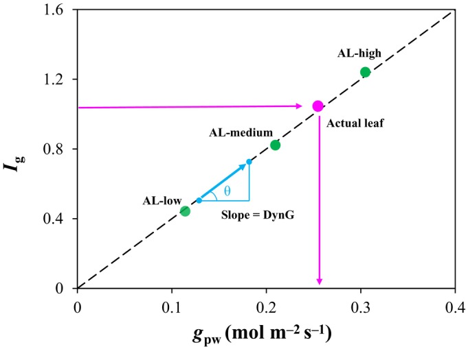 Fig. 1
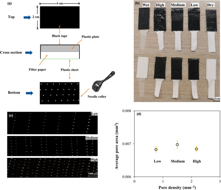 Fig. 2
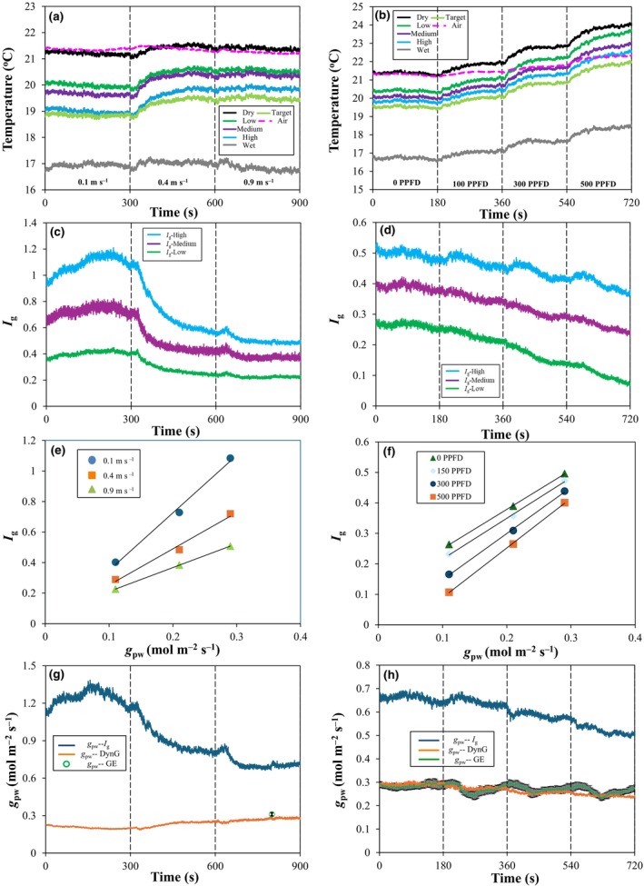 Fig. 3
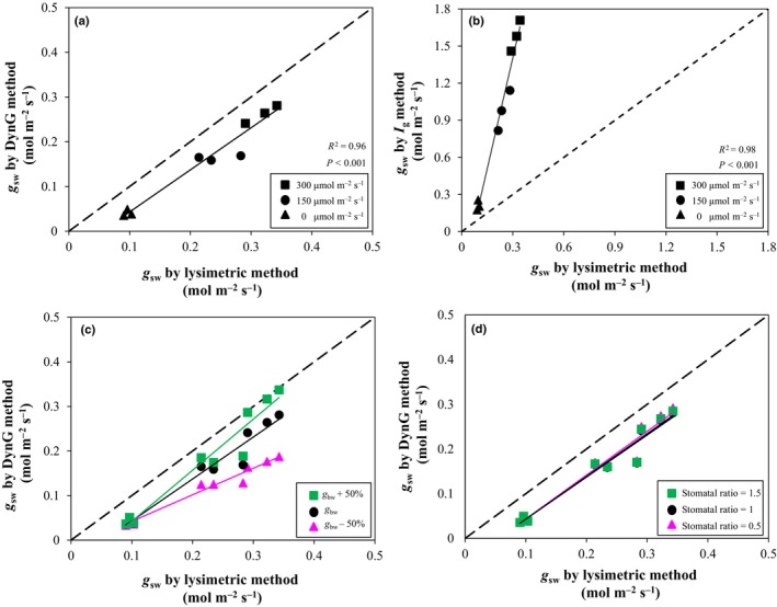 Fig. 4
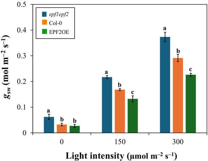 Fig. 5
| Correction factor | Theoretical anatomical maximum |
| ||
|---|---|---|---|---|
|
|
| 1 | ||
|
| 0.09 | 0.06 | 0.08 | 0.10 ± 0.007c |
|
| 0.19 | 0.11 | 0.16 | 0.20 ± 0.006b |
|
| 0.27 | 0.16 | 0.23 | 0.29 ± 0.013a |
| Symbol | Description | Unit |
|---|---|---|
| AL | Artificial leaves | |
|
| Specific heat capacity of humid air | J kg−1 K−1 |
|
| Diffusivity of water vapor in the air | m2 s−1 |
| DynG | Slope of the | dimensionless |
|
| Leaf internal ( | Pa |
|
| Transpiration rate | g m−2 s−1 |
|
| Boundary layer conductance to water vapor | mol m−2 s−1 |
|
| Boundary layer conductance to heat and radiative transfer | mol m−2 s−1 |
|
| Pore conductance to water vapor | mol m−2 s−1 |
|
| Boundary layer conductance to radiative transfer | mol m−2 s−1 |
|
| The sum of cuticular and stomatal conductances to water vapor | mol m−2 s−1 |
|
| Total leaf conductance to water vapor | mol m−2 s−1 |
|
| Slope of the | dimensionless |
|
| Conductance index | dimensionless |
|
| Thickness of plastic film | m |
|
| End correction factor | dimensionless |
|
| Atmospheric pressure | Pa |
| PA | Average pore area | m2 pore−1 |
| PD | Pore density | pores mm−2 |
| PPFD | Photosynthetic photon flux density | μmol m−2 s−1 |
|
| Gas constant | m3 Pa K−1 mol−1 |
| RHair | Air relative humidity | dimensionless |
|
| Net isothermal radiation | W m−2 |
|
| Slope of the curve relating saturation water vapor pressure to | Pa K−1 |
| SR | Ratio of stomatal densities between the ad‐ and abaxial leaf sides | dimensionless |
|
| Air temperature | K |
|
| Temperature of a dry (non‐transpiring) reference | K |
|
| Leaf temperature | K |
|
| Temperature of a wet (fully transpiring) reference | K |
|
| Molar volume of air | m3 mol−1 |
| VPD | Air vapor pressure deficit | Pa |
|
| Leaf absorptance of short‐wave radiation (400–700 nm) | dimensionless |
|
| Long‐wave radiation emissivity of leaf, black electrical tape and filter paper | dimensionless |
|
| Density of air | kg m−3 |
|
| Psychrometric constant | Pa K−1 |
|
| Latent heat of evaporation of water | J kg−1 |
|
| Stefan–Boltzmann constant | W m−2 K−4 |
- —China Scholarship Council10.13039/501100004543
- —Nederlandse Organisatie voor Wetenschappelijk Onderzoek10.13039/501100003246
Peer Reviews
No public reviews on file for this paper yet. If you reviewed it on a platform where reviews are public (OpenReview, ICLR, NeurIPS, ICML), you can paste yours below so the community can read it here.
Videos
No videos yet. Explain this paper in a talk, walkthrough, or lecture? Add one.
Taxonomy
TopicsPlant Water Relations and Carbon Dynamics · Greenhouse Technology and Climate Control · thermodynamics and calorimetric analyses
Introduction
Plants constantly exchange energy and matter with their environment (Lösch, 1994; Jones, 2013). A critical process is the regulation of leaf gas exchange, including water vapor. Stomata are size‐adjustable pores mostly found on leaf surfaces that regulate the balance between carbon assimilation by photosynthesis and water loss through transpiration (E, mol m^−2^ s^−1^). Dynamic regulation of the stomatal aperture is achieved via changes in guard cell turgor pressure, thereby changing stomatal conductance to water vapor (g sw) (Jones, 1998; Yu et al., 2004). g sw is a complex trait influenced by environmental signals (e.g. light intensity and spectrum, air humidity, temperature, and CO_2_ concentration; Casson & Hetherington, 2010; Casson & Gray, 2008), genetics (Pantin et al., 2013; Yu et al., 2015), circadian rhythms (Webb, 2003; Dodd et al., 2004), and acclimation to the growth environment (McElwain et al., 2016; Matthews et al., 2018; Habermann et al., 2019). The considerable inter‐ and intraspecies variation of g sw (Ohsumi et al., 2007; McAusland et al., 2016; Xiong et al., 2018; Faralli et al., 2019) can be measured by phenotyping large populations (Prado et al., 2018) which, combined with genetic mapping technology, can help identify candidate genes. Recently, Pignon et al. (2021) selected genes related to high water use efficiency by monitoring stomatal movement with thermography in a cabinet with stable environmental conditions. However, when scaling up to high‐throughput phenotyping (HTP) platforms in which local microclimate heterogeneity is inevitable, quantifying g sw across large‐scale genotypes under fluctuating conditions becomes a critical challenge. Additionally, g sw is a main determinant of crop yield (McAusland et al., 2023), and continuous monitoring of g sw is critical for fine‐tuning growth conditions and maximizing productivity in controlled‐environment agriculture (Salvatori et al., 2021). However, its practical application remains constrained by the lack of suitable and easy‐to‐use methods, sensors, and models (Kaiser et al., 2024).
The most commonly used method for assessing g sw involves measurements using porometers or infrared gas analyzers that require enclosing the leaf in a chamber. While such measurements are generally accurate, they are lengthy, isolate the leaf from its usual environment, and require relatively expensive equipment (Mayanja et al., 2024). Gravimetric methods (Cirelli et al., 2012) also allow for accurate g sw estimation under controlled environments, as long as boundary layer conductance is known. Other techniques, including microscopy (Sun et al., 2021) and Chl fluorescence (Takaoka et al., 2020), can provide useful measures but are limited in terms of accuracy, throughput, and/or environmental sensitivity. Noncontact thermal imaging is ideal for automatically phenotyping and monitoring g sw of many plants, as variations in leaf or canopy temperature are affected by E, which can be used to estimate g sw (Costa et al., 2013; Driever et al., 2023). Early studies calculated g sw using a full leaf energy balance model that accounted for energy fluxes and mass transfer between the leaf and its microclimate (Jones, 2004). To simplify the application of the leaf energy balance model, Jones (1999b) designed wet and dry reference materials (called ‘references’ hereafter) with similar radiative and aerodynamic properties as real leaves. References can eliminate the need for measuring several environmental parameters (e.g. short‐ and long‐wave radiation) (Leinonen et al., 2006; Guilioni et al., 2008); however, fluctuations in the surrounding environment may compromise their accuracy (Maes & Steppe, 2012). Vialet‐Chabrand & Lawson (2019, 2020) further proposed a thermography‐based method that allows for the continuous monitoring of g sw variations, using any reference material under fluctuating conditions. However, the reliance of the method introduced by Vialet‐Chabrand & Lawson (2019, 2020) on a dynamic leaf energy balance model introduces complexity, limiting its broader adoption. Therefore, a method that is simple, accurate, and robust for estimating g sw under dynamic environments is highly desirable.
The conductance index (I g) is based on temperature differences between actual and reference leaves (Jones, 1999a):
where T dry is the temperature of a dry (nontranspiring) reference, and T wet is the temperature of a wet (fully transpiring) reference, representing the temperatures corresponding to a maximum range of evaporation in a given environment. I g is linearly related to g sw and scaled using the variable G, which is a function of environmental conditions and leaf anatomy (Maes et al., 2016; Pignon et al., 2021; Savvides et al., 2022):
Under a steady environment, G can be considered constant, allowing g sw to be calculated from I g. However, when environmental conditions (e.g. wind speed, air relative humidity, or temperature) change, so do G and I g (Maes & Steppe, 2012; Vialet‐Chabrand & Lawson, 2020), making it impossible to accurately compute g sw. Even in controlled environments, spatial heterogeneity in the microclimate around plants occurs due to uneven air mixing, increasing the difficulty of I g application (Boulard et al., 2004; Poorter et al., 2012). An additional problem is that the I g–g sw relationship is a simplification based on the assumption that both actual and reference leaves evaporate either from both sides simultaneously or from one side only (Guilioni et al., 2008). In other cases (i.e. leaf and references transpiring from different sides), g sw cannot be directly derived from I g, and the uncertain contribution of boundary layer conductance to water vapor (g bw) plays a role in correcting for anatomical differences between actual and reference leaves (Leinonen et al., 2006). While I g offers operational simplicity as an indicator of g sw, its sensitivity to environmental fluctuations and the influence of morphological differences on g bw limit the applicability of I g.
Vialet‐Chabrand & Lawson (2020) proposed using a set of at least three artificial leaves (ALs) with known pore conductance and similar leaf properties, along with ‘wet’ and ‘dry’ references, for deriving G dynamically and converting I g into g sw under any environmental condition. As this idea was never experimentally validated, we explored it further by developing a dynamic scaling factor called DynG and assessing its application under several environmental conditions. The pore conductance of AL was first characterized using microscopy and gas exchange measurements. Then, three Arabidopsis thaliana genotypes differing in stomatal density and size, resulting in large differences in g sw (Franks et al., 2015), were used to test the performance of DynG. Results were validated against a lysimetric method that tracked transpiration‐driven changes in plant weight. Our method solves a critical bottleneck in plant‐ or canopy‐scale g sw phenotyping and monitoring.
Materials and Methods
Theory
Stomatal conductance to water vapor (g sw) can be expressed using leaf temperature (T leaf) and environmental factors based on the leaf energy balance model (Leinonen et al., 2006):
where ρ air is air density (kg m^−3^), C p is the specific heat capacity of air (J kg^−1^ K^−1^), T air is air temperature, s is the slope of the curve relating saturation water vapor pressure to T air, VPD is air vapor pressure deficit (Pa), γ is the psychrometric constant (Pa K ^−1^), R _ ni _ is net isothermal radiation (W m^−2^), g HR is boundary layer conductance to heat and radiative transfer (g HR = 0.92 × g bw + g R), with g R being a radiative conductance (g R = 4×εl×σ×Tair4Cp), σ is the Stefan–Boltzmann constant (W m^−2^ K^−4^), and ε l is leaf long‐wave radiation emissivity (Jones, 2004). Assuming that dry and wet leaves have similar optical and aerodynamic properties to real leaves, they can be used to eliminate R _ ni _ and D, and Eqn 3 can be simplified to:
The value of G that determines the g sw–I g relationship is complex and mainly affected by two conductances: g bw and g HR, suggesting G is sensitive to changes in the environment (wind speed and T air). In addition, G is sensitive to variation in VPD due to the s and γ terms. To address this problem, we used three AL with different pore conductances (g pw) to establish a linear relationship between I g and g pw (Fig. 1) and derive G dynamically. Note that in AL, the conductance to water vapor diffusion is considered constant, unlike in real leaves in which stomatal movement causes g sw to change; therefore, we termed it g pw instead of g sw whenever referring to conductance in AL. The slope between the I g and g pw relationship was named ‘DynG’, which can replace ‘G’ in further equations. I g of actual leaves can theoretically be derived from this relationship under a large range of environmental conditions.
Schematic diagram of DynG. AL‐Low, AL‐Medium, and AL‐High are artificial leaves with different known pore conductance (g pw, mol m−2 s−1). Note that data points are fictitious. The slope θ of the relationship between I g and g pw represents DynG (blue arrows). Pink arrows indicate the projection of the actual leaf data point onto the x‐ and y‐axes.
The linear relationship (Eqn 4) between g sw and I g can only be maintained when the wet AL matches the stomatal ratio (SR; ratio of stomatal densities between the ad‐ and abaxial leaf sides) of an actual leaf (when SR = 0 or 1). This ensures accurate simulation of transpiration patterns and boundary layer characteristics between artificial and actual leaves. In the case of anisolateral leaves (SR = 0–1), there is a difference between g sw and g bw on the upper and lower surfaces, and thus, no explicit expression for g sw can be inferred from I g. By contrast, I g is a linear function of total leaf conductance to water vapor (g tw), which is an integrated expression that combines adaxial and abaxial g sw with g bw (Guilioni et al., 2008). When using an AL wetted on one side, the relationship between g tw and I g is:
SR determines the relative contributions of the upper and lower epidermis in transpiration and g sw (Jalakas et al., 2024) and can be used to derive g sw from g tw, as described in the manual of the Li‐6800 photosynthesis system (Li‐Cor Biosciences, Lincoln, NE, USA; https://www.licor.com/env/support/LI‐6800/manuals.html):
When SR = 1, Eqns 5, 6 can be simplified (Guilioni et al., 2008):
g sw can be calculated if DynG and g bw are known. g bw can be estimated using the leaf energy balance with dry and wet AL (see Eqn 10, for details). In this study, the value of g sw includes both stomatal and cuticular components, as the thermal imaging approach does not allow for their separation. However, the contribution of cuticular conductance is typically negligible compared to that of stomatal conductance (Márquez et al., 2022). Gas exchange methods (LI‐6800) also estimate g sw as the sum of stomatal and cuticular conductance.
Experimental materials
Plant material
Seeds of A. thaliana (L.) Heynh Col‐0 (wild‐type (WT)), epidermal patterning factor (EPF) double mutants (epf1epf2) with increased stomatal density relative to WT as well as the EPF2‐overexpressor (EPF2OE) with reduced stomatal density relative to WT (Hara et al., 2009; Hunt & Gray, 2009) were placed in Petri dishes lined with moist filter paper at 4°C in a dark room for stratification. After 3 to 4 d, seeds were transferred to pots (175 cm^3^, 5 × 5 × 7 cm) filled with a standard sterilized substrate (Lensli, Bleiswijk, the Netherlands), and pots were sealed with black polyethylene plastic films to prevent soil evaporation. Pots were moved to a controlled‐environment climate chamber at a photoperiod of 10 h, T air of 23°C : 20°C (day : night), RH_air_ of 70% ± 2%, and ambient CO_2_ of c. 450 ppm. Plants were grown at an average light intensity of 150 μmol m^−2^ s^−1^ provided by GreenPower LED deep red/blue modules (Signify, Eindhoven, the Netherlands). At 21 to 28 d after germination, plants with uniform growth were used for experiments. Three biological replicates per genotype (n = 3) were used for all measurements.
Construction of AL
Five AL were built to create DynG: one fully dry and one fully wet AL each for I g (Eqn 1) and g bw (Eqn 10) calculation, and three AL with fixed, intermediary g pw based on their porosity for determination of DynG (g pw_low < g pw_medium < g pw_high). All AL were made from Whatman filter paper (No. 1, Cytiva, Marlborough, MA, USA) measuring 2 × 4 cm and with a tail extending c. 4 cm from one side (Fig. 2b). The tail was submerged in a water‐filled test tube (except for the dry AL; Supporting Information Fig. S1) to maintain stable E during the experiment (for at least 1 h; Fig. S2). The filter paper was attached to a polystyrene plastic plate (for support) using double‐sided carpet tape (HEMA, Amsterdam, the Netherlands; Fig. 2a). The top of the plate was covered with black electrical tape, which had an absorptance of 0.96 in the 400‐ to 700‐nm wavelength range and emissivity of long‐wave radiation (ε) of 0.97. In the three intermediate AL, the bottom of the filter paper was covered with a black polyethylene film (a = 0.95, ε = 0.97). A needle roller (URAQT, Shenzhen, China; needle length = 1 mm) was purchased from Amazon and was used to punch holes into the plastic films (Fig. 2a). The needle roller was rolled across the plastic film either once, twice, or three times to create AL with different pore density (and thus different g pw). Dry and wet leaves were left uncovered to ensure zero evaporation by dry leaves and unrestricted evaporation by wet leaves. Note that wet leaves were designed to evaporate only from the bottom surface; this approach prevents potential variations in radiation absorption caused by water films forming on the upper surface, as would be the case with wet leaves wetted on both sides (Brissinger et al., 2014). The edge of the plastic film was wrapped around the polystyrene plate from all sides (except for the end) and thus created a relatively closed space, ensuring minimal evaporation from nonporous areas. Gloves were worn when making AL to prevent grease on the hands from sticking to the surface and affecting evaporation. As filter paper may degrade and change properties, a set of new AL was prepared before each experiment. AL were found to be highly repeatable in their characteristics, as we found close agreement in pore conductance (measured using gas exchange; Li‐6800 photosynthesis system) between three separate replicates (Fig. S3).
Artificial leaves (ALs) with known pore conductance. (a) Schematic of AL including black tape, plastic plate, filter paper, and porous plastic film (thickness = 0.02 mm). (b) Top and bottom sides of five AL. From left to right: wet, high (g pw_high), medium (g pw_medium), low (g pw_low), and dry. Bar, 1 cm. (c) Images of AL with g pw_low (top), g pw_medium (middle), and g pw_high (bottom) under the microscope; bar, 1000 μm. (d) Average pore area (mm2) and density (mm−2) of the three intermediate AL. Data points show mean ± SE (n = 3).
Measurements
Characterization of AL
The porosity of the three intermediate AL was measured with a stereomicroscope (Leica MZ APO MSV269, Leica Microsystems, Wetzlar, Germany), which was connected to a color camera (Axiocam 305 color, Zeiss International, Oberkochen, Germany). The obtained images (Fig. 2c) were processed with imagej (v.1.53, 64‐bit). Average pore area (mm^2^) and density (pores mm^−2^) were calculated based on 8 to 16 pictures (Fig. 2d). From these measurements, the theoretical anatomical maximum g pw (mol m^−2^ s^−1^) of each plastic film was estimated following Dow et al. (2014) (Table 1):
where PD is pore density (pores m^−2^), D is the diffusivity of water in the air (m^2^ s^−1^), PA is the average pore area (m^2^ pore^−1^), V is the molar volume of air (m^3^ mol^−1^), l is the thickness of the plastic film (m), and n is an end correction factor (see Table 2, for symbol description and units). In AL, water vapor forms ‘vapor shells’ at each pore, which accumulate near the pore outlet and may interfere with each other, resulting in longer or more complex vapor diffusion paths, thus adding diffusion resistance (Lehmann & Or, 2015). This phenomenon is known as end correction resistance (R end).
Table 1: Comparison between theoretical maximum g pw based on porosity and measured g pw using gas exchange.
A distance may exist between the pores in the plastic film and the transpiring surface of filter paper, which affects the degree of interaction of the vapor shells and the diffusion path of water vapor. Therefore, correction factors such as one‐end (n = π/4), two‐end (n = π/2), or no correction (n = 1) were considered to quantify the additional diffusive resistance. The one‐end and two‐end correction factors account for vapor shells formed only at the outer ends or both ends of the stomatal cavity, respectively, while no correction represents an intermediate value.
Experimental setup
Measurements were conducted in an enclosure covered with black light‐proof fabric (210 × 120 × 75 cm) to maintain a stable environment, which was located in a temperature‐controlled laboratory with T air of 20°C (Zhang et al., 2024). An infrared thermal camera (FLIR A655sc; FLIR system, Inc., Wilsonville, OR, USA) with an uncooled microbolometer detector (resolution: 640 × 480 pixels; spectral range: 7.5–14.0 μm; noise equivalent temperature difference: <30 mK) was mounted on a tripod and placed on the left side of the enclosure. Temperature changes of real and ALs were continuously captured using the researchir max software (FLIR, v.4.40.12.38). Software settings included the distance between the camera and objects (0.6 m), atmospheric conditions (T air and RH_air_), and reflected temperature (temperature of a crumpled sheet of aluminum foil near the target object, set to ε = 1; (Usamentiaga et al., 2014)). T air and RH_air_ were monitored every 0.1 s by a sensor (SHT‐45; Sensirion, Stafa, Switzerland) connected to a digital reader (SEK‐SensorBridge; Sensirion). An electrical fan was placed next to the thermal camera to ensure air mixing, and wind speed was measured using an anemometer (Voltcraft PL‐135 HAN; Conrad Electronics, Hirschau, Germany). A LED light source (Elixia; Heliospectra AB, Göteborg, Sweden) containing a blue (peak: 450 nm), red (660 nm), and white LED channel, located on the right side of the enclosure, provided illumination. Leaf light absorptance of Arabidopsis genotypes was measured with a spectrophotometer connected to an integrating sphere and was determined to be WT: 0.84 ± 0.004 (mean ± SEM, n = 3), EPF: 0.84 ± 0.003, and epf1epf2: 0.85 ± 0.006, respectively. No significant differences between genotypes were detected (P = 0.68).
Experimental design
Testing the performance of I
g and DynG
Five reference AL and another target AL were placed under three wind speeds (0.1, 0.4, 0.9 m s^−1^; in darkness) and four light intensities (0, 100, 300, 500 μmol m^−2^ s^−1^). The target AL was created by the same procedure as the ‘High’ reference AL (‘Construction of AL’ in the Materials and Methods section); its g pw value remains constant regardless of changes in the surrounding environment, thereby serving as a benchmark to test the performance of I g and DynG on g pw estimation under dynamic conditions. The distance between the fan and AL was modified to ensure that all AL experienced similar wind speeds. A LI‐180 spectrometer (LI‐COR, Lincoln, NE, USA) was used to ensure homogeneous light intensity near AL. Temperature kinetics of AL were recorded, and I g of intermediate AL was calculated using Eqn 1. The target AL was measured using a gas exchange system (Li‐6800). The gas exchange cuvette was set to two different sets of environmental conditions to provide g pw benchmark data in wind speed and light intensity tests: The first set was 300 μmol s^−1^ air flow rate, 21°C T air, 40% RH_air_, and 5‐min darkness for wind speed test (g pw = 0.31 ± 0.012 mol m^−2^ s^−1^). The second set of conditions was 300 μmol s^−1^ air flow rate, 40% RH_air_, and four light intensities (0, 100, 300, 500 μmol m^−2^ s^−1^, each lasting 3 min), and leaf temperatures of 19.5, 20.0, 20.7, and 21.8°C, corresponding to AL temperatures in the thermal imaging setup under the same light intensities. g pw was measured three times by inserting the target AL three separate times.
Distinguishing genotypes with different stomatal density
DynG was tested on the three Arabidopsis genotypes. Studies suggest that SR in Arabidopsis is c. 0.8 to 1 (McAusland et al., 2016; Jalakas et al., 2024; Tulva et al., 2024); so, for simplification, we assumed SR = 1. This assumption satisfies the conditions for using Eqn 7 to obtain g sw. One replicate per genotype and five AL were placed side by side under the LED lamp (Fig. S4a). Since Arabidopsis leaves had a lower light absorptance (0.84) than AL (0.96), plants were placed c. 2 cm closer to the light source than AL, and a LI‐180 spectrometer was used to ensure identical light intensity between AL and plants. Wind speeds (0.4 m s^−1^) around plants and AL were homogenized by adjusting their positions relative to the fan. Objects were then subjected to 0, 150, and 300 μmol m^−2^ s^−1^ for > 1.5 h per photosynthetic photon flux density (PPFD) to ensure stable g sw. Five nonoverlapping leaves per plant were selected for T leaf recordings; target areas on these leaves were outside of the pot's diameter to prevent interference with the temperature of the soil and the film cover above the pot. The average temperature of all selected leaf area was used to represent whole‐rosette temperature, and 25 thermograms were recorded per second (25 Hz). I g of AL was determined using Eqn 1, and g sw of Arabidopsis plants was estimated by inputting the obtained I g into the I g f(g pw) function.
Method validation
Validation of g
pw with gas exchange measurements
Calculated g pw was validated using a gas exchange system (LI‐6800) equipped with a 2‐cm^2^ Chl fluorometer cuvette. Each AL with known g pw was created in triplicate. Before measurements, the tails of AL were immersed in water‐filled tubes for 1 h in the laboratory, at 20°C T air and 40 ± 5% RH_air_. The bottom evaporating surface of the AL was squeezed vigorously using dry tissues to ensure that no droplets adhered to it. Environmental conditions in the gas exchange cuvette were set to 300 μmol s^−1^ air flow rate, 21°C T_air_, 40% RH_air_, and darkness. G pw was measured after 5 min of stabilization (Fig. S3).
Comparison between DynG and lysimetric method
Changes in plant weight due to E were measured to verify DynG. To prevent evaporation from the substrate, pots were wrapped in black plastic film. Col‐0 plants adapted to different light intensities (0, 150, and 300 μmol m^−2^ s^−1^; > 1.5 h per PPFD) were placed on a precision scale (FPRS822; Thermo Fisher Scientific Inc, Leicestershire, UK) in the same setup, which automatically recorded the weights per second, and were subjected to either 0, 150, or 300 μmol m^−2^ s^−1^ for 20 min (Fig. S4b). The thermal camera captured leaf and AL temperature to determine I g. Leaves were removed from the pot, placed on a whiteboard next to a ruler, photographed, and leaf area per plant was estimated using imagej (v.1.53, 64‐bit). E (in g m^−2^ s^−1^) was calculated by estimating the slope of weight loss per unit time, divided by leaf area. g sw was obtained as described previously (see the ‘Comparison between DynG and lysimetric method’ section) and was used to calculate E as modified from Vialet‐Chabrand & Lawson (2020):
where 0.018 is the molecular weight of water (kg mol^−1^), e _ s _ is the leaf internal vapor pressure (Pa) at saturation, and e _ a _ is the air vapor pressure (Pa).
We additionally applied the lysimetric method to calculate g sw using E as input, and compared these g sw values with those obtained through the DynG method, using Col‐0 (n = 3). Furthermore, we compared the g sw calculated by I g (g sw = I g as used in Pignon et al., 2021) with the results of the lysimetric method.
Estimation and validation of g
bw
Based on the steady‐state leaf energy balance, the equation proposed by Vialet‐Chabrand & Lawson (2020) was modified to calculate g bw by using dry and wet leaves:
where ε _ B _ is the emissivity of the upper surface of AL (0.97 for black electrical tape), ε _ F _ is the emissivity of the lower surface of AL (0.95 for filter paper), λ is the latent heat of evaporation of water (J kg^−1^), (0.92 × R × T wet)/P atm is a conversion factor for g bw from heat transfer (m s^−1^) to gas exchange (mol m^−2^ s^−1^), where R is the gas constant (8.3145 J mol^−1^ K^−1^). A sensitivity analysis was performed to characterize the extent to which changes in g bw (± 50%) and SR (0.5 < K < 1.5) in Eqn 7 affect g sw.
To further verify g bw obtained through Eqn 10, a comparison was made with g bw values derived using the lysimetric method. Dry and wet references were placed on the precision scale for 0.5 h in the dark (Fig. S5), and the change in weight was recorded (no change in weight was noticed in the dry reference). As g sw was considered infinite in the wet leaf, Eqn 10 was rewritten as:
This experiment was repeated three times, with new dry and wet ALs being made each time.
Data analysis
Eqns (Eqn 2), (Eqn 3), (Eqn 4), (Eqn 5), (Eqn 6), (Eqn 7), (Eqn 8), (Eqn 9), (Eqn 10), (Eqn 11) were implemented in R (R project, v.4.2.0). For mean testing, the normality of residuals was tested using a Shapiro–Wilk test. A one‐way ANOVA was performed to test for significant differences between Arabidopsis genotypes, and a Tukey's Honestly Significant Difference (HSD) post hoc test was used for mean separation. Statistics were made in R using the aov() and TukeyHSD() functions. A Student's t‐test was used to compare paired samples (dry and wet references) in the g bw validation. All codes are available on GitHub (https://github.com/jiayu0903/dynamic‐conductance‐index.git). A spreadsheet containing an example of calculating g bw (Eqn 10), g sw (Eqn 7) and E (Eqn 9) based on DynG and microclimatic parameters is also provided in Dataset S1.
Results
g
pw of intermediate artificial leaves (ALs)
The g pw of the three intermediate AL that differed in porosity followed the expected trend, namely: g pw_high > g pw_medium > g pw_low (Table 1; P < 0.05). This trend was evident both for calculated values based on measured porosity and from gas exchange measurements on AL. Accounting for the water vapor shell around the pores, we further found that using the one‐end correction factor (n = π/4), values of calculated g pw were very close to measured g pw (Table 1). By contrast, we found that using no (n = 1) or a two‐end correction factor (n = π/2) would underestimate true g pw.
I
g and DynG under dynamic environmental conditions
We tested the performance of DynG by exposing five AL and one target AL to a range of wind speeds and light intensities. Except for the target AL, the temperature kinetics of intermediate AL consistently stayed within the limits set by wet and dry references, with the ‘High’ AL achieving the most and ‘Low’ the least cooling, respectively (Fig. 3a,b). As wind speed increased, the temperature of all AL gradually increased (Fig. 3a; except for the dry and wet reference, which showed a small reduction under high wind speed). The temperature difference between dry and wet references showed a similar trend, increasing with wind speed and light intensity (Fig. S6a,b). Temperatures of air (T air) and of the dry reference were nearly identical under different wind speeds (Fig. 3a), but diverged under different light intensities, as the dry reference heated up with increasing PPFD (Fig. 3b).
DynG accurately captures the pore conductance (g pw) of an artificial leaf (AL) with known porosity, whereas I g does not. (a,b) temperature of AL (dry, low, medium, high, wet, and target) and air (T air). (c,d) I g kinetics of three intermediate AL. (e,f) relationships between I g and g pw of three intermediate AL (Table 1). (g,h) comparison between g pw as inferred using I g (g pw–I g; Eqn 1) or DynG (g pw‐DynG; Eqn 7), or as measured using gas exchange (g pw‐GE; means ± SE, n = 3) on the target AL. The left column shows effects of wind speed (0.1, 0.4, and 0.9 m s−1), while the right column shows effects of PPFD (0, 100, 300, and 500 μmol m−2 s−1). Vertical dotted lines show times at which a change in these factors occurred.
Although g pw of a given AL is constant, I g reduced with increases in either wind speed or PPFD (Fig. 3c,d). Using the three intermediate AL, we found that the slope of the I g vs g pw relationship (DynG) was highly linear and decreased when wind speed and PPFD increased (Fig. 3e,f). The g pw of target AL as inferred from I g (g pw–I g; Eqn 1) showed reductions as wind speed or light intensity increased (Fig. 3g,h). By contrast, g pw as inferred from DynG (g pw‐DynG; Eqn 7) was comparably stable and closely aligned with the value of g pw as measured using gas exchange (g pw‐GE; Fig. 3g,h). We also observed that as PPFD increased, both g pw‐DynG and g pw‐GE showed a slight decrease (Fig. 3h).
DynG validation and sensitivity analysis
Whole‐plant E of Col‐0 plants was determined by either using DynG (Eqn 7) or through the rate of weight loss (Fig. S7). Before estimating E, g bw of the dry and wet reference (Eqn 10) was validated by tracking weight loss of the wet reference, and no significant difference between methods was found (Fig. S5). Whole‐plant E or g sw as determined by either DynG or the lysimetric method showed strong positive linear correlations (R ^2^ = 0.96–0.97), but with a consistent bias toward the lysimetric method. Additionally, values of g sw as calculated using I g strongly deviated from the 1 : 1 line when compared with the lysimetric method (Fig. 4a,b), confirming that DynG can provide much more accurate estimates of g sw than I g.
Validation of DynG by the lysimetric method, and sensitivity analysis of key parameters. Comparison of stomatal conductance to water vapor (g sw) of Arabidopsis Col‐0 by using lysimetric between (a) DynG methods (Eqn 7) and (b) I g methods (Eqn 1) at different PPFD and low wind speed (c. 0.2 m s−1). Sensitivity analysis of g sw by DynG when (c) boundary layer conductance to water vapor (g bw) changed by ±50% and (d) stomatal ratio (SR) changed from 0.5 to 1.5. Note that single‐replicate values are displayed.
To detect the extent to which changes in leaf boundary layer (g bw) and SR affect the estimation of g sw, a sensitivity analysis was conducted. We found that a +50% change in g bw resulted in a 3 to 20% change in simulated g sw, whereas when g bw changed by −50%, the change in g sw was more pronounced, ranging from 7 to 33%, with both effects increasing as light intensity rose (Fig. 4c). On the other hand, different SR (from 0.5 to 1.5) had minimal effects on g sw (Fig. 4d).
Using DynG to distinguish g
sw between genotypes
We tested whether DynG could detect differences in g sw across three Arabidopsis genotypes with varying stomatal density and under different light intensities. All genotypes showed increased g sw when PPFD was increased (Fig. 5). Also, at each PPFD, g sw differed significantly between genotypes (except for Col‐0 and EPF2OE in darkness), and these differences became larger as PPFD increased. This suggested that g sw as derived from DynG can be used to distinguish different genotypes, especially in plants adapted to higher PPFD.
DynG can be used to distinguish stomatal conductance (g sw) between Arabidopsis genotypes at different light intensities. Different letters signify significantly different (P < 0.05) values according to Tukey's HSD test; bars represent the SE of the means (n = 3).
Discussion
A novel method to estimate stomatal conductance
Measuring stomatal conductance (g sw) from thermography has been notoriously difficult, especially in a quickly changing environment. To rapidly and accurately estimate g sw regardless of environmental changes, we propose here a dynamic scaling factor (termed ‘DynG’) using easy‐to‐make leaf replicas. The use of DynG allowed for more accurate predictions of g pw and g sw compared with I g (Figs 3g,h, 4a,b) in dynamic environments, opening new avenues for monitoring stomatal behavior as derived from thermography‐based techniques. Whole‐plant E of WT Arabidopsis (Col‐0) estimated from weight loss correlated very well with E as derived from DynG (Fig. 4a), and further tests demonstrated that DynG successfully distinguished g sw of different Arabidopsis genotypes differing in stomatal density (Fig. 5), suggesting that DynG can be a useful proxy for g sw estimation in HTP.
DynG predicted g
sw accurately under different microclimates
A change in g bw due to variations in wind speed is known to affect I g (Jones, 1999a), which we also observed (Fig. 3c). g bw normally increases with wind speed, and similar results were found in Fig. S6c. It was previously reported that I g was unaffected by incoming radiation (Maes & Steppe, 2012). By contrast, we found that I g decreased when the light intensity increased (Fig. 3d). This difference in results may be attributed to light‐induced microclimate variations affecting the stability of I g. Although g bw was relatively constant, the increased air temperature and reduced air humidity together increased VPD of air, and G is sensitive to VPD. The latent cooling capacity of the AL also increased, amplifying the difference between T dry and T wet (Fig. S6b), and leading to lower I g.
I g of individual AL changed with the ambient microclimate, while DynG is based on the temperature kinetics of dry and wet AL, plus three AL with different and known pore conductance (g pw). These AL can track environmental changes and thus provide I g–f (g pw) at any moment to determine g sw of leaves in the field of view of the thermal camera, representing an improvement compared with I g, which only uses dry and wet leaves (Pignon et al., 2021; Savvides et al., 2022).
Unlike in real leaves in which pore width can change as stomata open or close, any AL should have a relatively fixed g pw with unchanging pore width. Consequently, g pw estimated from different methods should remain stable when the microclimate changes, which was supported by our observations. We found that g pw based on DynG (g pw‐DynG) was relatively stable and close to values determined using gas exchange under a range of PPFD and wind speeds (g pw‐GE). However, this was not the case for g pw based on I g (g pw–I g), which was highly variable (Fig. 3g,h), highlighting the benefit of using DynG under dynamic environments. While DynG demonstrated a robust performance under fluctuating conditions (e.g. wind, light), further testing using mutants that are insensitive to environmental stimuli (e.g. ost1 under different VPD; Merilo et al., 2018) would be informative and valuable for future research.
The g sw calculated from DynG was much closer to values obtained from the lysimetric method than when calculated from I g (Fig. 4b) and showed a more stable trend (Fig. 5b). Arabidopsis leaves normally have stomata on both sides (Pillitteri & Dong, 2013), while AL transpire from only one side, leading to differences in energy balance. The g sw of real leaves is not simply proportional to the I g of AL, and we therefore considered the stomatal distribution and variations in g bw (Guilioni et al., 2008). Interestingly, our sensitivity analysis (Fig. 5d) showed that changes in stomatal ratio (0.5 < K < 1.5) hardly affected calculated g sw, suggesting that for amphistomatous leaves, using K = 1 can simplify the calculations and provide sufficiently accurate results. By contrast, variations in g bw clearly affected calculated g sw (Eqn 7; Fig. 5c), suggesting that accurate estimation of the factors driving g_bw_ is crucial (e.g. wind speed nearby the AL).
The g sw values as estimated through DynG were always slightly lower than those obtained using the lysimetric method (Fig. 5b). This may be due to g bw of AL not fully reflecting that of real leaves. More accurate values of g sw under high‐light intensities can be obtained by increasing g bw by 50% (Fig. 4c). We calculated g bw based on the difference in steady‐state energy balance between a dry and wet AL (Eqn 10), which could be considered an improvement compared with previous methods that required additional energy input, either in the form of heated leaf replicas or through cooling profiles when T leaf was raised above T air (Brenner & Jarvis, 1995; Katsoulas et al., 2006; Stokes et al., 2006; Kimura et al., 2016; Kimura et al., 2020). Although the g bw of AL can be estimated by the dry and wet reference method accurately (Fig. S5), the boundary layer conditions may be different in real leaves compared with AL because of differences in leaf shape, dimensions, presence of trichomes, and edge effects over the lamina (Defraeye et al., 2013; Schymanski & Or, 2016; Kimura et al., 2020). DynG can further quantify the g sw variations of different Arabidopsis genotypes under step changes in light intensity (Fig. 5). The range of g sw obtained from these genotypes was similar to those described in previous studies (Doheny‐Adams et al., 2012; Driever et al., 2023), suggesting that DynG can provide comparable and physiologically meaningful results. Notably, the epf1epf2 double mutant showed significantly higher g sw, consistent with its increased stomatal density (c. 225% higher) and clustering compared with Col‐0 (Hunt & Gray, 2009; Doheny‐Adams et al., 2012), while EPF2OE exhibited reduced g sw, consistent with an c. 80% decrease in stomatal density (Hara et al., 2009; Franks et al., 2015). This agreement with established physiological differences supports the applicability of DynG in resolving genotype‐specific stomatal responses.
Possible applications of DynG
HTP is widely used in plant research and breeding to quantify phenotypic traits across diverse plant species, from model organisms such as Arabidopsis to major crops including wheat, maize, and rice (Yang et al., 2013; Araus & Cairns, 2014; Arend et al., 2016). A bottleneck in HTP related to plant gas exchange is uneven air mixing (Boulard et al., 2004; Katsoulas et al., 2006), such that results at different times or locations on the same platform may be inconsistent, thereby affecting the accuracy and comparability of phenotyping data. Uneven air mixing affects g bw, which in turn affects E and g sw (Monteith, 1995). A typical future application of thermography in HTP could be to place a set of AL in an imaging box on a plant‐to‐sensor platform (i.e. platforms in which plants are moved along fixed phenotyping stations), and utilize DynG for g sw monitoring of each plant entering the box, while providing comparable results that account for the effects of unstable microclimates.
In modern protected cultivation systems such as vertical farms and glasshouses, crop monitoring is essential for improving yields and/or energy use efficiency (van Delden et al., 2021; Steeneken et al., 2023; Kaiser et al., 2024), particularly for key physiological traits such as gas exchange (Kläring & Körner, 2020). Plant–environment interactions are complex, and understanding the plant's real‐time status – which affects its light and water use efficiencies – can significantly aid growers' decision‐making. While experienced growers rely on environmental data to predict plant status, this approach is typically limited to long‐term trends and fails to capture short‐term (e.g. diurnal) or localized changes (Kaiser et al., 2024). This highlights the need for robust and precise sensors to track plant traits over time, and for simple methods to interpret the signals derived from said sensors. Our AL ‐based DynG offers a way to conduct continuous g sw monitoring of crops in their production environment. Furthermore, dry and wet AL may be used for a different kind of sensing: by monitoring temperature changes of AL to calculate g bw in real time and feeding back to the ventilation system, airflow can be intelligently optimized to save electricity (Davies et al., 2008).
Points of attention and limitations
Accurately estimating g pw of AL is a prerequisite for applying DynG. While g pw of a given AL obviously depends on pore size and density, nonlinear diffusion due to the formation of vapor shells may introduce additional diffusion resistance (Lehmann & Or, 2015), which can be corrected by using appropriate ‘end correction’ factors. We found that in our AL, g pw as measured using gas exchange closely matched calculated theoretical maximum anatomical g pw, as long as the latter used an end correction factor of ‘π/4’ (Table 1). This suggests that the AL used by us had a relatively tight structure, effectively reducing the diffusion path of water vapor (Franks & Farquhar, 2001). Additionally, good airflow is necessary, as it affects gas diffusion rate near the surface: Under low wind speed (0.1 ms^−1^), a buildup of humidity (Fig. S6) can result in reduced VPD and impose a temporary reduction on evaporative demand (Grange & Hand, 1987; Fanourakis et al., 2016), thereby affecting g pw.
For plants with a more complex morphology than Arabidopsis, the application of I g and DynG is both limited by heterogeneity in light interception throughout the plant as caused by different leaf angles and orientations (Zhang et al., 2024), as well as the different microenvironments (including air mixing) around the leaves. The use of a set of AL placed at different angles may be a solution for differences in energy balance between such leaves. In addition, absorbed short‐wave radiation accounts for a significant portion of the leaf's energy balance, particularly in the presence of external light input. DynG assumes that real and ALs absorb light equivalently; follow‐up studies could select materials with optical properties similar to those of the target crop to match their leaf absorptance, simplifying the experimental procedure. Additionally, recent research has replicated the microstructure of leaves using soft lithography (Soffe et al., 2019; Bohlim et al., 2021); this could be used to design more realistic AL. In this study, a 'tail' attached to each AL was immersed in water to ensure continuous water supply, allowing the AL to maintain a stable temperature for > 1 h (Fig. S2). To extend the usage time, the AL could be connected to a liquid flow meter or reservoir, as was done in previous studies (Grant et al., 2016; Maes et al., 2016; Schymanski et al., 2017), which can provide a more continuous water supply. However, these designs are more complex and bulkier.
Conclusions
Our novel method provides an easy correction factor ‘DynG’ that can be applied to estimate accurately leaf g sw from thermal imaging with a set of low‐cost leaf replicates under fluctuating environmental conditions. By using DynG to correct the conductance index (I g) and calculate g sw values, we successfully phenotyped different Arabidopsis genotypes without the bias generally observed with I g. This enables the rapid phenotyping or monitoring of g sw and g bw, and provides more comparable and reliable data under different environmental conditions compared with the earlier index, I g.
Competing interests
None declared.
Author contributions
SV‐C, EK and JZ conceived and designed the experiments. JZ performed experiments and analyzed data with the help of SV‐C. JZ, EK, LM and SVC wrote the manuscript. All authors commented and approved the manuscript.
Disclaimer
The New Phytologist Foundation remains neutral with regard to jurisdictional claims in maps and in any institutional affiliations.
Supporting information
Dataset S1 Spreadsheet for calculating g sw based on DynG.
Fig. S1 An overview of the artificial leaves (ALs), including the materials, tools, and perspectives from various angles. Fig. S2 Temperature kinetics of five artificial leaves (wet, dry, high, medium, and low), as well as air temperature (T air), when left in the dark for > 1 h. Fig. S3 Time courses of pore conductance to water vapor (g pw) of three artificial leaves (ALs) in the dark, as determined by gas exchange (Li‐6800). (a) Low g pw, (b) Medium g pw, and (c) High g pw. Each line represents a different replicate. Fig. S4 Overview of experimental setup for distinguishing different genotypes, and DynG validation by the lysimetric method. Fig. S5 Validation of method to determine boundary layer conductance to water vapor (g bw) in AL. Fig. S6 Factors underlying DynG under environmental changes. Fig. S7 Comparison of transpiration rate (E) of Arabidopsis Col‐0 by using lysimetric and DynG methods (Eqn 7) at low wind speed (c. 0.2 m s^−1^).Please note: Wiley is not responsible for the content or functionality of any Supporting Information supplied by the authors. Any queries (other than missing material) should be directed to the New Phytologist Central Office.
The reference list from the paper itself. Each links out to its DOI / PubMed record.
- 1Araus JL , Cairns JE . 2014. Field high‐throughput phenotyping: the new crop breeding frontier. Trends in Plant Science 19: 52–61.24139902 10.1016/j.tplants.2013.09.008 · doi ↗ · pubmed ↗
- 2Arend D , Lange M , Pape JM , Weigelt‐Fischer K , Arana‐Ceballos F , Mücke I , Klukas C , Altmann T , Scholz U , Junker A . 2016. Quantitative monitoring of Arabidopsis thaliana growth and development using high‐throughput plant phenotyping. Scientific Data 3: 1–13.10.1038/sdata.2016.55PMC 498654127529152 · doi ↗ · pubmed ↗
- 3Bohlim N , Lee D , Ryu S , Wilson RA . 2021. Mimicking the surface mechanical properties of rice (Oryzae sativa) leaf using PDMS soft lithography. JMST Advances 3: 1–9.
- 4Boulard T , Fatnassi H , Roy JC , Lagier J , Fargues J , Smits N , Rougier M , Jeannequin B . 2004. Effect of greenhouse ventilation on humidity of inside air and in leaf boundary‐layer. Agricultural and Forest Meteorology 125: 225–239.
- 5Brenner AJ , Jarvis PG . 1995. A heated leaf replica technique for determination of leaf boundary layer conductance in the field. Agricultural and Forest Meteorology 72: 261–275.
- 6Brissinger D , Parent G , Boulet P . 2014. Experimental study on radiation attenuation by a water film. Journal of Quantitative Spectroscopy and Radiative Transfer 145: 160–168.
- 7Casson S , Gray JE . 2008. Influence of environmental factors on stomatal development. New Phytologist 178: 9–23.18266617 10.1111/j.1469-8137.2007.02351.x · doi ↗ · pubmed ↗
- 8Casson SA , Hetherington AM . 2010. Environmental regulation of stomatal development. Current Opinion in Plant Biology 13: 90–95.19781980 10.1016/j.pbi.2009.08.005 · doi ↗ · pubmed ↗