Quantile index predictors using R package hyper.gam
Tingting Zhan, Misung Yi, Inna Chervoneva

TL;DR
The paper introduces an R package called hyper.gam for analyzing single-cell protein expression data to derive functional biomarkers.
Contribution
The novel contribution is a supervised learning framework using quantile functions for biomarker discovery in single-cell data.
Findings
The hyper.gam package converts single-cell data into quantile functions for biomarker estimation.
The package provides tools for estimating integrand surfaces and exploring them visually.
It is designed for heterogeneous protein expression analysis but is applicable to other single-cell data types.
Abstract
Evaluation of single-cell protein expression from immunohistochemistry images is used increasingly in biomedical research. Many proteins are used solely for phenotyping cells in the tumor microenvironment. Other proteins with meaningfully quantitative expression levels provide so-called functional protein biomarkers. There is still a limited number of methods and software tools available for utilizing the entire distributions of single-cell expression levels. We present the R package hyper.gam, providing a supervised learning framework for deriving biomarkers based on single-cell distribution quantiles. The single-cell data are first converted into sample quantile functions, which are then used as predictors in scalar-on-function regression models to estimate the integrand surface. The estimated integrand surface defines the quantile index predictors based on the single-cell expression…
Genes, proteins, chemicals, diseases, species, mutations and cell lines named across the full text — each resolved to its canonical identifier and authoritative record.
Click any figure to enlarge with its caption.
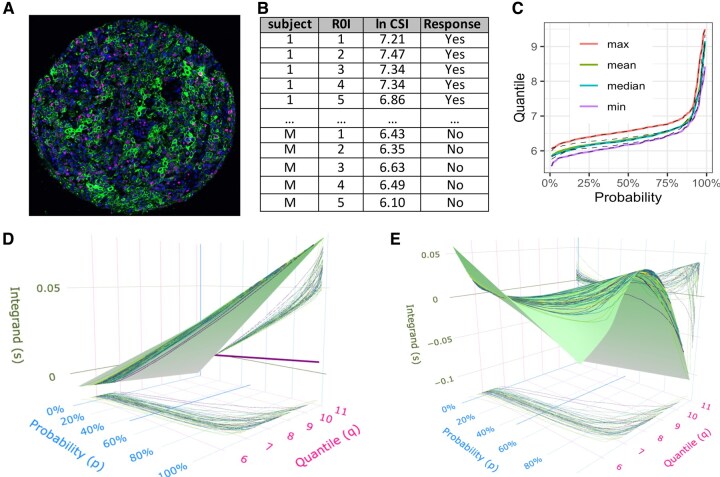 Figure 1
Peer Reviews
No public reviews on file for this paper yet. If you reviewed it on a platform where reviews are public (OpenReview, ICLR, NeurIPS, ICML), you can paste yours below so the community can read it here.
Videos
No videos yet. Explain this paper in a talk, walkthrough, or lecture? Add one.
Taxonomy
TopicsSingle-cell and spatial transcriptomics · Radiomics and Machine Learning in Medical Imaging · Cancer Genomics and Diagnostics
Introduction
Novel biomarkers are increasingly important for optimizing individualized cancer treatment strategy. Multiplex immuno-fluorescence immunohistochemistry (mIF-IHC) and advanced image analysis platforms enable measurement of protein expression in each single tumor cell, but some kind of average expression is usually considered as a potential biomarker. Meanwhile, intra-tumoral heterogeneity of protein expression in cancer cells is well-documented (e.g.Malinowsky et al. 2012, Qian et al. 2017) and may provide additional prognostic value (Supernat et al. 2014, Jacquemin et al. 2022).
Single-cell mIF-IHC data usually include coordinates of the cell centroids and cell signal intensity (CSI) of the protein expression and may be analyzed using spatial statistics approaches (e.g.Yuan, 2016, Wilson et al. 2021). Spatial analysis is especially informative for quantifying interaction between cancer and immune cells in the tumor immune microenvironment (e.g.Creed et al. 2021, Vu et al. 2022, Patrick et al. 2023). A spatial distribution may not be as relevant for quantification of heterogeneity for proteins that serve as functional biomarkers (Wrobel et al. 2023) with quantitative expression levels. The spatial approaches are computationally intense and often have complicated interpretations. Also, virtually all spatial metrics are based on the assumption of stationarity, which means that spatial localization patterns are similar in different regions of the tumor tissue. This assumption is generally not appropriate for the whole tumor tissues that always exhibit spatial heterogeneity of the protein expression of interest (e.g. Masotti et al. 2023).
Recently proposed approach for the distributional analysis of single-cell mIF-IHC data (Yi et al. 2023a) allows capturing intra-tumoral heterogeneity of protein expression by representing the entire distribution of CSIs in a tissue by the empirical/sample quantile function. The quantile function is the inverse of the cumulative distribution function. It is defined on the interval [0, 1] which facilitates the application of the functional data analysis methods. It is well-known that in case of independence between CSI levels and spatial localization of the cells, it is sufficient to consider marginal distribution of CSI without loss of information (e.g. Baddeley, 2013). Even if independence is not the case, considering CSI distributions without spatial localization of the cells may provide similar prognostic value. For example, Ki-67 expression was considered as a marker based on the spatial marked point pattern in Chervoneva et al. (2021) and based on quantiles of marginal CSIs distribution in Yi et al. (2023b), and results for predicting progression-free survival in breast cancer were very similar with and without considering spatial distribution of Ki-67 CSIs. Additional consideration is the much higher computational efficiency of non-spatial analysis approaches, which becomes more important for large volumes of single-cell mIF-IHC data.
In this article, we describe how to derive the Quantile Index (QI) predictors (Yi et al. 2023a, 2025) using the R package hyper.gam. The QI predictors are based on the empirical quantile functions of CSIs distributions in each biological sample. Prior to analysis, the R package groupedHyperframe is used to convert the CSI data into an R object of the groupedHyperframe class. In the first step of analysis, the single-cell data are converted into the sample quantiles of CSIs distributions on a pre-specified grid of probabilities. The sample quantile functions may have to be aggregated if more than two levels of clustering are present in the CSI data. In the second step, a suitable scalar-on-function model (Reiss et al. 2017) is fitted to a training data set with aggregated sample quantile functions as a predictor and a scalar outcome of interest. In the third step, the estimated integrand surface of the scalar-on-function regression model is used to compute a scalar quantile index based on the sample quantile function for each subject in the test dataset. The resulting quantile index can be evaluated as a predictor of outcome of the interest in the test data.
Functionality and analysis
Data structure and processing
Single-cell mIF-IHC imaging data are the result of digital processing of the microscopic images of tissue stained with selected antibodies. Figure 1A shows an example of an mIF-IHC image of a tissue core stained for Ki-67 protein as well as DAPI and cytokeratin. Quantitative pathology platforms, such as Akoya or QuPath, support cell segmentation of mIF-IHC images and quantification of the mean protein expression in each cell. The cell centroid coordinates and cell signal intensities (CSIs) for each stained protein are usually extracted as individual comma-separated values (.csv) files. It is expected that for each independent cluster (subject), a large number of observations are available, capturing information about each cell in the subject tissue. In some but not all cases, single-cell data would come from Regions of Interest (ROI) selected in the whole tissue image. Thus, the ROIs are clustered within subjects, and each ROI includes a large number of single-cell observations. Alternatively, a Tissue Microarray (TMA) may be analyzed with multiple tissue cores per subject. In either case, ROIs or TMA tissue cores represent the lowest level of clustering in the data with a substantially varying number of cells per cluster. Figure 1B illustrates the structure of the mIF-IHC CSI data with two levels of clustering and an outcome of interest (Response). The actual mIF-IHC data sets may include CSI levels for multiple proteins and possibly variables capturing phenotypes of each cell (e.g. cancer, T-cell, macrophage, etc.).
(A) Example of an mIF-IHC image of a tissue core stained for Ki-67 protein (pink) as well as DAPI (blue) and cytokeratin (green); (B) Clustered structure of the mIF-IHC CSI data used for deriving quantile biomarkers; (C) Example of ROI-specific quantile functions for one tissue (dashed black lines) and tissue-specific functions (colored solid lines) aggregated using point-wise max, mean, median, and min of ROI-specific values; (D) Estimated integrand surface for linear QIs based on Ki-67 CSI expression levels with estimated coefficient function β(p) (in purple) shown in the qs-plane; (E) Estimated integrand surface for nlQIs based on Ki-67 CSI expression levels. The contour lines on the integrand surfaces show the paths of integration for computing Ki-67 QIs for a subsample of tissue cores. Projections of these paths onto (p,q) plane show the corresponding Ki-67 CSI sample quantiles. The areas under the projections of the integrand paths onto (p,s) plane are equal to linear QI (D) or nlQIs (E).
Prior to analysis, function as.groupedHyperframe() in the R packages groupedHyperframe is used to convert the CSI data into an R object of groupedHyperframe class. Data example Ki67 in package groupedHyperframe is a grouped hyper data frame, an extension of the hyper data frame defined in package spatstat.geom (Baddeley and Turner, 2005, Baddeley et al. 2015). The numeric-hypercolumn logKi67, whose elements are numeric vectors of different lengths, contains the log-transformed Ki-67 protein expression CSIs in each ∼patientID/tissueID, a nested grouping structure following the nomenclature of package nlme (Pinheiro et al. 2025). The data example Ki67 also contains the metadata, e.g. progression-free survival (PFS), Her2, HR, etc.
Quantile index (QI) biomarkers
Linear quantile index (QI, Yi et al. 2023a) is a predictor in a functional generalized linear model (James, 2002) for outcomes from the exponential family of distributions, or a linear functional Cox model (Gellar et al. 2015) for survival outcomes,
where is the sample quantiles for the i-th patient and is an unknown coefficient function.
Non-linear quantile index (nlQI, Yi et al. 2025) is a predictor in a functional generalized additive model (McLean et al. 2014) for outcomes from the exponential family of distributions or an additive functional Cox model (Cui et al. 2021) for survival outcomes.
where is an unknown bivariate twice differentiable function, which allows the association between the nonlinear quantile index and the functional predictor to vary nonlinearly in both the functional domain p and the value of the functional predictor .
Pipeline for deriving QI biomarkers
Complete R code for the analysis outlined in the following steps can be found in the vignette of package hyper.gam at https://CRAN.R-project.org/package=hyper.gam/vignettes/applications.html, in the section Quantile Index. The vignette covers all technical details, including the R version and key dependencies, in the section Introduction.
Step 1: Compute aggregated quantiles
Function aggregate_quantile() converts each element of the hypercolumn in the groupedHyperframe object into sample quantiles at a pre-specified grid of probabilities . If only one level of clustering is present in the data (e.g. only one ROI or tissue core per patient), the cluster-specific sample quantile function is used as the functional predictor for each patient. In case of multiple lowest-level clusters per patient (e.g. multiple tissueID’s per patientID), the function aggregate_quantile() aggregates the lowest-level cluster-specific sample quantiles into patient-specific functions using point-wise mean, median, minimum and maximum (Fig. 1C). The aggregation must be performed at the level of biologically independent clusters, e.g. ∼patientID, to produce independent aggregated quantile predictors.
Figure 1D and E shows the (aggregated) patient-specific sample quantiles in the horizontal pq-plane with coordinates p (probability) and q (quantile).
Step 2: Estimate integrand surface
Function hyper_gam() estimates a scalar-on-function model with patient-specific aggregated sample quantile functions as a functional predictor. It returns an object of class hyper_gam, which inherits from the gam class of package mgcv (Wood, 2017).
The estimated integrand surface,
is defined for , .
We also implement an optional sign adjustment to ensure a positive correlation of quantile indices with at a user-specified (default ), in order to facilitate the interpretation of quantile indices. The sign-adjusted integrand surface is , where or .
Step 3: Compute quantile index predictor
Function predict.hyper_gam() computes QI and nlQI predictors for a training or independent test data set, based on the estimated integrand surface (3). The resulting QIs or nlQIs can be evaluated as a predictor of outcome of interest in the test data. The QI and nlQI computed in the training data set are expected to be optimistically biased as predictors of outcome because they are optimized on the same data set.
Visualization of integrand surface
Function integrandSurface() creates an interactive htmlwidgets (Vaidyanathan et al. 2023) visualization of the estimated integrand surfaces for the linear (1) or nonlinear quantile index (2) using package plotly (Sievert, 2020).
Snapshots in Fig. 1D and 1E show the estimated integrand surfaces for linear and nonlinear quantile index, respectively, in the training data set. The estimated integrand paths per patient are shown on the integrand surfaces (3), as well as projected to the -plane. In addition, the estimated functional coefficient is shown projected to -plane as a solid line in Fig. 1D.
Discussion
R packages groupedHyperframe and hyper.gam implement a supervised learning framework for deriving single-index biomarkers based on distribution quantiles. The framework was designed to enable derivation of functional protein biomarkers based on single-cell protein expression levels with optimal predictive value for an outcome of interest. In our examples, empirical quantile functions represent CSI levels in mIF-IHC data, but the same methods and implementation are also applicable to any single-cell data from genomics, transcriptomics, proteomics, or metabolomics studies with quantitative expression levels. Currently publicly available single-cell data do not include numbers of subjects sufficient for the proposed supervised learning and testing in an independent data set, but rapidly evolving technologies are expected to produce such large sample data in the nearest future. Thus, the proposed methodology has the potential to facilitate the development of various single-cell omics biomarkers critically needed for personalized medicine.
The reference list from the paper itself. Each links out to its DOI / PubMed record.
- 1Baddeley A. Stochastic Geometry, Spatial Statistics and Random Fields: Asymptotic Methods, Chapter Spatial Point Patterns: Models and Statistics. Berlin, Heidelberg: Springer Berlin Heidelberg, 2013, 49–114.
- 2Baddeley A , Rubak E, Turner R. Spatial Point Patterns: Methodology and Applications with R. London: Chapman and Hall/CRC Press, 2015.
- 3Baddeley A , Turner R. Spatstat: an R package for analyzing spatial point patterns. J Stat Soft 2005;12:1–42.
- 4Chervoneva I , Peck AR, Yi M et al Quantification of spatial tumor heterogeneity in immunohistochemistry staining images. Bioinformatics 2021;37:1452–60.33275142 10.1093/bioinformatics/btaa 965PMC 8208754 · doi ↗ · pubmed ↗
- 5Creed JH , Wilson CM, Soupir AC et al spatial TIME and i TIME: r package and shiny application for visualization and analysis of immunofluorescence data. Bioinformatics 2021;37:4584–6.34734969 10.1093/bioinformatics/btab 757PMC 8652029 · doi ↗ · pubmed ↗
- 6Cui E , Crainiceanu CM, Leroux A. Additive functional cox model. J Comput Graph Stat 2021;30:780–93.34898969 10.1080/10618600.2020.1853550 PMC 8664082 · doi ↗ · pubmed ↗
- 7Gellar JE , Colantuoni E, Needham DM et al Cox regression models with functional covariates for survival data. Stat Modelling 2015;15:256–78.26441487 10.1177/1471082 X 14565526 PMC 4591554 · doi ↗ · pubmed ↗
- 8Jacquemin V , Antoine M, Dom G et al Dynamic cancer cell heterogeneity: Diagnostic and therapeutic implications. Cancers 2022;14:280. 10.3390/cancers 1402028035053446 PMC 8773841 · doi ↗ · pubmed ↗