A range of voltage-clamp protocol designs for rapid capture of hERG kinetics
Chon Lok Lei, Dominic J Whittaker, Monique J Windley, Matthew D Perry, Adam P Hill, Gary R Mirams, Lucia Romero Perez, Arpad Mike

TL;DR
This paper introduces short voltage-clamp protocols to efficiently study the hERG ion channel's behavior, aiding in modeling its function.
Contribution
A novel set of voltage-clamp protocols is proposed for rapid and efficient characterization of hERG channel kinetics.
Findings
The protocols use simple steps and ramps to capture detailed hERG gating data.
They are designed for compatibility with automated patch clamp systems.
The approach can be generalized to study other ion channels.
Abstract
We provide details of a series of short voltage-clamp protocols designed for gathering a large amount of information on hERG (K v11.1) ion channel gating. The protocols have a limited number of steps and consist only of steps and ramps, making them easy to implement on any patch clamp setup, including automated platforms. The primary objective is to assist with parameterisation, selection and refinement of mathematical models of hERG gating. We detail a series of manual and automated model-driven designs, together with an explanation of their rationale and design criteria. Although the protocols are intended to study hERG1a currents, the approaches could be easily extended and generalised to other ion channel currents. Ion channels are proteins that span the membranes of biological cells, and they allow certain ions to flow through them, to cross the membrane (e.g. K +, Na + or Ca 2+).…
Genes, proteins, chemicals, diseases, species, mutations and cell lines named across the full text — each resolved to its canonical identifier and authoritative record.
Click any figure to enlarge with its caption.
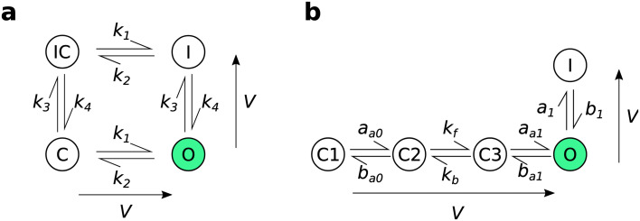 Figure 1
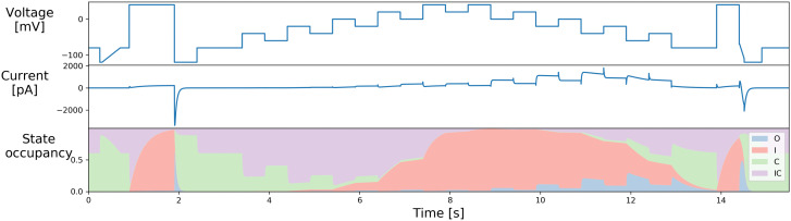 Figure 2
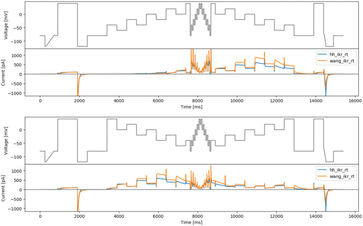 Figure 3
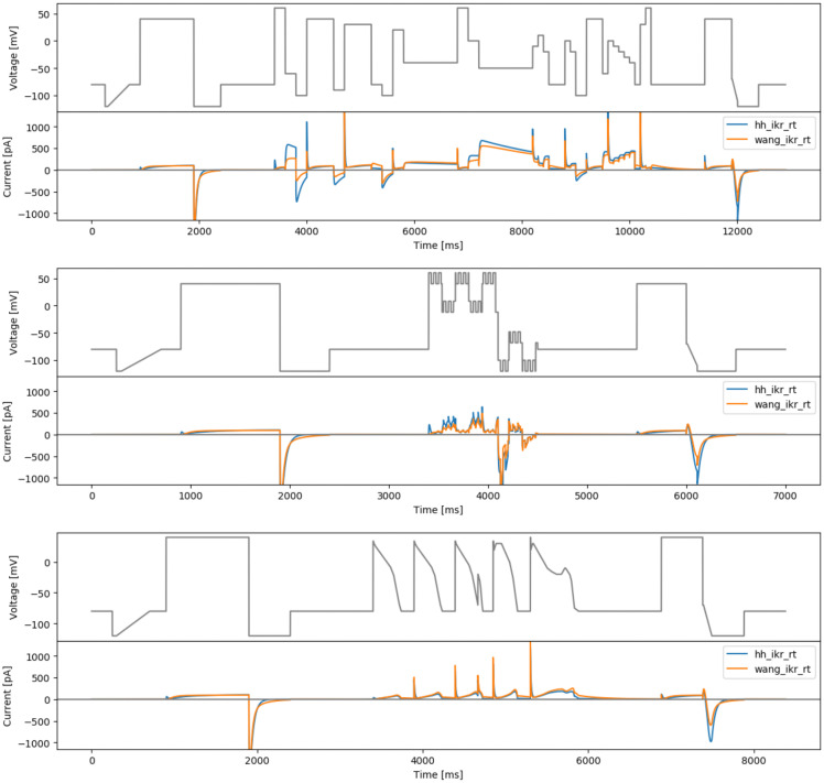 Figure 4
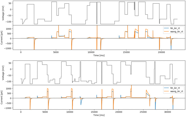 Figure 5
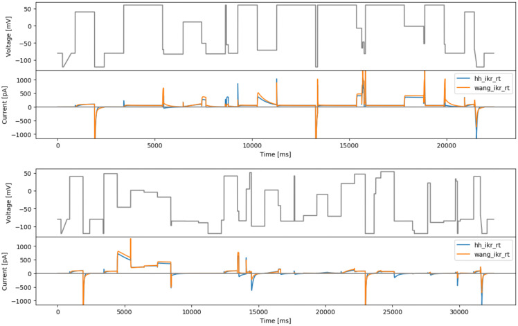 Figure 6
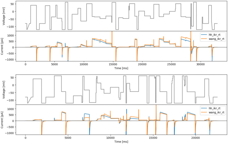 Figure 7
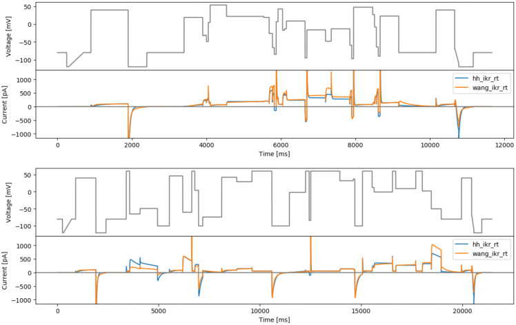 Figure 8
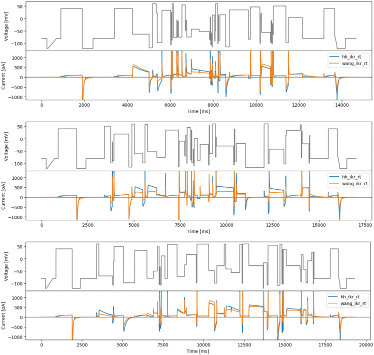 Figure 9
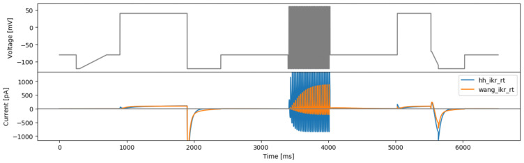 Figure 10
| Wang model | Beattie Model | ||||||
|---|---|---|---|---|---|---|---|
| Value | Range | Units | Value | Range | Units | ||
|
| 2.11 | — | ×10
–1
|
| 2.44 | — | ×10
–1
|
|
| 0.67 | [0.67,99993] | ×10 –2 ms –1 |
| 1.68 | [1.39,12.9] | ×10 –4 ms –1 |
|
| 1.31 | [1.31,99550] | ×10 –2 ms –1 |
| 8.06 | [1.08,8.49] | ×10 –2 mV –1 |
|
| 1.24 | [1.24,1.81] | ×10 –1 ms –1 |
| 4.34 | [2.77,32.3] | ×10 –5 ms –1 |
|
| 1.56 | [1.55,2.06] | ×10 –2 mV –1 |
| 4.07 | [2.48,4.56] | ×10 –2 mV –1 |
|
| 0.04 | [0.03,1.02] | ×10 –2 ms –1 |
| 9.07 | [6.40,19.9] | ×10 –2 ms –1 |
|
| 10.9 | [0.0001,10.9] | ×10 –2 mV –1 |
| 2.67 | [2.18,3.87] | ×10 –2 mV –1 |
|
| 0.24 | [0.23,364] | ×10 –2 ms –1 |
| 7.32 | [7.07,10.9] | ×10 –3 ms –1 |
|
| 0.0001 | [0.0001,6.44] | ×10 –2 mV –1 |
| 3.22 | [2.89,3.39] | ×10 –2 mV –1 |
|
| 3.15 | [1.29,7.69] | ×10 –4 ms –1 | ||||
|
| 3.99 | [2.97,3.99] | ×10 –2 mV –1 | ||||
|
| 5.75 | [3.55,5.75] | ×10 –3 ms –1 | ||||
|
| 2.89 | [2.89,3.34] | ×10 –2 mV –1 | ||||
|
| 0.28 | [0.007,1458] | ×10 –2 ms –1 | ||||
|
| 10.7 | [1.16,11.8] | ×10 –2 mV –1 | ||||
| Clamp | Initial: for leak and
| End: reversal ramp sequence | ||||
|---|---|---|---|---|---|---|
| # | Step/Ramp | t (ms) | V (mV) | Step/Ramp | t (ms) | V (mV) |
| 1 | Step | 250 | –80 | Step | 1000 | –80 |
| 2 | Step | 50 | –120 | Step | 500 | 40 |
| 3 | Ramp | 400 | –120 to –80 | Step | 10 | –70 |
| 4 | Step | 200 | –80 | Ramp | 100 | –70 to –110 |
| 5 | Step | 1000 | 40 | Step | 390 | –120 |
| 6 | Step | 500 | –120 | Step | 500 | –80 |
| 7 | Step | 1000 | –80 | — | — | — |
| Clamp | staircase | sis | sisi | manualppx | squarewave | |||||
|---|---|---|---|---|---|---|---|---|---|---|
| # | V (mV) | t (ms) | V (mV) | t (ms) | V (mV) | t (ms) | V (mV) | t (ms) | V (mV) | t (ms) |
| 1 | -40 | 500 | -40 | 500 | 40 | 500 | 60 | 200 | 60 | 24.9 |
| 2 | -60 | 500 | -60 | 500 | 0 | 500 | -60 | 200 | 40 | 25 |
| 3 | -20 | 500 | -20 | 500 | 20 | 500 | -100 | 200 | 60 | 25 |
| 4 | -40 | 500 | -40 | 500 | -20 | 500 | 40 | 500 | 40 | 25 |
| 5 | 0 | 500 | 0 | 500 | 0 | 500 | -90 | 200 | 60 | 25.1 |
| 6 | -20 | 500 | -20 | 500 | -40 | 500 | 30 | 500 | 40 | 9.9 |
| 7 | 20 | 500 | 20 | 500 | -20 | 500 | -80 | 200 | -12 | 15 |
| 8 | 0 | 500 | 0 | 500 | -60 | 500 | -100 | 200 | 8 | 25.1 |
| 9 | 40 | 500 | 40 | 225 | -40 | 225 | 20 | 200 | -12 | 24.9 |
| 10 | 20 | 500 | -80 | 50 | -80 | 50 | -40 | 1000 | 8 | 25 |
| 11 | 40 | 500 | -40 | 50 | -40 | 50 | 60 | 200 | -12 | 25.1 |
| 12 | 0 | 500 | -60 | 50 | -60 | 50 | 0 | 200 | 8 | 19.9 |
| 13 | 20 | 500 | -20 | 50 | -20 | 50 | -50 | 1000 | 60 | 5 |
| 14 | -20 | 500 | -40 | 50 | -40 | 50 | -10 | 100 | 40 | 25 |
| 15 | 0 | 500 | 0 | 50 | 0 | 50 | 10 | 100 | 60 | 25.1 |
| 16 | -40 | 500 | -20 | 50 | -20 | 50 | -20 | 100 | 40 | 25 |
| 17 | -20 | 500 | 20 | 50 | 20 | 50 | -80 | 300 | 60 | 25 |
| 18 | -60 | 500 | 0 | 50 | 0 | 50 | 0 | 100 | 40 | 24.9 |
| 19 | -40 | 500 | 40 | 50 | 40 | 50 | -20 | 100 | 60 | 5 |
| 20 | — | — | 20 | 50 | 20 | 50 | -100 | 200 | 8 | 20.1 |
| 21 | 40 | 50 | 40 | 50 | 40 | 300 | -12 | 24.9 | ||
| 22 | 0 | 50 | 0 | 50 | -60 | 100 | 8 | 25 | ||
| 23 | 20 | 50 | 20 | 50 | 0 | 100 | -12 | 25.1 | ||
| 24 | -20 | 50 | -20 | 50 | -10 | 100 | 8 | 24.9 | ||
| 25 | 0 | 50 | 0 | 50 | -20 | 100 | -12 | 15 | ||
| 26 | -40 | 50 | -40 | 50 | -30 | 100 | 40 | 10 | ||
| 27 | -20 | 50 | -20 | 50 | -40 | 100 | 60 | 25.1 | ||
| 28 | -60 | 50 | -60 | 50 | -80 | 100 | 40 | 24.9 | ||
| 29 | -40 | 50 | -40 | 50 | 30 | 100 | 60 | 25 | ||
| 30 | -80 | 50 | -80 | 50 | 60 | 100 | 40 | 25.1 | ||
| 31 | 40 | 225 | -40 | 225 | — | — | 60 | 24.9 | ||
| 32 | 0 | 500 | -60 | 500 | -12 | 25.1 | ||||
| 33 | 20 | 500 | -20 | 500 | -100 | 25 | ||||
| 34 | -20 | 500 | -40 | 500 | -120 | 25 | ||||
| 35 | 0 | 500 | 0 | 500 | -100 | 25 | ||||
| 36 | -40 | 500 | -20 | 500 | -120 | 24.9 | ||||
| 37 | -20 | 500 | 20 | 500 | -100 | 10 | ||||
| 38 | -60 | 500 | 0 | 500 | -48 | 15 | ||||
| 39 | -40 | 500 | 40 | 500 | -68 | 25.1 | ||||
| 40 | — | — | — | — | -48 | 25 | ||||
| 41 | -68 | 24.9 | ||||||||
| 42 | -48 | 25 | ||||||||
| 43 | -68 | 20 | ||||||||
| 44 | -120 | 5 | ||||||||
| 45 | -100 | 25 | ||||||||
| 46 | -120 | 25.1 | ||||||||
| 47 | -100 | 25 | ||||||||
| 48 | -120 | 24.9 | ||||||||
| 49 | -100 | 25.1 | ||||||||
| 50 | -120 | 4.9 | ||||||||
| 51 | -68 | 20 | ||||||||
| Clamp | rtovmaxdiff | maxdiff | longap | ||||
|---|---|---|---|---|---|---|---|
| # | V (mV) | t (ms) | V (mV) | t (ms) | Step/Ramp | V (mV) | t (ms) |
| 1 | 60 | 167 | -120 | 12.5 | Step | 34 | 3 |
| 2 | -65 | 516 | 60 | 12.5 | Ramp | 30 | 8 |
| 3 | -49 | 861 | -120 | 12.5 | Ramp | 26 | 15.2 |
| 4 | -100 | 587 | 60 | 12.5 | Ramp | -8 | 183.6 |
| 5 | 46 | 658 | -120 | 12.5 | Ramp | -21 | 39 |
| 6 | -60 | 446 | 60 | 12.5 | Ramp | -68 | 65.8 |
| 7 | 60 | 150 | -120 | 12.5 | Ramp | -80 | 25.2 |
| 8 | 4 | 185 | 60 | 12.5 | Step | -80 | 155.6 |
| 9 | -100 | 208 | -120 | 12.5 | Step | 34 | 3 |
| 10 | -74 | 935 | 60 | 12.5 | Ramp | 30 | 8 |
| 11 | 42 | 742 | -120 | 12.5 | Ramp | 26 | 15.2 |
| 12 | 29 | 751 | 60 | 12.5 | Ramp | -8 | 183.6 |
| 13 | 60 | 986 | -120 | 12.5 | Ramp | -21 | 39 |
| 14 | -100 | 866 | 60 | 12.5 | Ramp | -68 | 65.8 |
| 15 | -2 | 797 | -120 | 12.5 | Ramp | -80 | 25.2 |
| 16 | 60 | 177 | 60 | 12.5 | Step | -80 | 155.6 |
| 17 | -84 | 79 | -120 | 12.5 | Step | 34 | 3 |
| 18 | 60 | 943 | 60 | 12.5 | Ramp | 30 | 8 |
| 19 | 60 | 494 | -120 | 12.5 | Ramp | 26 | 15.2 |
| 20 | 32 | 666 | 60 | 12.5 | Ramp | -5 | 142.6 |
| 21 | 37 | 73 | -120 | 12.5 | Ramp | -21 | 38.4 |
| 22 | -100 | 380 | 60 | 12.5 | Ramp | -70 | 68.6 |
| 23 | 60 | 474 | -120 | 12.5 | Step | -20 | 2 |
| 24 | 12 | 101 | 60 | 12.5 | Ramp | -30 | 20 |
| 25 | -1 | 904 | -120 | 12.5 | Ramp | -40 | 10 |
| 26 | 60 | 162 | 60 | 12.5 | Ramp | -65 | 15 |
| 27 | 9 | 989 | -120 | 12.5 | Ramp | -80 | 12 |
| 28 | 60 | 323 | 60 | 12.5 | Step | -80 | 125 |
| 29 | 2 | 444 | -120 | 12.5 | Step | 34 | 3 |
| 30 | -50 | 492 | 60 | 12.5 | Ramp | 19 | 6 |
| 31 | — | — | -120 | 12.5 | Ramp | 30 | 26.4 |
| 32 | 60 | 12.5 | Step | 30 | 65 | ||
| 33 | -120 | 12.5 | Ramp | 0 | 99 | ||
| 34 | 60 | 12.5 | Ramp | -25 | 40 | ||
| 35 | -120 | 12.5 | Ramp | -80 | 55 | ||
| 36 | 60 | 12.5 | Step | -80 | 155 | ||
| 37 | -120 | 12.5 | Step | 40 | 3 | ||
| 38 | 60 | 12.5 | Step | 20 | 3 | ||
| 39 | -120 | 12.5 | Ramp | 30 | 20 | ||
| 40 | 60 | 12.5 | Step | 30 | 10 | ||
| 41 | -120 | 12.5 | Ramp | -10 | 168 | ||
| 42 | 60 | 12.5 | Ramp | -15.5 | 50.6 | ||
| 43 | -120 | 12.5 | Ramp | -20 | 61.2 | ||
| 44 | 60 | 12.5 | Step | -20 | 60 | ||
| 45 | -120 | 12.5 | Ramp | -10 | 40 | ||
| 46 | 60 | 12.5 | Step | -10 | 10 | ||
| 47 | -120 | 12.5 | Ramp | -20 | 50 | ||
| 48 | 60 | 12.5 | Ramp | -30 | 20 | ||
| 49 | -120 | 12.5 | Ramp | -75 | 36 | ||
| 50 | 60 | 12.5 | Ramp | -80 | 50 | ||
| Clamp | hh3step | wang3step | hhsobol3step | wangsobol3step | spacefill26 | |||||
|---|---|---|---|---|---|---|---|---|---|---|
| # | V (mV) | t (ms) | V (mV) | t (ms) | V (mV) | t (ms) | V (mV) | t (ms) | V (mV) | t (ms) |
| 1 | -96.7 | 983 | 59.8 | 1000 | 60 | 1000 | -120 | 52.8 | 40 | 841 |
| 2 | 59.7 | 730 | 35.3 | 1000 | 60 | 1000 | 48.2 | 1000 | -63 | 773 |
| 3 | -50.9 | 266 | -47.6 | 216 | -69.4 | 54.9 | -46.1 | 1000 | -117.9 | 163 |
| 4 | 9.07 | 852 | -107 | 341 | -82.5 | 999 | 1.3 | 1000 | 59.8 | 174 |
| 5 | 45.8 | 621 | -89.9 | 641 | 10.8 | 955 | -4.03 | 1000 | 22.1 | 46 |
| 6 | -45.5 | 360 | -80.7 | 377 | -51.1 | 219 | -17.8 | 1000 | -97 | 214 |
| 7 | -120 | 999 | -119 | 998 | -81.8 | 999 | -97.7 | 50.4 | 32.9 | 409 |
| 8 | -120 | 1000 | -74.6 | 281 | 60 | 51.5 | -85 | 784 | -106.1 | 29 |
| 9 | -88 | 222 | -60.4 | 54.4 | -55.4 | 103 | -85 | 232 | 25.1 | 20 |
| 10 | 30.2 | 388 | 59.8 | 1000 | -80.2 | 488 | -85.2 | 1000 | -86.8 | 23 |
| 11 | 56.6 | 972 | 28.3 | 1000 | 60 | 1000 | -89.8 | 711 | 59.9 | 56 |
| 12 | -120 | 50.2 | -47.8 | 233 | -71.1 | 1000 | -120 | 1000 | -76.9 | 156 |
| 13 | 57.5 | 497 | -111 | 61.2 | 60 | 1000 | -82.4 | 195 | -6 | 20 |
| 14 | -120 | 1000 | -99.2 | 398 | 60 | 1000 | 41.6 | 1000 | -74.3 | 37 |
| 15 | -120 | 999 | -78.7 | 116 | -120 | 102 | -57 | 108 | -10.6 | 20 |
| 16 | -96 | 642 | -102 | 783 | 60 | 1000 | -84.3 | 548 | -75 | 164 |
| 17 | 59.8 | 806 | -66.6 | 219 | 60 | 1000 | 5.02 | 261 | 55 | 160 |
| 18 | -42.5 | 400 | 60 | 151 | -7.19 | 269 | 51 | 129 | -47.5 | 25 |
| 19 | 56 | 936 | -97.6 | 443 | -64.9 | 50 | -99.5 | 1000 | -7.8 | 38 |
| 20 | -4.8 | 55.6 | -97.6 | 784 | -47.3 | 75.1 | 2.12 | 1000 | -74.4 | 213 |
| 21 | 59.8 | 50 | -107 | 317 | -81.4 | 67.3 | -41.7 | 187 | -42.7 | 367 |
| 22 | -53.1 | 488 | -95.3 | 665 | 60 | 1000 | -85.2 | 999 | -52.5 | 483 |
| 23 | 59 | 989 | -119 | 616 | 60 | 1000 | 41.9 | 50.2 | -85 | 33 |
| 24 | -42.8 | 321 | -111 | 407 | -1.7 | 1000 | -85.1 | 650 | 5.5 | 20 |
| 25 | -77.9 | 753 | 60 | 1000 | -52.4 | 50 | -69.6 | 1000 | -105.5 | 27 |
| 26 | 46.5 | 911 | -120 | 50 | 60 | 1000 | -10.2 | 815 | -58.6 | 32 |
| 27 | -116 | 54.3 | -120 | 50 | -54.1 | 50 | -71.5 | 1000 | -114.2 | 20 |
| 28 | — | — | 59.6 | 1000 | — | — | 20.3 | 1000 | 14.1 | 108 |
| 29 | 30.5 | 1000 | 46.8 | 797 | -90.5 | 20 | ||||
| 30 | -39.7 | 297 | -120 | 663 | -49.1 | 20 | ||||
| 31 | -120 | 725 | -8.4 | 128 | 59.9 | 103 | ||||
| 32 | -106 | 225 | 36.1 | 374 | -101.7 | 20 | ||||
| 33 | -108 | 568 | 53.8 | 999 | 15.1 | 20 | ||||
| 34 | 59.6 | 1000 | -85 | 949 | -87.8 | 61 | ||||
| 35 | 31.3 | 999 | -84.9 | 423 | 15.4 | 272 | ||||
| 36 | -41.9 | 187 | -111 | 129 | -114 | 169 | ||||
| 37 | 60 | 1000 | -120 | 1000 | 34.7 | 892 | ||||
| 38 | 60 | 1000 | 22 | 198 | -83.5 | 87 | ||||
| 39 | 60 | 1000 | -88.9 | 1000 | 46.6 | 444 | ||||
| 40 | -66.1 | 727 | -84.6 | 869 | -100.2 | 23 | ||||
| 41 | -120 | 931 | 33.6 | 50 | -3.3 | 23 | ||||
| 42 | 0 | 50 | 27.3 | 99.3 | 21 | 26 | ||||
| 43 | 60 | 159 | -120 | 50.3 | -55.8 | 421 | ||||
| 44 | -120 | 1000 | -85 | 107 | -95.3 | 29 | ||||
| 45 | -55.2 | 1000 | -85 | 60.7 | -8.4 | 32 | ||||
| 46 | — | — | — | — | -101.6 | 33 | ||||
| 47 | -20.7 | 20 | ||||||||
| 48 | -64.9 | 20 | ||||||||
| 49 | 50.5 | 585 | ||||||||
| 50 | -97.4 | 115 | ||||||||
| 51 | 3.7 | 658 | ||||||||
| Clamp | spacefill10 | spacefill19 | hhbrute3gstep | wangbrute3gstep | rvotmaxdiff | |||||
|---|---|---|---|---|---|---|---|---|---|---|
| # | V (mV) | t (ms) | V (mV) | t (ms) | V (mV) | t (ms) | V (mV) | t (ms) | V (mV) | t (ms) |
| 1 | 50.5 | 336 | 60 | 142 | 37.7 | 795 | 60 | 837 | 19 | 500 |
| 2 | -97.3 | 89 | -69.5 | 844 | -120 | 261 | -43.7 | 506 | -32 | 50 |
| 3 | -12.7 | 20 | -106.3 | 58 | -36.6 | 735 | -120 | 892 | -31 | 50 |
| 4 | -88.5 | 67 | -11.6 | 33 | 41 | 231 | -71.3 | 1000 | -49 | 50 |
| 5 | 18.8 | 804 | 48.8 | 584 | -45.3 | 815 | -117 | 50 | 5 | 50 |
| 6 | -114.3 | 166 | -97 | 689 | -65.4 | 50.2 | -114 | 50 | 54 | 439 |
| 7 | 59 | 149 | 33.6 | 752 | -120 | 530 | 57.9 | 169 | 22 | 499 |
| 8 | -60.5 | 438 | -79.1 | 398 | 60 | 459 | -33.4 | 617 | 22 | 500 |
| 9 | -97.5 | 120 | -49.8 | 257 | -120 | 714 | -116 | 757 | 19 | 145 |
| 10 | 57.5 | 144 | 50.5 | 99 | -19 | 1000 | -51.9 | 50 | -26 | 89 |
| 11 | -52.4 | 496 | -104.2 | 32 | 20.2 | 485 | 41.7 | 50 | -66 | 50 |
| 12 | -75 | 465 | -33 | 35 | -64.1 | 1000 | 57.2 | 50.4 | -85 | 50 |
| 13 | 34.7 | 711 | -106.3 | 62 | 50.4 | 947 | 12.8 | 446 | 7 | 50 |
| 14 | -113.5 | 31 | 11.5 | 228 | -34.1 | 362 | -28.6 | 358 | 43 | 121 |
| 15 | -9.7 | 299 | -79.6 | 153 | -36.5 | 991 | -55.2 | 746 | -17 | 53 |
| 16 | -70 | 33 | 58.2 | 594 | -47.3 | 1000 | -15.6 | 1000 | -13 | 50 |
| 17 | 12.2 | 79 | -71.3 | 462 | -30.8 | 1000 | -82.6 | 50 | 9 | 500 |
| 18 | -98.1 | 21 | -24.4 | 110 | -72.9 | 50.1 | -94.9 | 152 | -95 | 50 |
| 19 | 45.5 | 168 | 17.1 | 617 | 58.8 | 650 | -48.9 | 339 | -16 | 500 |
| 20 | -85.9 | 59 | -96.7 | 38 | -120 | 471 | 60 | 293 | -48 | 153 |
| 21 | 33.7 | 25 | 59.1 | 720 | -41.7 | 762 | -120 | 76.3 | -13 | 500 |
| 22 | -97.5 | 76 | -47.8 | 351 | -47 | 1000 | 10.8 | 363 | -59 | 50 |
| 23 | -42.7 | 32 | -98.5 | 151 | 35.4 | 50 | -27.8 | 50.5 | -97 | 50 |
| 24 | -109.7 | 21 | -28.1 | 457 | 8.1 | 50 | -43.6 | 1000 | 48 | 460 |
| 25 | 0.3 | 177 | 58.8 | 96 | 50.8 | 914 | 60 | 986 | 48 | 52 |
| 26 | -86.8 | 144 | -41.3 | 336 | -32.1 | 376 | -120 | 228 | 27 | 50 |
| 27 | -23.3 | 455 | -56.1 | 526 | -120 | 251 | 60 | 672 | -8 | 50 |
| 28 | -106.3 | 33 | 58.4 | 144 | -29.2 | 50 | 44.6 | 50 | -64 | 50 |
| 29 | 54.6 | 20 | -99.3 | 31 | 1.81 | 1000 | 49.8 | 50 | -90 | 50 |
| 30 | -60 | 169 | 59.8 | 382 | -30.1 | 1000 | -117 | 62.2 | 23 | 500 |
| 31 | 59.9 | 153 | -28 | 886 | -46.8 | 576 | 60 | 448 | — | — |
| 32 | -74.2 | 29 | -119.4 | 20 | 46.4 | 905 | -44.1 | 817 | ||
| 33 | 5.3 | 20 | -16.4 | 221 | -34.9 | 783 | -120 | 561 | ||
| 34 | -29.5 | 933 | -106.3 | 58 | -17.8 | 1000 | 9.6 | 50 | ||
| 35 | -105.9 | 35 | 54.5 | 586 | -0.1 | 1000 | 28.6 | 50 | ||
| 36 | 38 | 29 | -107.9 | 146 | 15.3 | 50 | 43 | 50.4 | ||
| 37 | -91.2 | 80 | 59 | 123 | 50.4 | 913 | 60 | 153 | ||
| 38 | -19 | 493 | -101 | 21 | -34.9 | 835 | -120 | 957 | ||
| 39 | -115.6 | 1007 | 37.2 | 20 | -38.9 | 818 | 60 | 206 | ||
| 40 | 59.9 | 218 | -102.3 | 46 | -116 | 50.5 | 32.1 | 50 | ||
| 41 | -99.5 | 54 | 37.7 | 182 | 50.5 | 115 | -7.3 | 50.5 | ||
| 42 | -42.1 | 799 | -27.8 | 849 | -98.1 | 324 | 1.1 | 50 | ||
| 43 | -101.5 | 105 | -43.9 | 44 | 60 | 512 | 58.9 | 200 | ||
| 44 | 14.5 | 36 | -93.5 | 37 | -120 | 980 | -45 | 947 | ||
| 45 | 33.7 | 754 | 16.7 | 107 | -37.1 | 98.9 | -120 | 105 | ||
| 46 | 56.3 | 45 | -42.7 | 179 | — | — | — | — | ||
| 47 | -75.8 | 25 | -97.3 | 102 | ||||||
| 48 | 28.7 | 26 | -8 | 250 | ||||||
| 49 | -20.5 | 364 | 26.4 | 93 | ||||||
| 50 | -98.9 | 26 | -101.3 | 20 | ||||||
| 51 | 13.1 | 21 | 26.8 | 27 | ||||||
- —University of Macau
- —Wellcome Trust
- —Engineering and Physical Sciences Research Council
- —Science and Technology Development Fund
- —Australian Research Council
Peer Reviews
No public reviews on file for this paper yet. If you reviewed it on a platform where reviews are public (OpenReview, ICLR, NeurIPS, ICML), you can paste yours below so the community can read it here.
Videos
No videos yet. Explain this paper in a talk, walkthrough, or lecture? Add one.
Taxonomy
TopicsCardiac electrophysiology and arrhythmias · Cardiac pacing and defibrillation studies · Neuroscience and Neural Engineering
Introduction
This report describes a series of voltage-clamp protocol waveforms that were designed to explore the gating of cell lines expressing hERG1a / K _v_11.1 channels, which are the primary subunit of the channels carrying the cardiac rapid delayed rectifier potassium current, I Kr ( Sanguinetti et al., 1995; Vandenberg et al., 2012).
The aim is to build on our previous studies that aimed to develop a range of short, information-rich voltage clamp protocols to use in experimental recordings to capture hERG gating behaviour ( Beattie et al., 2018; Lei et al., 2019b). Here we extend these to a wide range of protocols to better parameterise, select and test mathematical models of hERG gating ( Bett et al., 2011) and in particular to gain a better understanding and quantification of model discrepancy — when models cannot correctly predict what happens in reality ( Shuttleworth et al., 2024). As a result, some protocols will focus on classic optimal experimental design in terms of reducing uncertainty / improving identifiability of model parameter estimates ( Lei et al., 2023). Whilst others focus on maximising differences between trained models to assist in model selection/discrimination.
All these protocols were designed during the Isaac Newton Institute’s Fickle Heart programme in May–June 2019 ( Mirams et al., 2020). The protocols are all designed to be run on an automated patch platform, namely the Nanion SyncroPatch384PE ( Obergrussberger et al., 2016), which at the time had a restriction of only allowing up to 64 commands (steps or ramps) to define a single voltage-clamp protocol.
Models used in protocol design process
Our designs are model-driven akin to Lei et al. (2023), where mathematical models are used as part of automatic optimal design; even where our designs are manual they were done by visually examining the results of forward simulations.
The model structures that we used here are Beattie et al. (2018) and Wang et al. (1997) (also used in Fink et al. (2008)), with their Markov diagrams shown in Figure 1 and full equations reproduced below. The first model ( Beattie et al., 2018) is a Hodgkin-Huxley style model with two independent gates, which can be represented as a symmetric 4-state Markov model (see Fig. 4B of Rudy and Silva (2006)). The second model Wang et al. (1997) is a 5-state Markov model with 3 closed states, an open state, and an inactivated state connected sequentially.
The model structures used for experimental design.( a): the four-state Beattie et al. (2018) model. ( b): the five-state Wang et al. (1997) model. The arrows adjacent to each model structure indicate the direction in which rates increase as the voltage increases. Reproduced from Shuttleworth et al. (2024) under a CC-BY licence.
Beattie model
In matrix/vector form, the Beattie et al. (2018) model can be written as,
where
and
This model is equivalent to a two gate Hodgkin-Huxley style gating model with open probability given by an “activation” a gate representing the ‘right’ transitions in Figure 1a multiplied by an “inactivation” r gate representing the ‘down’ transitions ( Clerx et al., 2019a; Mirams, 2023), so in the below designs when we refer to “Hodgkin-Huxley” (HH) it is this interpretation of the model we are using.
Wang model
The Wang et al. (1997) model can be written as:
where
and
The default (room temperature) parameter values for both models are presented in Table 1. In practice we remove one state from the system and set it equal to “one minus the sum of the rest” to solve the ODE system, to improve numerical stability. All models are solved using a Python package Myokit ( Clerx et al., 2016) using SUNDIALS CVODE ( Hindmarsh et al., 2005).
Table 1.: The default parameter sets we use for the Wang et al. (1997) and Beattie et al. (2018) models.The column ‘Range’ indicates the parameter range obtained from real data fitting results based on protocols staircaseramp, sis, hh3step, and wang3step, which is used for global sensitivity-based designs.
Common protocol segments
As described in Mirams et al. (2024), all the protocols we have designed have common start and end sections, as defined in Table 2. The purposes of these sections are:
Table 2.: Details of the Start and End clamp sections for all designs.‘t’ indicates the duration of the clamp section, and ‘V’ the relevant voltage(s) for this clamp. Where ‘Ramp’ is specified it is a linear ramp over time between the voltages shown, as opposed to a constant voltage clamp for a ‘Step’. Reproduced from Mirams et al. (2024).
Start — an ‘activation step’ to provoke a very large tail current and help with conductance estimation, as discussed in Beattie et al. (2018).End — a ‘reversal ramp’ to help assess whether the current is reversing at the expected Nernst potential, discussed in Lei, Clerx, Gavaghan, et al. (2019b).both can also be used in quality control to check that these sections behave similarly over time when different protocols are applied to the same cell.
Manual protocol designs
The details of the protocols in this section are provided in Table 3.
**Table 3.: Details of the 5 protocols: staircase, sis, sisi, manualppx, and squarewave.All voltage values shown here are voltage steps to clamp to. These steps need to have the two ‘bookend’ sections added (see
Original staircase protocol
Figure 2 shows the original staircase protocol. It was manually designed to capture various dynamics of hERG ( Lei et al., 2019b; Lei et al., 2019a), which has been used and tested on the Nanion SyncroPatch384PE. We have been using it as a quality control of the full run of the experiments when designing the protocols in the rest of this report.
The manually-designed staircase protocol used in Lei, Clerx, Beattie, et al. (2019a; Lei et al., 2019b) and its simulation, with state occupancy shown for the Beattie et al. (2018) model of Figure 1a.Reproduced from ( Lei et al., 2019b) under a CC-BY licence.
Staircase-in-staircase protocol
The original staircase protocol provided a good foundation and motivation for improving experimental designs for characterisation of ion channel kinetics in high-throughput machines. We attempted to further improve this manual design by enhancing the exploration of inactivation processes of hERG. The original staircase protocol involves only voltage steps of 500 ms, which may not be able to explore fully the fast dynamics of hERG inactivation processes. Therefore, a shorter step duration version (50 ms) of the full staircase protocol is introduced at the middle of the staircase protocol, termed the staircase-in-staircase (sis) protocol ( Figure 3, top). We also explored the possibility of inverting the order of the staircase as shown in Figure 3, bottom (sisi).
Manual designs.Top: the staircase-in-staircase (sis) protocol. Bottom: the ‘inverted’ staircase-in-staircase (sisi) protocol. Underneath each protocol are simulated currents from the two models ( hh_ikr_rt is the Beattie et al. (2018) model of I Kr and wang_ikr_rt is the Wang et al. (1997) model of I Kr, both parameterised to room temperature data).
Phase-space filling protocol
The idea here is to have a protocol that fills up the phase-voltage space as much as possible. In brief, this design draws out the a, r, V three dimensional ‘phase-voltage space’ {[0,1],[0,1],[-120,60]} for the Beattie et al. (2018) model and subdivides it into 6 compartments in each dimension, giving a total of N = 6 ^3^ = 216 boxes. Since the phase space defines all possible behaviours of a model, if a protocol forces the model to visit as many of these boxes as possible, then the observations should test model assumptions well and provide rich information to fit model parameters. We have published the rationale and details of the design process for these protocol separately in Mirams et al. (2024). Figure 4 (top) shows a manually-tuned phase space filling protocol (manualppx); no objective function per se.
More manual designs.Top: the manual phase space protocol (manualppx). Middle: the square wave protocol of Beattie et al. (2018) (squarewave). Bottom: the lumped action potential protocol (longap). Beneath each protocol we show simulated currents from both the Beattie and Wang models.
A square-wave conversion of the sinusoidal protocol
In this design, we aim to design protocols based on sums of square waves, as inspired by Beattie et al. (2018). Such a protocol consists of a combination of N square waves, where each square wave i is defined by amplitude *a i *, (angular) frequency *ω i *, and phase lag *ϕ i *. The protocol is defined by 3 N parameters plus an extra parameter for an offset voltage, which can be expressed as:
where the function sign(⋅) takes a value +1 if its argument is positive, -1 if negative, or 0 if the argument is 0.
A direct conversion of the sine waves in the Beattie et al. (2018) protocol is performed, with the same amplitudes and frequencies, to square waves. It is a combination of three square waves ( N = 3) with a 1 = 54 mV, a 2 = 26 mV, a 3 = 10 mV, ω 1 = 0.007 ms, ω 2 = 0.037 ms, ω 1 = 0.19 ms, and ϕ 1 = ϕ 2 = ϕ 3 = 0, and an offset of b = −30 mV. The resulting protocol is called ‘squarewave’ and is shown in Figure 4 (middle).
Long action potential protocol
As a final ‘manually-chosen’ design, we also propose a lumped action potential protocol for validation purposes, as shown in Figure 4 (bottom). It consists of two action potential morphologies, an early after-depolarisation (EAD)-like action potential, and a delayed after-depolarisation (DAD)-like action potential. The details of this longap protocol are provided in Table 4.
**Table 4.: Details of the 3 protocols: rtovmaxdiff, maxdiff, and longap.All voltage values for protocols rtovmaxdiff and maxdiff are voltage steps to clamp to. Protocol longap also indicates with ‘Ramp’ or ‘Step’; ‘Ramp’ is specified it is a linear ramp over time between the voltages shown, as opposed to a constant voltage clamp for a ‘Step’. These steps need to have the two ‘bookend’ sections added (see
Automated Iterative 3-step designs
Here we describe protocol design approaches that can be done objectively and automatically. With the same rationale as described in Mirams et al. (2024), we consider a protocol consists of 3 N steps with N ∈ ℕ, and we split the protocol into N units with 3 consecutive voltage steps as a unit. For some designs, N is the number of model parameters, while for others, N is 17 to bring the total number of steps to 51 which is close to the 64 allowed by the Nanion SyncroPatch384PE when the start and end clamps are added ( Table 2). For each unit i, we optimise the 3 voltage steps through an objective function *S i *, with each step defined by two parameters: voltage V and duration Δt. Each objective function *S i
- (described in the sections below) aims to achieve a different purpose. We then iterate the process for all the objective functions i = 1, 2, … N, resulting in a 3 N steps protocol.
The optimisation was performed using a global optimisation scheme, covariance matrix adaptation evolution strategy (CMA-ES, Hansen, 2006) implemented via a Python package PINTS ( Clerx et al., 2019b). All optimisation of the designs were repeated 10 times from different randomly varied initial starting points, and the best designs are presented here. Although we do not expect our design would reach the same global optimum as optimising all > 20 steps at once ( Mirams et al., 2024), our results still show promising protocol designs. We also tried to perform fitting 6-steps-at-once in Mirams et al. (2024) and showed that both resulted in similar performance. Finally, the presented results are the optimised results rounded to the nearest one decimal place in millisecond and millivolt for practical implementation ( Mirams et al., 2024).
The details of the protocols in this section are provided in Table 4, Table 5 and Table 6.
**Table 5.: Details of the 5 protocols: hh3step, wang3step, hhsobol3step, wangsobol3step, and spacefill26.All voltage values shown here are voltage steps to clamp to. These steps need to have the two ‘bookend’ sections added (see
**Table 6.: Details of the 5 protocols: spacefill10, spacefill19, hhbrute3gstep, wangbrute3gstep, and rvotmaxdiff.All voltage values shown here are voltage steps to clamp to. These steps need to have the two ‘bookend’ sections added (see
Sensitivity-based designs
** Maximising approximated local sensitivity **
For an ion channel current model I with N parameters p 1, p 2, ... *p N *, we define an objective function for each 3-step unit i that maximises the absolute value of the sensitivity of the model output I with respect to the parameter *p i
- while minimising all the absolute value of sensitivity of the rest of the parameters. This objective function can be mathematically expressed as
The sensitivity was calculated using a first-order central difference scheme with δ *p i
- being 0.1 % × *p i *. Note that the integration is only over the last step of the 3 steps, the idea is to allow the first two steps to vary as much as it would need to be to maximise the approximated local sensitivity across the third step (it is fine if there is low sensitivity because of e.g. full inactivation in the first two steps). This has been repeated for both models and the results are shown in Figure 5.
The 3-step local sensitivity designs.Top: protocol based on the Hodgkin-Huxley model (hh3step). Bottom: based on the Wang model (wang3step). With simulated currents from both models shown below the protocols.
** Maximising Sobol sensitivity **
Instead of the local sensitivity, we can also replace it with the first-order Sobol global sensitivity indices, given by
Here the *p !i
- notation denotes the set of all parameters except *p i *. This has been repeated for the Beattie & Wang models. The parameter range ( Table 1) was taken from previous real data fits to staircaseramp, sis, hh3step and wang3step, using the approach from Lei, Clerx, Gavaghan, et al. (2019b) without accounting for experimental error ( Lei et al., 2020a; Lei et al., 2020b).
To calculate Sobol sensitivities we used a modified version of the SA-lib library ( Herman & Usher, 2017), to enable easier calculation of sensitivities over time series, which is included in our repository (see Data Availability). The results are shown in Figure 6.
The 3-step Sobol sensitivity protocols.Top: based on the Hodgkin-Huxley model (hhsobol3step). Bottom: based on the Wang model (wangsobol3step). With simulated currents from both models shown below the protocols.
Gibbs designs
We use the 3-step approach discussed above, but the difference here is that instead of defining each step by two parameters (voltage V and duration Δt), for each 3-step section we optimise only one of these parameters (either V or Δt) while randomly picking the other from a uniform distribution. This halves the number of parameters that are inferred to just 3 per 3-step section. However, since we have only the same objective function, all units would return the same optimum (or a few if multi-modal but very limited) which is not desired. Therefore we introduce some stochasticity to the protocol by randomly choosing one of the step parameters and optimising only the other one.
** Maximising model output differences: a brute-force sampling approach **
The approach taken in this design is similar to a global sensitivity analysis. For a given model I, we start with randomly picking M (ideally ∼ 1000s but practically ∼ 100s of) parameters from model parameter prior, then the objective function to be optimised is the sum of the root mean square deviation (RMSD) values between the model outputs from all combinations of the sampled parameter pairs. The model parameter prior could be an a-priori distribution of the parameters (for example those used in Beattie et al., 2018; Lei et al., 2019b), or based on previous fitting results (see below). The objective function for a 3-step unit i can be expressed as
where RMSD( x, y) denotes the RMSD between x and y, and *I j *, *I k
- are the model output for the M parameter samples. We choose θ
i
- = with *Δt j
- ∼ Uniform(50,1000) ms for odd i, and θ
i
- = with *V j
- ∼ Uniform(–120,60) mV for even i.
This has been repeated for the Beattie and Wang models, with the parameter range (prior distribution) was taken from the extremes of the range defined by previous real data fits to staircsaeramp, sis, hh3step and wang3step, as provided in Table 1. The results are shown in Figure 7.
The brute-force sampling protocols.Top: based on the Hodgkin-Huxley model (hhbrute3gstep). Bottom: based on the Wang model (wangbrute3gstep). Simulated currents from both models are shown beneath each protocol.
** Maximising differences between two models **
Unlike the previously defined approaches, where only one model was involved, this proposed approach aims to distinguish between two candidate models. The objective function is defined as the RMSD value between two model currents, with a given set of model parameters ( Table 1), so it is still a ‘local’ design with respect to model parameters. One protocol randomly picks time parameters for each 3-step unit, and optimises voltages with *Δt j
- ∼ Uniform(50,500) ms and is termed ‘rtovmaxdiff’); and the other method randomly picks voltages and optimises the step durations with *V j
- ∼ Uniform(–120,60) mV, and is known as ‘rvotmaxdiff’. Applying this approach to the Beattie & Wang models results in Figure 8.
Protocols that maximise the difference between currents from the Beattie and Wang models.Top: based on randomised voltage and optimising time steps (rvotmaxdiff). Bottom: based on randomised time steps and optimised voltages (rtovmaxdiff). Simulated currents from both models are shown beneath each protocol.
Phase-voltage space filling designs
For details of this approach, see Mirams et al. (2024). Briefly, an objective function tries to maximise the amount of new boxes that are visited by a model’s trajectory for each new iterative ‘3 step’ set of pulses (as described above) repeating sequentially until we have 17 sets of 3 steps. This approach has a stochastic optimisation step, and produces some protocols that appear to be challenging and information rich, where we appear to have a reasonable amount of current and interesting dynamics. After 30 optimisation runs with different random seeds and initial guesses, we selected the following 3 best protocols based on slightly different criteria:
Figure 9, top — Number 26: the best space-filling objective function score ( Mirams et al., 2024). Figure 9, middle — Number 10: the largest RMSD value between the two models’ simulated currents. Figure 9, bottom — Number 19: the best brute-force sampling score ( Eq. (2)) for the Beattie et al. (2018) model.
Phase-voltage space filling designs.Top: first phase-voltage space protocol (spacefill26). Middle: second phase-voltage space protocol (spacefill10). Bottom: third phase-voltage space protocol (spacefill19), with simulated currents from both models.
All three protocols visit between 126–132 (58–61%) of the available 216 ‘boxes’ in phase-voltage space. Note that this is a lower percentage than the protocols in Mirams et al. (2024) primarily due to 1 ms time samples being used in the 2019 optimisations presented here (see Discussion of Mirams et al. (2024)) along with extra initial guesses now being used in the Mirams et al. (2024) optimisation procedure to gain slightly higher coverage of the space.
Automated square waves
Following the same argument as in ‘Maximising differences between two models’ above, this design maximises the differences between two candidate models to aid model selection. Here we use N = 3 (as per Beattie et al., 2018) which gives 9 parameters in total (see Equation (1)), with a fixed offset voltage of −30 mV. The square wave parameters are optimised based on an objective function that maximises the RMSD value between two model outputs. As above, the two models have a set of predefined model parameters, so it is still a ‘local’ model parameter method.
This approach was applied to the Beattie and Wang models using their original literature parameters. The resulting protocol ( Figure 10) exhibits extremely high frequency and high amplitude (hitting the boundaries of the protocol parameters) behaviour. We believe these rapid changes of voltage tends to maximise the two model outputs, which is similar to the ‘original sine wave #2’ in Beattie (2015), and is likely to be impractical or uninformative for real experiments.
The square wave protocol for maximising two models’ difference (maxdiff) and simulated currents from both models.
Discussion
Developing ion channel models remains a challenging task predominantly due to all the various sources of uncertainty and variability ( Mirams et al., 2016) — in terms of modelling approximations ( Lei et al., 2020c; Lei & Mirams, 2021) as well as experimental noise and artefacts ( Lei et al., 2020a). It is made more difficult due to the sparsity of available data for independent training and validation, with it still being common to calibrate models to all available data ( Whittaker et al., 2020). The protocols presented here encompass many design criteria, including parameterisation, model selection and rigorous testing of the underlying assumptions in hERG models ( Fink & Noble, 2009; Lei et al., 2019b; Mirams et al., 2024). As such, we expect that this collection of voltage clamp protocols will be extremely useful for development of mathematical models for the physiological gating of the hERG potassium channel, and in particular by providing ample validation data for assessing their prediction errors due to model discrepancy ( Shuttleworth et al., 2024).
The same design criteria we have outlined here could easily be applied to other ion channels to create similar suites of protocols, using the provided open source codes.
Ethics and consent
Ethical approval and consent were not required.
The reference list from the paper itself. Each links out to its DOI / PubMed record.
- 1Beattie K : Mathematical modelling of drug-ion channel interactions for cardiac safety assessment.Ph D thesis, University of Oxford,2015. Reference Source
- 2Beattie KA Hill AP Bardenet R : Sinusoidal voltage protocols for rapid characterisation of ion channel kinetics. J Physiol. 2018;596(10):1813–1828. 10.1113/JP 275733 29573276 PMC 5978315 · doi ↗ · pubmed ↗
- 3Bett GCL Zhou Q Rasmusson RL : Models of HERG gating. Biophys J. 2011;101(3):631–42. 10.1016/j.bpj.2011.06.050 21806931 PMC 3145286 · doi ↗ · pubmed ↗
- 4Clerx M Beattie KA Gavaghan DJ : Four ways to fit an ion channel model. Biophys J. 2019 a;117(12):2420–2437. 10.1016/j.bpj.2019.08.001 31493859 PMC 6990153 · doi ↗ · pubmed ↗
- 5Clerx M Collins P De Lange E : Myokit: a simple interface to cardiac cellular electrophysiology. Prog Biophys Mol Biol. 2016;120(1–3):100–114. 10.1016/j.pbiomolbio.2015.12.008 26721671 · doi ↗ · pubmed ↗
- 6Clerx M Robinson M Lambert B : Probabilistic Inference on Noisy Time Series (PINTS). J Open Res Softw. 2019 b;7(1): 23. 10.5334/jors.252 · doi ↗
- 7Fink M Noble D : Markov Models for ion channels: versatility versus identifiability and speed. Philos Trans A Math Phys Eng Sci. 2009;367(1896):2161–79. 10.1098/rsta.2008.0301 19414451 · doi ↗ · pubmed ↗
- 8Fink M Noble D Virag L : Contributions of h ERG K + current to repolarization of the human ventricular action potential. Prog Biophys Mol Biol. 2008;96(1–3):357–76. 10.1016/j.pbiomolbio.2007.07.011 17919688 · doi ↗ · pubmed ↗