Joint Modeling of Longitudinal Visual Field Changes and Time to Detect Progression in Glaucoma Patients: A Secondary Data Analysis

TL;DR

This study uses a Bayesian model to analyze how visual field changes and disease progression are linked in glaucoma patients over time.

Contribution

The novelty is the use of a Bayesian joint model to integrate longitudinal visual field data with progression risk in glaucoma.

Findings

Older age, higher intraocular pressure, and early-stage disease were significantly linked to increased progression risk.

Longitudinal mean deviation changes were strongly associated with progression risk (α=-0.39, P<0.001).

Sex was not found to significantly influence glaucoma progression.

Abstract

Glaucoma causes irreversible damage to the optic nerve and can lead to blindness if it is not treated appropriately. Evaluation of longitudinal changes in the visual field (VF) and detecting progression in a timely manner are critical for effective disease management. This study aimed to identify factors associated with VF impairment and disease progression using a Bayesian joint model.

A total of 129 glaucoma patients (228 eyes) were recruited from an ongoing cohort study initiated in 1998 at the Rotterdam Eye Hospital in the Netherlands. Standard Automated Perimetry (SAP) was performed for each patient at regular 6-month follow-up intervals. Covariates included sex, age at baseline, mean intraocular pressure (IOP), and disease severity. A Bayesian joint model was employed, integrating a linear mixed effects model (LMM) for longitudinal mean deviation (MD) values and a Cox proportional hazards model for progression time. The statistical analyses were conducted using R software and the ‘JMbayes2’ package.

Progression was observed in 33.8% of eyes. A significant association was found between MD changes and progression risk (α=-0.39, P<0.001). Older age (P=0.01), early-stage disease (P<0.001), and higher mean IOP (P<0.001) were associated with an increased risk of progression.

Considering longitudinal MD changes, age at baseline, mean IOP, and disease severity were significantly associated with the time to progression detection. Sex was not found to be a significant factor in glaucoma progression.

Figures

The figure represents the density plot for the values of mean deviation (MD).

Tables

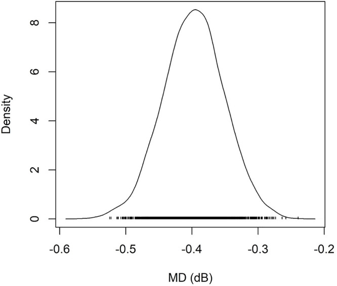Table 1. Demographic characteristics of glaucoma patients

Variables		Value n (%)/mean±SD
Age (years)		59.71±10.18
Follow-up (years)		9.02±1.21
Number of tests per eye		17.42±2.50
Baseline MD (dB)		-6.93±5.13
Mean IOP (mmHg)		14.68±2.94
Sex	Male	73 (56.59)
	Female	56 (43.41)
Disease severity	Mild	122 (53.51)
	Moderate	61 (26.75)
	Severe	45 (19.74)

Table 2. Comparison of LMM with different random terms

Model	AIC	BIC	Log-likelihood
Random intercept	12889.21	12920.04	-6439.60
Random slope	13648.00	13678.83	-6818.99
Random intercept and slope	12746.13	12789.30	-6366.06

Table 3. Summary of joint model results

Models	Variables		Estimate (β)	SE	P value	Hazard Ratio (hi)
Cox PH model	Age at Baseline (Year)		0.033	0.013	0.014	1.033
	Mean IOP (mm Hg)		0.173	0.045	<0.001	1.188
	Sex	Female	-	-	-	-
		Male	-0.526	0.326	0.106	0.590
	Disease severity	Early	-	-	-	-
		Moderate	-1.905	0.388	<0.001	0.148
		Severe	-4.773	0.675	<0.001	0.008
	Associate parameter		-0.397	0.046	<0.001	0.672
LMM	Time (Year)		-0.103	0.023	<0.001
	Age at Baseline (Year)		0.001	0.013	0.963
	Mean IOP (mm Hg)		0.158	0.047	<0.001
	Sex	Female	-	-	-
		Male	0.031	0.277	0.911
	Disease severity	Early	-	-	-
		Moderate	-5.277	0.334	<0.001
		Severe	-12.082	0.379	<0.001
	Random effects	Random	Standard deviation
		Intercept	1.987
		Slope	0.304
		Correlation	0.217

Full text

What’s Known

• Assessing longitudinal visual field changes enables clinicians to detect disease progression in glaucoma patients.
• Typically, linear mixed-effects models or Cox regression are used to analyze glaucoma data and identify factors associated with visual field deterioration, or the time to progression detection.

What’s New

• The effect of various risk factors on progression detection was evaluated using a joint model. The findings of the present study indicated an inverse association between the risk of progression and mean deviation values.
• Older age, higher mean intraocular pressure (IOP), and early-stage disease were identified as factors associated with an increased risk of progression.

Introduction

Glaucoma is a chronic condition that causes irreversible damage to the optic nerve and can lead to blindness if not treated appropriately. ^ 1 , 2 ^ It typically affects individuals aged 40-80 years, and it is predicted that by 2040, approximately 112 million people worldwide will be affected by the disease. ^ 3 ^ Glaucoma imposes a significant financial burden on patients and society, including both direct and indirect costs, with disease severity. ^ 4 , 5 ^ Additionally, the gradual loss of vision associated with glaucoma adversely affects patients’ daily activities. Therefore, understanding the spectrum of the disease is essential for adjusting treatment plans in cases of disease progression. ^ 1 , 6

• 8 ^

Mean deviation (MD) reflects the overall loss in visual field (VF) sensitivity. ^ 9 ^ Evaluating longitudinal changes in MD may assist in distinguishing true progression from noise in VF measurements. ^ 10 ^ In addition, it is important to determine the factors associated with rapid progression in glaucoma patients. Some clinical factors, such as severity of VF impairment and age were reported to be related to an increased risk of progression. ^ 11

• 13 ^ Numerous randomized controlled trials (RCTs) highlighted the reduction of intraocular pressure (IOP) as a primary treatment to prevent progression. ^ 14
• 16 ^

Glaucoma patients require regular monitoring to adjust treatment if progression is detected. ^ 17 ^ In addition to longitudinal measurements of MD over time, the time point at which progression is flagged (time-to-event) can be determined. The criterion for detecting progression was described in a previous study. ^ 17 ^ Consequently, there would be two types of outcomes in such analyses. Classical statistical tools often model these outcomes separately, failing to account for the relationship between the two response variables. This approach may lead to inaccurate or biased inferences. Joint models have been developed to simultaneously analyze both repeated measures and time-to-event data. These models are particularly beneficial when the study aims to identify associations between longitudinal follow-up data and event times. ^ 18 ^

Previous studies have paid limited attention to simultaneously modeling longitudinal VF changes and time to detect progression in glaucoma patients. ^ 11

• 13 ^ To address this gap, this study aimed to identify factors associated with VF impairment and progression time using a Bayesian joint model with a Markov chain Monte Carlo (MCMC) algorithm.

Patients and Methods

Participants in this study were recruited from an ongoing cohort study initiated in 1998 at the Rotterdam Eye Hospital in the Netherlands. The study received ethical approval from the Institutional Review Board at the Rotterdam Eye Hospital, and all participants provided written informed consent. ^ 19 ^ The Rotterdam Ophthalmic Institute (ROI) has made certain anonymized datasets related to eye measurements publicly available to facilitate scientific research. These datasets are provided free of charge under a License Agreement and can be accessed online at www.rodrep.com. This study was also approved by the Ethics Committee of Shiraz University of Medical Sciences (Shiraz, Iran), code: IR.SUMS.REC.1400.082.

Glaucoma was diagnosed based on the following criteria: pattern standard deviation significant at P=0.05, an abnormal hemifield test result, or a cluster of ≥3 points depressed at P=0.05 level or 1 point at P=0.01. Only glaucoma patients with open-angle eyes were included in this study. Standard Automated Perimetry (SAP) VF tests were conducted for patients aged 18-85 years old at 6-month intervals. The tests were conducted using Humphrey Visual Field Analyzers (Carl Zeiss Meditec, Dublin, CA) with a standard white-on-white 24-2 field and the full threshold program. Age at baseline, sex, and IOP were recorded for each patient. ^ 19 ^ Mean IOP was calculated for each eye over time. Disease severity was determined based on the initial mean deviation (MD), with eyes classified as having early (MD between 0 and -6 dB), moderate (MD between -6 and -12 dB), or severe (MD between -12 and -20 dB) glaucoma. ^ 20 ^

Progression time was the primary outcome of interest in this study. MD values were measured every 6 months using the SAP VF tests. At each visit, an ordinary least-squares regression model was fitted on MD values measured from the baseline for each eye. Progression was flagged if the rate of progression was negative (Slope<0), and the P<0.05 was statistically significant in two successive visits. ^ 17 ^ The time of progression detection was then recorded.

Statistical Analysis

For each eye, the time point at which the progression criteria were met was recorded. The survival time (in years) was defined as the duration between the start date of monitoring and the date of progression (or censoring). In addition, MD values were recorded every 6 months for each eye. Given the presence of two types of response variables in this study, joint analysis was employed to simultaneously model longitudinal changes in MD and time to progression detection in glaucoma patients. ^ 18 ^ The joint model links survival and longitudinal sub-models through a shared random parameter.

The Survival Sub-model

Survival analysis is a branch of statistical methods that deals with time-to-event data. Let T represent the time when progression occurs in glaucoma patients. The survival function, S(t)=P(T>t), denotes the probability of survival for an individual beyond time t. The notation T_i_ represents the true time-to-event for the subject i, and C_i_ represents the corresponding censoring time. The event indicator (δi=I[Ti≤Ci]) takes the value 1 if an event occurs (if Ti≤Ci) and 0 if the observation is censored (if Ti>Ci).

The Cox proportional hazards (PH) model is a semi-parametric approach widely used for survival analysis. This model investigates the effect of multiple variables on the time until an event occurs. The hazard function at time t is expressed as follows:

hi(t)=h0(t)exp(βTXi) (1)

Where β is a vector of coefficients for independent variables X_i_. The coefficients are related to the hazard and indicate the prognosis of the disease. The hazard of progression for the i^th^ individual at time t is denoted by h_i_(t), and h_0_(t) represents the baseline hazard function. Since the model is based on the assumption of proportional hazards, graphical evaluation of Kaplan-Meier curves, log (-log [survival]) plots, or Schoenfeld residuals should be used to verify this assumption for predictors. ^ 18 , 21 ^

The Longitudinal Sub-model

In longitudinal studies, measurements for an individual change over time, and there is variation between the subjects due to patient-specific characteristics (subject-specific effects). A linear mixed effects model (LMM) is typically used to analyze longitudinal data, accounting for the correlation between repeated measurements. LMM includes both fixed and random effects to evaluate continuous longitudinal data. Fixed effects assume that variables have constant impacts on the response variable across all cases, while random effects account for variability across the subjects. Subject-specific effects are random terms that account for correlation among the repeated observations for each subject. The LMM is generally expressed as follows:

{Yi=Xiβ++Zibi+εi,biN(0,σb2),εiN(0,σ2I),biandεiareindependent , (2)

where β denotes coefficients for fixed effects, and b_i_ indicates subject-specific effects. The design matrices of X_i_ and Z_i_ link the fixed and random effects to longitudinal measurements of Y_i_. The notation ε_i_ denotes random errors. Random terms of b_i_ and ε_i_ are assumed to be independent, and typically follow a normal distribution. ^ 18 , 22 ^

The Joint Model

The joint model examines the association between longitudinal and survival data using a shared random effect. Meanwhile, it considers the correlation between repeated measurements. The shared random parameter model can be written as follows:

hi(t|Mi(t))=h0(t)exp(γTwi+αmi(t)) (3)

where M_i_ (t)=(m_i_(s), 0≤s<t) represents the history of the unobserved longitudinal response up to time t. The baseline covariates are denoted by W_i_ with parameter γ; and α quantifies the effect of the longitudinal outcome on the risk of an event. ^ 18 ^

In glaucoma data, correlations exist between pairs of repeated MD measurements. Therefore, based on the nature of the data and according to a previous study, ^ 23 ^ a continuous first-order autoregressive (AR(1)) structure was used for the correlation structure in the LMM. The AR(1) model assumes that the value of MD at time t depends on its value at time t-1. Three models with different random terms (random intercept, random slope, and random intercept and slope) were fitted. The best LMM was selected based on the minimum values of the Akaike information criterion (AIC) and Bayesian Information Criterion (BIC), as well as the maximum log-likelihood value. Covariates investigated in this study included age at baseline, sex, mean IOP, and disease severity (mild, moderate, and severe) at baseline. Initially, multivariate LMM and Cox PH regression were fitted separately. The proportional hazard assumption was verified using Schoenfeld residuals. Subsequently, joint modeling of survival and longitudinal data was performed using the JMbayes2 package in R software (R Core Team, Austria; version: 4.0.2). ^ 24 ^ Model parameters were estimated using the MCMC approach with Gibbs sampling. The convergence of the models and the stationary distribution of the chains were assessed using diagnostic plots. ^ 25 ^

Results

A total of 129 glaucoma patients (228 eyes) were included in this study. Progression occurred in 77 eyes (33.8%), with a mean time to progression (95% confidence interval=6.0 [5.4-6.5]) years. The mean±SD age of the patients at the baseline was 59.7±10.2 years. There were 6 to 21 visits available per eye, with an average of 17.2±2.5 visits. Baseline MD was -6.9±5.1 dB (median=-5.6 dB, Interquartile range=8 dB), and nearly half of all patients (53.5%) were in the early stage of the disease at baseline. The demographic characteristics of the patients are summarized in table 1.

LMMs with different random terms were fitted. The LMM with random intercept and slope, which resulted in the lowest AIC and BIC values as well as the maximum Log-likelihood, was selected (table 2). Subsequently, multivariate analysis was conducted using a linear mixed effects model and Cox proportional hazard regression.

To investigate the association between the longitudinal and survival responses in the glaucoma data, a joint model with a shared random parameter was fitted (table 3). The longitudinal sub-model revealed that time (P<0.001), mean IOP (P<0.001), and disease severity (P<0.001) were significantly associated with changes in MD over time. In the survival sub-model, mean IOP (P<0.001), age at baseline (P=0.01), and disease severity (P<0.001) were statistically significant. Older age at baseline and a higher mean IOP were associated with an increased risk of progression. Furthermore, patients with early-stage glaucoma had a higher risk of progression than those with moderate and severe glaucoma.

The association parameter indicated a significant association between MD changes and the time to progression (P<0.001) in glaucoma patients. The negative value of the association parameter indicated a reverse association between the risk of disease progression and MD values. Convergence of Markov chains was assessed using diagnostic plots for all parameters. Figure 1 provides an example of the density plot for the association parameter. The density plot demonstrated that the posterior marginal distribution had converged to the target distribution, as evidenced by its uni-modal and smooth shape.

The figure represents the density plot for the values of mean deviation (MD).

Discussion

In this study, we applied a joint modeling approach using LMM and Cox regression to analyze longitudinal VF measures and progression time in glaucoma patients. The findings revealed a significant association between these two outcomes through a shred random parameter in the Bayesian joint model. Age at baseline, mean IOP, and disease severity were significantly associated with progression time.

To investigate the functional performance of a patient’s VF, MD was measured at each clinical visit to monitor vision loss and glaucoma progression. ^ 10 ^ It is critical to evaluate how MD changes were related to the risk of progression. Furthermore, several factors were found to have an impact on VF changes, including IOP, which was the only controllable factor for preventing progression in glaucoma patients. ^ 12 , 13 , 26 ^

The joint model enables the identification of major disease risk factors, as well as the association between longitudinal MD changes and the progression time in glaucoma patients. ^ 18 ^ As previously established, the joint model improves the survival model by incorporating random effects from longitudinal measurements. This approach enhances the precision of parameter estimations by considering the correlation between survival and longitudinal outcomes, which is often overlooked in individual modeling. ^ 27 ^ Moreover, the linear mixed effects model adjusts for non-ignorable missing data due to informative withdrawal by incorporating time-to-event data. ^ 28 ^

Up to now, numerous studies have investigated the role of sex in glaucoma development and its impact on disease progression. ^ 29

• 32 ^ While men were thought to carry a heavier global burden of glaucoma, ^ 29 ^ a different study reported a higher prevalence of glaucoma among women. ^ 30 ^ Additionally, a study found that lower estrogen levels were associated with glaucoma progression in premenopausal women. ^ 31 ^ In the current study, there was no significant difference in the number of men and women participants. The joint model did not identify sex as a significant factor for disease progression. This finding was consistent with previous studies that failed to identify sex as a significant risk factor for rapid VF progression. ^ 11 , 26 ^

Our findings indicated that a one-year increase in the variable time was associated with a 0.1 dB decrease in MD. Although age at baseline was not significant in the LMM sub-model, it was identified as a risk factor for progression in the survival sub-model. For each 5-year increment in baseline age, the risk of the disease progression increased by 15%. Age is known as an important non-modifiable risk factor for glaucoma prevalence. ^ 33 , 34 ^ Previous studies found an association between getting older and having a faster progression in patients with glaucoma. ^ 26 , 35 ^ Older patients might probably be more susceptible to MD changes and glaucoma progression due to a smaller neural reserve. ^ 35 ^

In the present study, mean IOP was significantly associated with both MD changes and time to detect progression. For each 1-mm Hg increase in mean IOP, the risk of progression increased by 18%. This finding was in line with previous studies suggesting that a lower IOP slowed down VF deterioration. ^ 33 , 36 ^ However, the role of IOP in glaucoma progression remains controversial. ^ 13 , 37 ^ For instance, Sakata and others investigated factors associated with progression using three different criteria and found no significant relationship with mean IOP. ^ 38 ^ These discrepancies might arise due to the high variability of IOP fluctuation during the day, even for healthy individuals. ^ 37 ^

As glaucoma severity increases, deterioration tends to follow a more central pattern. ^ 39 ^ Consequently, assessing progression in advanced stages of the disease is challenging due to increased variability in VF measurements. ^ 40 ^ Previous studies reported that initial MD was a significant factor in the rate of VF deterioration and future progression of the disease. ^ 11 , 13 , 26 ^ According to the findings of the present study, disease severity at baseline was associated with MD changes. In early-stage patients, VF loss demonstrated progressive deterioration from disease onset. Interestingly, our survival sub-model revealed that advanced disease stages appeared protective against further VF progression, with both severe and moderate stages exhibiting lower progression risk than early-stage glaucoma. This paradoxical effect might be explained by greater variability in VF deterioration measurements and substantially reduced residual visual function in patients with end-stage disease. Additionally, functional loss and progression detection are more readily observable in patients with early-stage damage due to the longer duration from the onset of defects until the end-stage disease. ^ 40 ^

One of the limitations of this study was the limited number of risk factors available in our dataset. Here, progression detection was based on the changes in MD values over time. Future studies could benefit from applying alternative criteria for detecting progression, such as changes in VF test locations or using optic nerve imaging. Furthermore, clinical data might contain more than one event, such as different surgical interventions. The use of joint modeling of longitudinal data and competing risks could provide additional insights by considering other types of endpoints in glaucoma patients.

Conclusion

Among the available patients’ information, age at baseline, mean IOP, and disease severity were statistically significant in both sub-models. Furthermore, after adjusting for the present risk factors, the estimated associated parameter demonstrated a strong association between the hazard of progression and MD changes. Taken together, the joint model offered the advantage of simultaneously estimating progression risk and MD changes, which provided a better inference regarding the impact of risk factors on the response variable.