Correction: Children’s Health in London and Luton (CHILL) cohort: a 12-month natural experimental study of the effects of the Ultra Low Emission Zone on children’s travel to school
Christina Xiao, James Scales, Jasmine Chavda, Rosamund E. Dove, Ivelina Tsocheva, Helen E. Wood, Harpal Kalsi, Luke Sartori, Grainne Colligan, Jessica Moon, Esther Lie, Kristian Petrovic, Bill Day, Cheryll Howett, Amanda Keighley, Borislava Mihaylova, Veronica Tofolutti

Abstract
Genes, proteins, chemicals, diseases, species, mutations and cell lines named across the full text — each resolved to its canonical identifier and authoritative record.
Click any figure to enlarge with its caption.
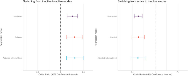 Figure 1
Peer Reviews
No public reviews on file for this paper yet. If you reviewed it on a platform where reviews are public (OpenReview, ICLR, NeurIPS, ICML), you can paste yours below so the community can read it here.
Videos
No videos yet. Explain this paper in a talk, walkthrough, or lecture? Add one.
Taxonomy
TopicsAir Quality and Health Impacts · Urban Transport and Accessibility
Correction **: ** Xiao et al. Int J Behav Nutr Phys Act 21, 89 (2024)
https://doi.org/10.1186/s12966-024-01621-7
Following publication of the original article, the authors identified coding errors in the merging of datasets. Correcting these has resulted in an increased number of participants with complete covariate data. These corrections have had a minimal impact on the main findings; the magnitude of the effects and the primary conclusions remain supported. Page (PDF)IncorrectCorrect1…Among children who took inactive modes at baseline, 42% of children in London and 20% of childrenin Luton switched to active modes. For children taking active modes at baseline, 5% of children in London and 21%of children in Luton switched to inactive modes. Relative to the children in Luton, children in London were more likelyto have switched from inactive to active modes (OR 3.64, 95% CI 1.21–10.92). Children in the intervention group werealso less likely to switch from active to inactive modes (OR 0.11, 0.05–0.24). Moderator analyses showed that childrenliving further from school were more likely to switch from inactive to active modes (OR 6.06,1.87–19.68) comparedto those living closer (OR 1.43, 0.27–7.54)…Among children who took inactive modes at baseline, 42% of children in London and 20% of childrenin Luton switched to active modes. For children taking active modes at baseline, 5% of children in London and 21%of children in Luton switched to inactive modes. Relative to the children in Luton, children in London were more likelyto have switched from inactive to active modes (OR 3.51, 95% CI 1.68–7.31). Children in the intervention group werealso less likely to switch from active to inactive modes (OR 0.22, 0.12–0.41). Moderator analyses showed that childrenliving further from school were more likely to switch from inactive to active modes (OR 5.20; 1.67–15.21) comparedto those living closer (OR 1.54, 0.33–7.21)This value was transformed into a binary variable using a 0.78-km cut-off,This value was transformed into a binary variable using a 0.86-km cut-off,5…distance to school (≤ 0.78 km or > 0.78 km),…distance to school (≤ 0.86 km or > 0.86 km),*A new paragraph needs to be inserted between the 1 st and 2nd paragraph of Data Analysis, as follows:*We encountered convergence issues in the fully adjusted multilevel model for switching from active to inactive modes, likely due to overparameterization. To resolve this, we removed the'parental occupation'variable, as socioeconomic factors were already captured by other covariates (parental employment, crime, IDACI). Sensitivity analyses showed that this exclusion did not significantly affect model fit (likelihood ratio test p = 0.964) and improved AIC and BIC values (Appendix Table 3), indicating a better-fitting, more parsimoniousWe conducted two sensitivity analysesWe conducted additional sensitivity analysesChildren who were not included in the analysis at any time point (reasons for exclusion can be found in Fig. 2) from the London cohort (n = 664) were more likely to be male (48.5% vs. 42.4%), from a minority ethnic background(70.1% vs. 66.3%) and lived closer to school (52.7% vs. 48.0%) compared to children living in London who were included in the analyses (Appendix Table 3). Luton children not included in the analyses (n = 768) were more likely to be older (7.9 vs. 7.7 years) at baseline,less likely to have parents in full-time employment (28.9% vs. 34.9%), more likely to live further from school (63.1%vs. 54.4%) and lived in areas with lower levels of neighbourhood deprivation than children living in Luton whowere included in the analysesChildren who were not included in the analysis at any time point (reasons for exclusion can be found in Fig. 2) from the London cohort (n = 664) were more likely to be male (48.5% vs. 42.4%), from a minority ethnic background (70.1% vs. 66.3%), more likely to have an ‘Other’ occupation (26.8% vs. 18.7%), and lived in areas with higher crime and neighbourhood deprivation compared to children living in London who were included in the analyses (Appendix Table 4). Luton children not included in the analyses (n = 768) were more likely to be older (7.9 vs. 7.7 years) at baseline, less likely to have parents in full-time employment (28.9% vs. 34.9%), more likely to live further from (58.9% vs. 51.7%) and lived in areas with higher levels of crime and neighbourhood deprivation than children living in Luton who were included in the analyses6There may have been evidenceof negative confounding, as the effect size of the fully adjusted model (OR 3.02; 95% CI 1.60–5.70) and the fully adjusted multilevel model (OR 3.64; 95% CI 1.21–10.92) were greater than that of the crude modelThere may have been evidenceof negative confounding, as the effect size of the fully adjusted model (OR 3.47; 95% CI 1.73–7.02) and the fully adjusted multilevel model (OR 3.51; 95% CI 1.68–7.31) were greater than that of the crude modelThe effect sizes of the fully adjusted (OR 0.14, 95% CI 0.08–0.23) and multilevel model (OR 0.11, 0.05–0.24) weresmaller than that of the crude modelThe effect sizes of the fully adjusted (OR 0.23, 95% CI 0.13–0.40) and multilevel model (OR 0.22, 0.12–0.41) were smaller similar to than that of the crude modelAppendix Table 4 and 5Appendix Table 5 and 67Only distance to school statistically significantly moderated the intervention’s effect on switching from inactive to active modes of transport. Specifically, the interaction coefficient was OR 0.24 (95% CI 0.06–0.88), indicating that the intervention’s impact varied depending on the distance to school. Stratified analyses revealed that among children living further from school (> 0.78 km), those in London were significantly more likely to switch to active modes of transport comparedto children in Luton (OR 6.06; 95% CI 1.87–19.68). Conversely, among children living closer to school, there wasno significant evidence of an intervention effect (OR 1.43; 95% CI 0.27–7.54)Distance to school was the only variable that approached statistical significance in moderating the intervention's effect on switching from inactive to active modes of transport. Specifically, the interaction coefficient was OR 0.30 (95% CI 0.08–1.14), indicating that the intervention's impact varied depending on the distance to school. Stratified analyses revealed that among children living further from school (> 0.86 km), those in London were significantly more likely to switch to active modes of transport compared to children in Luton (OR 5.20; 95% CI 1.67–15.21). Conversely, among children living closer to school, there was no significant evidence of an intervention effect (OR 1.54; 95% CI 0.33–7.21)
Moreover, all tables, Fig. 3 and Supplementary Materials need to be updated, as follows:
Table 1. Descriptive baseline characteristics of the study populationCovariateLondon(n = 1000)Luton(n = 982)p-valueAge (mean, SD) Baseline7.9(0.9)7.7(0.9) < 0.001 Follow-up8.9(0.9)8.7(0.7) < 0.001Sex (n, %) Male424(42.4)490(49.9)0.002 Female576(57.6)492(50.1)Ethnicity (n, %) BAME629(66.3)572(59.8) < 0.001 White320(33.7)384(40.2)Employment status (n, %) Full-time279(32.2)317(34.9)0.038 Part-time224(25.9)231(25.4) Unemployed126(14.5)119(13.1) Other237(27.4)241(26.5)Occupational category (n, %) Professional/Managerial368(56.0)310(45.7)0.007 Skilled96(14.6)112(16.5) Unskilled70(10.7)79(11.7) Other123(18.7)177(26.1)Distance to school (n, %) Near (≤ 0.86 km)475**(51.3)351(48.3)0.254 Far (> 0.86 km)451(48.7)375(51.7)Vehicle ownership (n, %) Yes461(54.1)798(89.7) < 0.001 No391(45.9)92(10.3)Crime Quintile (n, %) 1 (highest crime)309**(31.0)302(30.9)** < 0.001 2301****(30.2)328(33.6) 3172****(17.2)237(24.3) 4115****(11.5)89(9.1) 5 (lowest crime)101**(10.1)21(2.1)IDACI Quintile (n, %) 1 (highest level of deprivation)578(57.9)190(19.4)** < 0.001 2269****(27.0)368(37.7) 375****(7.5)282(28.9) 434****(3.4)114(11.7) 5 (lowest level of deprivation)42**(4.2)23(2.4)Sums of the number of participants with each characteristic may equal the total number of participants if data is missingN Number, BAME Black, Asian, and Minority Ethnic, SD Standard deviation, km Kilometre, IDACI Index Deprivation Affecting Children Indexp* value refers to independent samples t-tests for continuous variables or Pearson's χ2 tests for categorical variablesVehicle ownership data was only collected at follow-upTable 2Proportion of children maintaining or switching modes in London and LutonBaselineFollow-upGroupLondonLutonn (%)n (%)ActiveActiveMaintained active modes812 (94%)475 (79%)InactiveSwitched to inactive modes48 (6%)124 (21%)InactiveActiveSwitched to active modes44 (42%)74 (20%)InactiveMaintained inactive modes61 (58%)290 (80%)Table 3. Unadjusted, adjusted, and adjusted multilevel binomial logistic regression models for odds of switching from inactive to active modes and switching from active to inactive modes ‘today’Inactive to ActiveActive to InactivePredictor variableUnadjusted modelAdjusted modelAdjusted multilevel modelUnadjusted modelAdjusted modelAdjusted multilevel modelOROROROROROR(95% CI)(95% CI)(95% CI)(95% CI)(95% CI)(95% CI)Constant0.260.380.330.260.050.05**(0.20—0.33)(0.02—7.98)****(0.01—7.97)(0.21—0.32)(0.00—0.73)(0.00—0.80)London2.833.473.510.230.23****0.22(1.77—4.50)(1.73—7.02)****(1.68—7.31)(0.16—0.32)(0.13—0.40)(0.12—0.41)**Sex (Female)**1.111.110.860.85Ref: Male**(0.63—1.97)(0.63—1.98)(0.55—1.35)(0.54—1.34)Age1.051.061.031.03****(0.71—1.53)(0.71—1.58)(0.76—1.40)(0.75—1.42)**Ethnicity (White)**2.182.190.690.67Ref: BAME(1.18—4.07)(1.17—4.12)(0.42—1.13)(0.40—1.12)**Distance to school (Near ≤ 0.86 km)**3.233.320.270.26Ref: Far (> 0.86 km)(1.75—6.03)(1.75—6.30)(0.16—0.42)(0.16—0.42)**Vehicle ownership (Yes)**0.130.1316.4717.18Ref: No(0.05—0.33)(0.05—0.34)(5.85—69.06)(5.17—57.09)**Employment (Part—time)**1.231.221.301.28Ref: Full—time(0.61—2.45)(0.60—2.47)(0.73—2.30)(0.72—2.28)**Employment (Unemployed)**1.021.021.141.13Ref: Full—time(0.46—2.19)(0.46—2.24)(0.63—2.06)(0.61—2.06)**Employment (Other)**1.561.600.680.67Ref: Full—time(0.57—4.09)(0.59—4.37)(0.30—1.49)(0.30—1.51)**IDACI quintile (linear)**0.760.721.681.72****(0.18—2.67)(0.19—2.77)(0.82—3.33)(0.84—3.51)**Crime quintile (linear)**0.610.641.841.91****(0.15—1.96)(0.18—2.28)(0.85—3.91)(0.86—4.26)Observations4693313311459985985R^2^0.0430.2060.2960.0530.1670.519ICC0.030.03OR Odds ratio, 95% CI 95% Confidence interval, ICC Intraclass correlation coefficientTable 4Adjusted multilevel logistic regression models with interaction termsSwitching from Inactive to Active modesSwitching from Active to Inactive modesModel 1Model 2Model 3Model 4Model 5Model 1Model 2Model 3Model 4**Model 5**Predictor variableOROROROROROROROROROR(95% CI)(95% CI)(95% CI)(95% CI)(95% CI)(95% CI)(95% CI)(95% CI)(95% CI)(95% CI)Constant0.350.110.360.310.240.050.140.050.050.11(0.01—8.37)(0.00—5.99)(0.01—8.88)(0.01—7.26)(0.01—5.90)(0.00—0.81)(0.00—5.58)(0.00—0.78)(0.00—0.79)(0.01—2.22)Site (London) Ref: Luton3.1884.843.15.217.40.220.020.320.240.05(1.18—8.58)(0.10—99.63)(1.34—7.18)(2.23—12.10)(1.56—19.16)(0.10—0.49)(0.00—3.60)(0.15—0.65)(0.12—0.50)(0.00—0.57)Sex (Female) Ref: Male1.051.121.121.061.120.840.850.850.840.85(0.52—2.11)(0.63—2.00)(0.63—1.99)(0.60—1.89)(0.63—2.00)(0.48—1.49)(0.54—1.34)(0.54—1.35)(0.53—1.33)(0.54—1.35)Age1.061.231.061.061.041.030.91.011.031.03(0.71—1.58)(0.74—2.04)(0.71—1.58)(0.71—1.58)(0.70—1.55)(0.75—1.42)(0.58—1.40)(0.74—1.38)(0.75—1.42)(0.75—1.41)Ethnicity (White) Ref: BAME2.22.221.962.22.240.670.680.920.670.68(1.17—4.12)(1.17—4.21)(0.95—4.07)(1.18—4.12)(1.20—4.20)(0.40—1.12)(0.41—1.15)(0.49—1.75)(0.40—1.12)(0.41—1.13)Distance to school (Near ≤ 0.86 km)3.333.423.334.763.270.260.260.260.280.26Ref: Far (> 0.86 km)(1.76—6.33)(1.78—6.55)(1.76—6.33)(2.23—10.13)(1.73—6.18)(0.16—0.42)(0.16—0.42)(0.16—0.42)(0.15—0.50)(0.16—0.43)Vehicle ownership (Yes) Ref: No0.130.120.130.120.2217.1917.0816.9117.337.3(0.05—0.34)(0.05—0.33)(0.05—0.34)(0.05—0.33)(0.07—0.73)(5.17—57.13)(5.14—56.74)(5.09—56.11)(5.21—57.63)(1.57—33.9)London * Sex (Female)1.201.01(0.34—4.21)(0.39—2.60)0.671.33(0.29—1.56)(0.70—2.53)1.510.42(0.38—6.03)(0.14—1.25)0.300.30(0.08—1.14)(0.09—1.00)0.171.24(0.01—2.01)(0.00—5.36)R^2^0.2950.3090.2930.3070.3120.5190.5180.520.6570.647ICC0.030.040.030.010.020.030.030.020.220.21OR Odds ratio, CI Confidence interval, ICC Intraclass correlation coefficient
Fig. 3. Regression model results from unadjusted, adjusted, and adjusted multilevel binomial logistic regression models. Note: Adjusted and adjusted multilevel models are adjusted for by child age, sex, ethnicity, parent’s employment and occupation status, distance to school, household car ownership, and neighbourhood deprivation and crime quintile. In addition, multilevel models include clustering based on the child’s school
The original article has been updated accordingly.
Supplementary Information
Supplementary Material 1.