Forecasting with a Bivariate Hysteretic Time Series Model Incorporating Asymmetric Volatility and Dynamic Correlations
Hong Thi Than

TL;DR
This paper introduces a new financial model that captures dynamic volatility and correlations in financial assets using Bayesian methods and hysteresis.
Contribution
The novelty lies in integrating asymmetric volatility and dynamic correlations within a multivariate hysteretic autoregressive model using Bayesian inference.
Findings
The model effectively captures downside risk dynamics in financial time series.
VaR forecasts from the model pass standard backtesting procedures.
Results on real financial data show improved performance compared to the original model.
Abstract
This study explores asymmetric volatility structures within multivariate hysteretic autoregressive (MHAR) models that incorporate conditional correlations, aiming to flexibly capture the dynamic behavior of global financial assets. The proposed framework integrates regime switching and time-varying delays governed by a hysteresis variable, enabling the model to account for both asymmetric volatility and evolving correlation patterns over time. We adopt a fully Bayesian inference approach using adaptive Markov chain Monte Carlo (MCMC) techniques, allowing for the joint estimation of model parameters, Value-at-Risk (VaR), and Marginal Expected Shortfall (MES). The accuracy of VaR forecasts is assessed through two standard backtesting procedures. Our empirical analysis involves both simulated data and real-world financial datasets to evaluate the model’s effectiveness in capturing downside…
Genes, proteins, chemicals, diseases, species, mutations and cell lines named across the full text — each resolved to its canonical identifier and authoritative record.
Click any figure to enlarge with its caption.
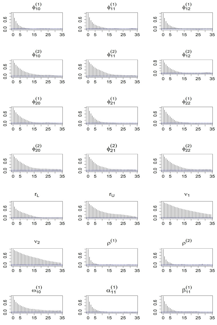 Figure 1
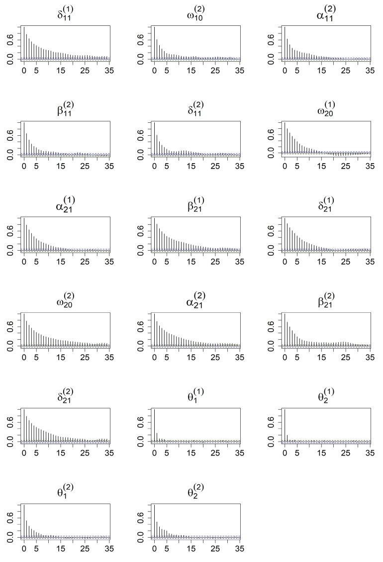 Figure 2
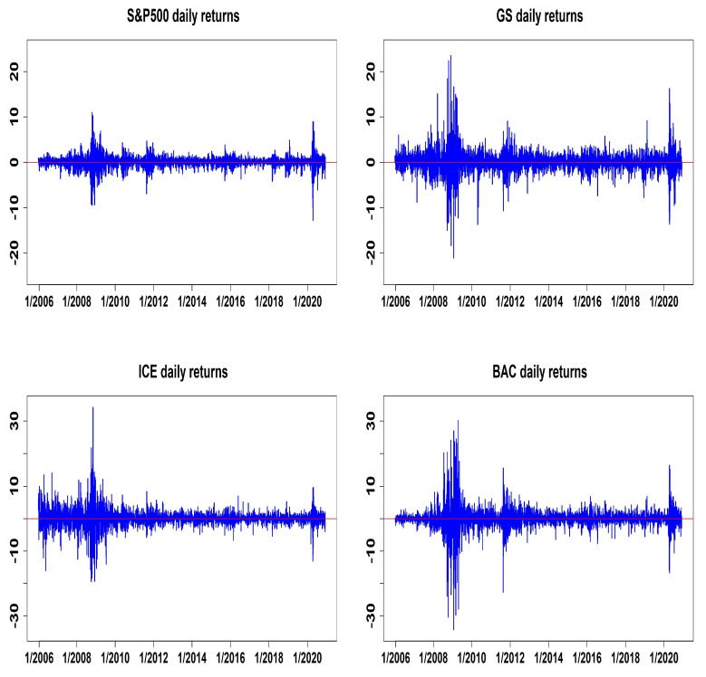 Figure 3
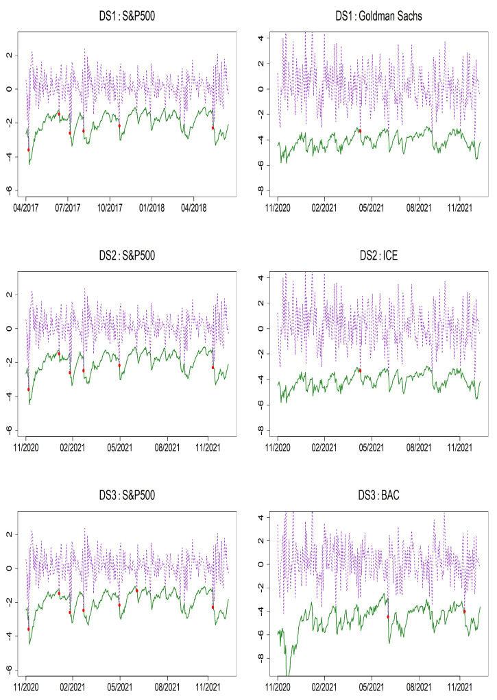 Figure 4
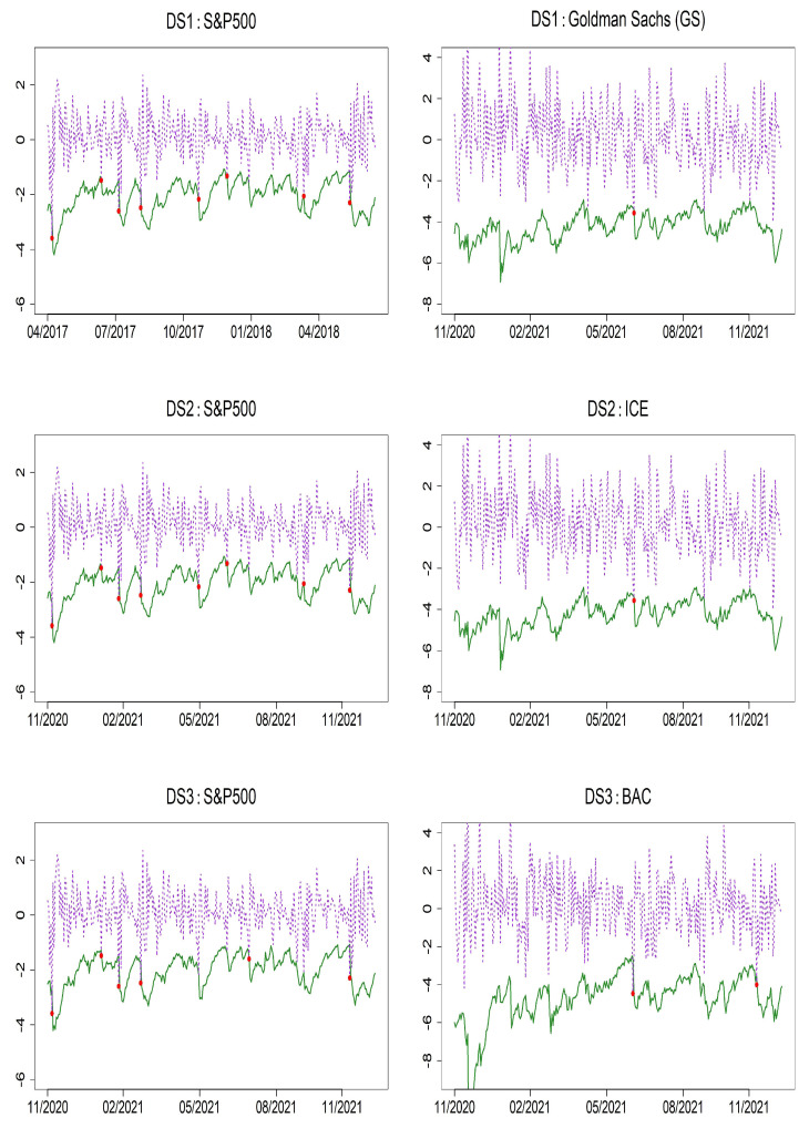 Figure 5
Peer Reviews
No public reviews on file for this paper yet. If you reviewed it on a platform where reviews are public (OpenReview, ICLR, NeurIPS, ICML), you can paste yours below so the community can read it here.
Videos
No videos yet. Explain this paper in a talk, walkthrough, or lecture? Add one.
Taxonomy
TopicsFinancial Risk and Volatility Modeling · Market Dynamics and Volatility · Complex Systems and Time Series Analysis
1. Introduction
Shocks to a time series can cause persistent effects, whereby the influence of disturbances spreads and persists over time. This phenomenon, referred to as the hysteresis effect, reflects a form of path dependence in which system dynamics respond asymmetrically to past shocks. To address issues related to excessive or spurious regime shifts, a range of univariate hysteretic time series models have been developed by the authors of [1,2,3,4,5,6,7]. In financial econometrics, it is well established that asset returns tend to exhibit co-movement. Understanding and forecasting the temporal dependence in the second-order moments of these returns is a key concern in finance. Multivariate models provide a useful framework for capturing complex features such as volatility clustering across multiple assets, time-varying correlations, and joint downside tail risks across industries. These considerations have led researchers to extend univariate volatility models into the multivariate setting. For instance, the authors of [8] introduced the VECH and BEKK models, while the authors of [9] proposed the Dynamic Conditional Correlation (DCC) model, which allows for a time-varying conditional correlation matrix. In contrast, the authors of [10] developed a model that captures correlation dynamics through a weighted average of past correlation matrices, reflecting the persistence of conditional correlations. The authors of [11] developed an asymmetric Dynamic Conditional Correlation (AG-DCC) model to examine the presence of asymmetric responses in conditional volatility and correlation between financial asset returns, particularly allowing for asymmetries in the correlations. A comprehensive discussion on generalized univariate volatility models can be found in [12]. The authors of [13] suggested an extension of [10] using a Bayesian Markov chain Monte Carlo (MCMC) technique to accommodate heavy-tailed distributions. Nonetheless, these models do not consider regime-switching behavior, which is potentially essential for modeling structural shifts and regime-dependent dynamics in financial markets.
In the multivariate context, the authors of [14] proposed the Hysteretic Vector Autoregressive (HVAR) model, which incorporates delayed regime switching based on a hysteresis variable. Specifically, transitions between regimes occur only when this variable exits a predefined hysteresis zone. The authors of [15] introduced a bivariate HAR model incorporating GARCH errors and time-varying correlations. This model integrates features of dynamic correlation, asymmetric effects on correlation and volatility, and heavy-tailed distribution within the multivariate HAR framework previously developed by [14]. However, the asymmetry in [15] is introduced only through the regime-switching behavior of a hysteresis variable within the system. This approach overlooks the leverage effects associated with individual asset returns, which have been emphasized in earlier studies in [11]. In a univariate framework, the authors of [16,17] examined the intricate dynamics between financial returns and volatility, emphasizing the asymmetric effects of shocks. The authors of [16] modified the GARCH model to account for seasonal volatility patterns, differential impacts of positive and negative return innovations, and the influence of nominal interest rates on conditional variance. Similarly, the author of [17] generalized the ARCH framework by modeling the conditional variance as a quadratic function of past innovations, allowing for a nuanced capture of volatility patterns, including asymmetries and leverage effects. Both studies underscore the importance of accommodating asymmetries in volatility modeling to better understand and predict financial market behaviors.
As a result, the volatility specification in [15] leaves room for improvement in modeling asymmetric effects at the level of individual return series. In this paper, we develop an extension of the multivariate hysteretic autoregressive (MHAR) model with GARCH errors and dynamic correlations (see [15]) to accommodate asymmetries in volatility dynamics. Specifically, we incorporate two well-known asymmetric volatility specifications: the GJR-GARCH, as defined in [16], and the QGARCH, proposed in [17]. These extensions result in two model variants, namely, the MHAR–GJR–GARCH and the MHAR–QGARCH models.
To the best of our knowledge, this is the first study to explore asymmetric volatility structures within the MHAR–GARCH framework. By introducing these asymmetric components, the proposed models offer greater flexibility in capturing the heterogeneity and nonlinear behavior commonly observed in financial asset returns. Such flexibility is particularly important in modeling risk dynamics, especially during periods of market turbulence where asymmetries in volatility play a crucial role. Based on the proposed models, we employ an adaptive multivariate t-distribution to account for heavy-tailed errors, and utilize the SMN representation (see [18]) to flexibly model marginal error distributions with varying degrees of freedom, improving the model’s fit to the target time series.
In finance, systemic risk refers to the possibility that problems in one financial institution or a group of them could spread throughout the financial system due to the strong connections between institutions. Such a chain reaction can lead to serious disruptions or even cause the entire market to collapse. Following [19], the Marginal Expected Shortfall (MES) is employed to empirically evaluate the extent to which this risk measure addresses practical concerns related to systemic risk, using a large sample of major U.S. banks. In this study, we consider two widely used risk measures: Value at Risk (VaR) and MES, in which MES plays a more prominent role in capturing tail risk and systemic vulnerability. Additionally, we implement two backtesting procedures to assess the accuracy of out-of-sample VaR forecasts.
A major limitation of the proposed models lies in their increasing complexity, particularly due to the large number of parameters that must be estimated and the challenges involved in modeling nonlinear multivariate structures. As the nonlinearity and asymmetric structures of the proposed models increase, traditional estimation methods become inefficient or impractical. To overcome these difficulties, we adopt a Bayesian framework using Markov chain Monte Carlo (MCMC) techniques, which allows for simultaneous inference of all unknown parameters.
The remainder of this paper is divided into the following sections: The multivariate hysteretic autoregressive model with time-varying correlations and asymmetry structures in volatility is presented in Section 2. Bayesian inference for the model parameters is presented in Section 3. Forecasting VaR and the marginal expected shortfall (MES) are considered in Section 4. Section 5 examines simulation. The empirical study is described in Section 6 and marks are covered in Section 7.
2. Multivariate Hysteretic Autoregressive Model with Asymmetry Structures in Volatility and Time-Varying Correlation
We consider the MHAR–GARCH model, a multivariate hysteretic autoregressive model with GARCH type errors:
and the th element of is formulated as:
where is a vector of k assets at time t, is a regime indicator, is a k-dimensional vector, is a matrix, is a positive-definite matrix with diagonal elements, scalar parameters are satisfied and , and is a sample correlation matrix of shocks from for a pre-specified S. Moreover, is a hysteresis variable. In this study, we investigate two distinct forms of asymmetric volatility within the framework of a multivariate hysteretic autoregressive (MHAR) model. The first approach incorporates the asymmetric volatility structure proposed by [16] into the MHAR–GARCH framework, resulting in the MHAR–GJR–GARCH model. The second approach introduces the quadratic GARCH specification, as developed by the authors of [17], leading to the formulation of the MHAR–QGARCH model. We also derive the volatility dynamics of the MHAR–GJR–GARCH model:
where is a indicator function that returns a value of 1 when the argument is true or 0 otherwise. The volatility of the MHAR - QGARCH model is as follows:
We now consider the basic cases of two models: the bivariate HAR(1)–GJR–GARCH(1,1) model and the bivariate HAR(1)–QGARCH(1,1) model. We assume that innovations in Equation (1) follow the modified bivariate Student’s-t distribution (see [15]). In this case, we apply the scale SMN representation (see [18]) to the adapted bivariate Student’s-t distribution, , and we choose . Then, the bivariate HAR(1)–GJR–GARCH(1,1) model is described as follows:
where the th element of is described in (2) and the conditional volitilities as follows:
where is a indicator function that returns a value of 1 when the argument is true or 0 otherwise. The positivity and stationarity conditions for volatility are given as follows:
The bivariate HAR(1)–QGARCH(1,1) model modifies the conditional volatilities as follows:
where the positivity and stationarity conditions for volatility are given as follows:
and we specify the unconditional correlation matrix :
3. Bayesian Inference
To estimate the unknown parameters of the proposed models in a Bayesian framework, for example, we create groups of the unknown parameters: (i) ; (ii) ; (iii) ; (iv) ; (v) , ; (vi) and (vii) d. We define as a vector of all the unknown parameters of the proposed model. Following that, the bivariate HAR(1)–GJR–GARCH(1,1) and bivariate HAR(1)–QGARCH(1,1) models’ conditional likelihood functions are given by:
where .
We set up prior distributions for the unknown parameters. Assume that ; for the threshold parameter , where and are the pth and th percentiles of the observed time series, respectively, for Furthermore, where is the th percentile and for is a selected number that ensures and at least of observations are in the range . For the degrees of freedom, we assume the scale mixture variables and , and . For the lag d, we choose the discrete uniform prior with maximum delay . In terms of the volatility parameters, follows a uniform distribution such that is proportional to or , where and are the sets that satisfy (4) and (5), respectively.
The conditional posterior distribution for each group is proportional to the conditional likelihood function multiplied by the prior density for that group, as shown below:
where is each parameter group, is its prior density, and is the vector of all parameters, except . The conditional posterior distribution of the delay lag d follows a multinomial distribution with a probability:
In this study, with the exception of the lag parameter d, the conditional posterior distributions of the remaining parameter groups exhibit non-standard forms. To make a statistical inference, we employ an adaptive Markov chain Monte Carlo (MCMC) method for selected parameter groups, complemented by a random walk Metropolis algorithm. Specifically, we assume that the innovation term in Equation (3) follows a Gaussian distribution, which serves as the kernel for sampling . For the parameter groups and , where , an adaptive MCMC approach is utilized to draw samples, whereas the remaining parameters are updated using the random walk Metropolis algorithm. The detailed procedures of the adaptive Metropolis–Hastings MCMC algorithm are thoroughly presented by the authors of [1,15], where the authors provide a comprehensive framework for its implementation and application. Following the guidelines of [1], we further adjust the scale matrix to attain ideal acceptance rates of to .
In a Bayesian framework, we need to set up the initial values for each parameter group. For the autoregressive coefficient parameters, ; for the degrees of freedom ; ; ; ; and ; thresholds and are established at the 33rd and 67th percentiles, respectively; and we set to make certain of having enough observations in each regime for a valid inference. For the remainder of the analysis, we specify .
4. Forecasting the Marginal Expected Shortfall and Value at Risk
The Value-at-Risk (VaR) and Marginal Expected Shortfall (MES) are now considered systemic risk assessments for financial risk management. The authors of [19] define MES as a financial firm’s marginal contribution to the financial system’s expected shortfall. The authors of [20] define MES at the alpha level for a financial institution at time t given as follows:
where is the VaR of at the -level such that . Here, stands for the stock return of a financial institution, whereas stands for the market return.
To produce , we estimate one-step-ahead quantiles and volatilities for from the investigated model described in (3) with forecast origin . We obtain quantiles from the posterior predictive distribution, which is:
Suppose that are the rth MCMC drawn from the posterior density after the burn-in sample. Thus, we can sample from the marginal predictive distribution, , by sampling the following conditional distribution:
where and are a conditional mean and the covariance of at the rth iteration. To assess the correctness of a VaR performance, we calculate the violation rate (VRate). The accuracy of a VaR performance is verified by recording the failure rate; that is, the violation rate:
where is the out-of-sample period size and is the return at time t. We use two tests to assess the validity of the VaR forecasts: the conditional coverage (CC) test created by [21] and the unconditional coverage (UC) test created by [22]. The CC test is conducted to investigate the null hypothesis that the violations are independently distributed, whereas the UC test is applied to determine whether the percentage of violations is equivalent to the VaR significance level.
5. Simulation Study
In order to access the effectiveness of the Bayesian approach, we run two simulations of the suggested models in this section. Model 1 is the bivariate HAR(1)–GJR–GARCH(1,1) model and Model 2 is the bivariate HAR(1)–QGARCH(1,1) model. Model 1 is given by:
Model 2 is described as follows:
Models 1 and 2 are created utilizing the actual values shown in Table 1 and Table 2. For each time series, we set up the sample size n = 2000. We carry out N = 30,000 MCMC iterations and discard the first M = 10,000 burn-in iterates. For the hyper–parameters, we choose the initial values for all parameters of the investigated model to be , , , , , , and .
The results for the parameter estimates of the simulation study are shown in Table 1 and Table 2. The tables present the posterior means, medians, standard deviations, and credible ranges for Models 1–2 over the 200 replications. We observe that the credible interval contains the corresponding true value for each parameter. The posterior means and medians in each case are fairly close to the true parameter values. The posterior modes of lag d are demonstrated, and it can be explained that the posterior mode of d provides a reliable estimate of the delay parameter because the posterior probability for is nearly equal to one. To check the convergence of MCMC, we examine the ACF plots of all coefficients. For compactness, we present only the autocorrelation function (ACF) plots based on Model 2, omitting the ACF plots of Model 1 to conserve space. Figure 1 and Figure 2 provide additional evidence supporting the convergence of the MCMC algorithm. Based on these diagnostic checks, we conclude that the proposed models are well suited for implementation within the Bayesian framework.
6. Emperical Study
The empirical analysis in this study is based on the daily closing prices of four major financial indices: the S&P500, Bank of America (BAC), Intercontinental Exchange (ICE), and Goldman Sachs (GS). The data span from 4 January 2006, to 30 December 2021, encompassing a total of 4026 trading days. These data were retrieved from Yahoo Finance, a widely recognized source for historical market data. To construct the return series, we compute the continuously compounded returns (log-returns) using the formula , where denotes the asset’s closing price at time t.
Table 3 defines three target datasets: DS1 {S&P500, GS}, DS2 {S&P500, ICE}, and DS3 {S&P500, BAC}. It also presents the descriptive statistics of the corresponding return series, along with the results of two multivariate normality tests: Mardia’s test and the Henze–Zirkler test (see [23,24]). The return distributions are clearly skewed and have high kurtosis, in particular, showing strong positive skewness. Due to the noticeable asymmetry and the presence of heavy tails in the return data, we recommend using asymmetric models with fat-tailed multivariate error distributions instead of models that assume multivariate normal errors. Figure 3 presents the time series plot of daily returns for the selected financial assets. As shown, the sample period spans several significant market events, notably the Global Financial Crisis, which officially began on 15 September 2008, following the bankruptcy of Lehman Brothers. For the purpose of estimation and out-of-sample evaluation, the dataset is divided into two distinct sub-periods. The first segment, consisting of 3726 daily observations, is used to estimate the model parameters. The remaining 300 observations are reserved for out-of-sample forecasting and performance assessment.
This section’s hyper-parameters correspond to those in the simulation study. Table 4, Table 5, Table 6 and Table 7 present a summary of the Bayesian estimates for three datasets for the BHAR(1)–GJR–GARCH(1,1) and the BHAR(1)–QGARCH(1,1) models. The significant value of in Table 4 and Table 6 indicates that the performance of the previous day’s return of Goldman Sachs stock has a considerable negative impact on the S&P 500’s returns in the lower regimes. We can see that the parameter estimates for , , , and are identical in both fitted models when we look at datasets DS2 and DS3 in Table 5 and Table 7. To assess the validity of the proposed models, we further employ the Geweke convergence diagnostic (see [25]). The p-values reported in Table 8 and Table 9 suggest that the MCMC chains generated from the models have converged. As there is no statistical evidence of non-convergence, we conclude that the proposed models are appropriately specified and reliable for inference.
To evaluate the accuracy of the models using Value-at-Risk (VaR), we present VaR forecasts along with the results of VaR backtesting at the 1% and 5% significance levels. Specifically, Table 10 and Table 11 report the p-values of the Unconditional Coverage (UC) and Conditional Coverage (CC) tests for the two proposed models: bivariate HAR(1)–GJR–GARCH(1,1) and HAR(1)–QGARCH(1,1) as well as the benchmark bivariate HAR(1)–GARCH(1,1) model. When evaluating DS1, DS2, and DS3 across the three models, the violation rates (VRate) for the S&P 500 tend to be significantly higher than the nominal 1% level, suggesting a slight underestimation of tail risk. In contrast, the VRates for Bank of America (BAC), Intercontinental Exchange (ICE), and Goldman Sachs (GS) indicate a tendency toward risk overestimation. Nevertheless, the backtesting results show that all three models perform adequately as risk models. At the 5% significance level, both the proposed models and the benchmark BHAR(1)–GARCH(1,1) model yield UC and CC test p-values above 5%, indicating no statistical evidence of model misspecification. These findings confirm that the proposed models deliver reliable and independent risk forecasts. Figure 4 and Figure 5 display the VaR forecasts based on the bivariate HAR(1)–GJR–GARCH(1,1) and HAR(1)–QGARCH(1,1) models, which clearly show that the models are capable of identifying volatility spikes in returns, despite infrequent violations of the forecast bounds.
To understand how well the proposed models can capture the expected shortfall movement, we present the backtesting measures of the MES forecasts proposed by the authors of [26] in Table 12. The model with the smallest values in the boxes is the best. These findings indicate that the proposed models are the best.
7. Conclusions
This paper investigates the MHAR–GJR–GARCH and MHAR–QGARCH models by incorporating asymmetric volatility dynamics, conditional correlations, and a hysteresis variable to control regime switching and dynamic delays. Bayesian inference is employed for efficient estimation of the model parameters. A comparative analysis of backtesting results for the VaR and MES forecasts is conducted. We also include the benchmark model MHAR–GARCH with adapted multivariate Student’s-t errors and compare backtesting measures of the Value-at-Risk (VaR) and Marginal Expected Shortfall (MES) forecasts. The backtesting measures indicate that, in general, the proposed models demonstrate reliable capabilities in capturing tail risk behavior and delivering accurate risk predictions. Notably, the proposed models deliver significantly improved performance over the original MHAR–GARCH errors model, particularly in capturing asymmetric tail risks and providing more accurate risk forecasts. An interesting direction for future research involves incorporating entropy-based measures, such as those discussed in [27,28], as complementary indicators of volatility and structural regime shifts. As entropy captures informational complexity and system disorder, it may enhance regime detection when combined with hysteresis-based models.
The reference list from the paper itself. Each links out to its DOI / PubMed record.
- 1Chen C.W.S. So M.K.P. On a threshold heteroscedastic model Int. J. Forecast.200622738910.1016/j.ijforecast.2005.08.001 · doi ↗
- 2Chen C.W.S. Truong B.C. On double hysteretic heteroskedastic model J. Stat. Comput. Simul.2016862684270510.1080/00949655.2015.1123262 · doi ↗
- 3Li G.D. Guan B. Li W.K. Yu P.L.H. Hysteretic autoregressive time series models Biometrika 201510271772310.1093/biomet/asv 017 · doi ↗
- 4Lo P.H. Li W.K. Yu P.L.H. Li G.D. On buffered threshold GARCH models Stat. Sin.2016261555156710.5705/ss.2014.098t · doi ↗
- 5Truong B.C. Chen C.W. Sriboonchitta S. Hysteretic Poisson INGARCH model for integer-valued time series Stat. Model.20171740142210.1177/1471082 X 17703855 · doi ↗
- 6Zhu K. Yu P.L.H. Li W.K. Testing for the buffered autoregressive processes Stat. Sin.20142497198410.5705/ss.2012.311 · doi ↗
- 7Zhu K. Li W.K. Yu P.L.H. Buffered autoregressive models with conditional heteroskedasticity: An application to exchange rates J. Bus. Econ. Stat.20173552854210.1080/07350015.2015.1123634 · doi ↗
- 8Bollerslev T. On the correlation structure for the generalized autoregressive conditional heteroskedastic process J. Time Ser. Anal.1988912113110.1111/j.1467-9892.1988.tb 00459.x · doi ↗