Computing the distance between unbalanced distributions: the flat metric
Henri Schmidt, Christian Düll

TL;DR
This paper introduces a new way to compute distances between unbalanced data distributions using a neural network-based method.
Contribution
The paper provides an implementation of the flat metric for unbalanced distributions using a neural network approach.
Findings
The flat metric generalizes the Wasserstein distance to unbalanced distributions.
A neural network is used to compute optimal test functions for distance calculation.
The method was validated with experiments and simulated data.
Abstract
We provide an implementation to compute the flat metric in any dimension. The flat metric, also called dual bounded Lipschitz distance, generalizes the well-known Wasserstein distance \documentclass[12pt]{minimal} \usepackage{amsmath} \usepackage{wasysym} \usepackage{amsfonts} \usepackage{amssymb} \usepackage{amsbsy} \usepackage{mathrsfs} \usepackage{upgreek} \setlength{\oddsidemargin}{-69pt} \begin{document}\end{document}W1 to the case that the distributions are of unequal total mass. Thus, our implementation adapts very well to mass differences and uses them to distinguish between different distributions. This is of particular interest for unbalanced optimal transport tasks and for the analysis of data distributions where the sample size is important or normalization is not possible. The core of the method is based on a neural network to…
Click any figure to enlarge with its caption.
 Figure 10
 Figure 11
 Figure 12
 Figure 13
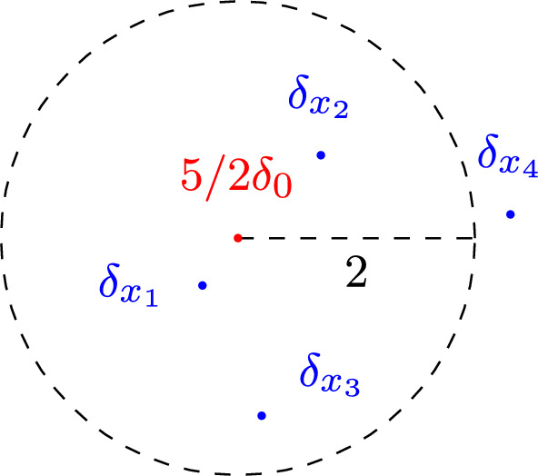 Figure 14
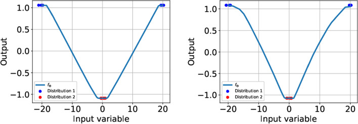 Figure 1
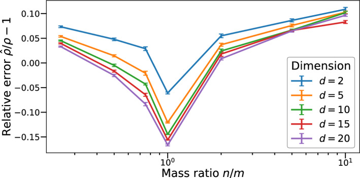 Figure 2
 Figure 3
 Figure 4
 Figure 5
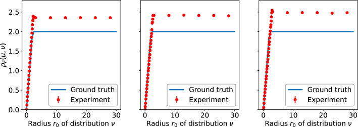 Figure 6
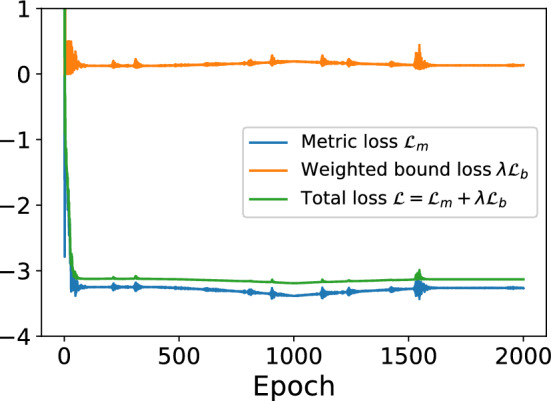 Figure 7
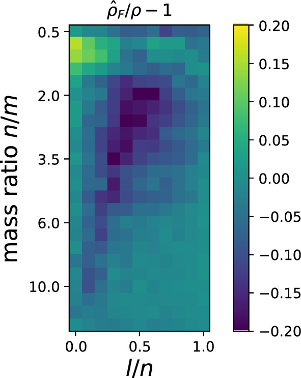 Figure 8
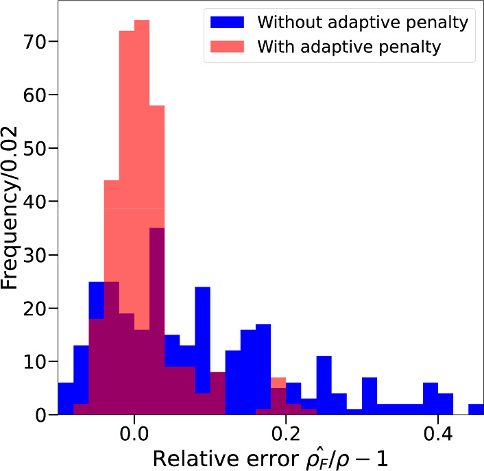 Figure 9
- —http://dx.doi.org/10.13039/501100001659Deutsche Forschungsgemeinschaft
- —http://dx.doi.org/10.13039/100019180HORIZON EUROPE European Research Council
- —Ruprecht-Karls-Universität Heidelberg (1026)
Peer Reviews
No public reviews on file for this paper yet. If you reviewed it on a platform where reviews are public (OpenReview, ICLR, NeurIPS, ICML), you can paste yours below so the community can read it here.
Videos
No videos yet. Explain this paper in a talk, walkthrough, or lecture? Add one.
Taxonomy
TopicsGenerative Adversarial Networks and Image Synthesis · Markov Chains and Monte Carlo Methods · Medical Image Segmentation Techniques
Introduction
This paper is devoted to a method for computing the flat metric between two nonnegative Radon measures of potentially unequal total mass, realized by a neural network. Special focus lies on an implementation which allows for comparability of pairwise computed distances from independently trained networks. To this end, we extend the Wasserstein framework developed by Anil et al. (2019) to the unbalanced case.
The paper is structured as follows: In the remainder of the introduction we define the flat metric and give a short overview on unbalanced optimal transport. As will be evident from the definition, test functions for the flat metric have to be Lipschitz continuous so that we modify a neural network approach for the Wasserstein metric (Anil et al., 2019) to our setting. Section 2 is devoted to the architecture of the neural network as well as the subsequent adjustment of the output via experiments with ground truth to compensate for systematic errors. In Sect. 3 we provide experimental validation of our method and residual analysis, whereas the conclusion is given in Sect. 4. Additional information on the calibration of the method, the adaptive penalty as well as on the hyperparameters and experimental details can be found in the Appendix. Furthermore, it contains a novel analytical distance result for Dirac measures in the flat metric.
Background
We will consider measures with different masses, so that we work in \documentclass[12pt]{minimal} \usepackage{amsmath} \usepackage{wasysym} \usepackage{amsfonts} \usepackage{amssymb} \usepackage{amsbsy} \usepackage{mathrsfs} \usepackage{upgreek} \setlength{\oddsidemargin}{-69pt} \begin{document}$$\mathcal {M}^+(\mathbb {R}^d)$$\end{document} , i.e. the cone of nonnegative, bounded real-valued Borel measures on \documentclass[12pt]{minimal} \usepackage{amsmath} \usepackage{wasysym} \usepackage{amsfonts} \usepackage{amssymb} \usepackage{amsbsy} \usepackage{mathrsfs} \usepackage{upgreek} \setlength{\oddsidemargin}{-69pt} \begin{document}$$\mathbb {R}^d$$\end{document} . We equip \documentclass[12pt]{minimal} \usepackage{amsmath} \usepackage{wasysym} \usepackage{amsfonts} \usepackage{amssymb} \usepackage{amsbsy} \usepackage{mathrsfs} \usepackage{upgreek} \setlength{\oddsidemargin}{-69pt} \begin{document}$$\mathcal {M}^+(\mathbb {R}^d)$$\end{document} with the flat metric (or dual bounded Lipschitz distance, Fortet-Mourier distance) defined by
\documentclass[12pt]{minimal} \usepackage{amsmath} \usepackage{wasysym} \usepackage{amsfonts} \usepackage{amssymb} \usepackage{amsbsy} \usepackage{mathrsfs} \usepackage{upgreek} \setlength{\oddsidemargin}{-69pt} \begin{document}$$\begin{aligned} \rho _F(\mu ,\nu )= \sup _{\Vert f\Vert _{BL} \le 1}\int _{\mathbb {R}^d} f \,\textrm{d}(\mu -\nu ). \end{aligned}$$\end{document}The class of test functions is given by the bounded Lipschitz functions endowed with the norm \documentclass[12pt]{minimal} \usepackage{amsmath} \usepackage{wasysym} \usepackage{amsfonts} \usepackage{amssymb} \usepackage{amsbsy} \usepackage{mathrsfs} \usepackage{upgreek} \setlength{\oddsidemargin}{-69pt} \begin{document}$$\Vert f\Vert _{BL} = \max \left( \Vert f\Vert _{\infty }, \, |f|_{\textbf{Lip}}\right) $$\end{document} , where \documentclass[12pt]{minimal} \usepackage{amsmath} \usepackage{wasysym} \usepackage{amsfonts} \usepackage{amssymb} \usepackage{amsbsy} \usepackage{mathrsfs} \usepackage{upgreek} \setlength{\oddsidemargin}{-69pt} \begin{document}$$\Vert f\Vert _{\infty }=\underset{x\in \mathbb {R}^d}{\sup }\,|f(x)|$$\end{document} and \documentclass[12pt]{minimal} \usepackage{amsmath} \usepackage{wasysym} \usepackage{amsfonts} \usepackage{amssymb} \usepackage{amsbsy} \usepackage{mathrsfs} \usepackage{upgreek} \setlength{\oddsidemargin}{-69pt} \begin{document}$$|f|_{\textbf{Lip}}=\underset{ x\ne y}{\sup }\, \frac{|f(x)-f(y)|}{|x-y|}$$\end{document} . Note that formulation (1.1) resembles the Kantorovich-Rubinstein duality of the Wasserstein distance \documentclass[12pt]{minimal} \usepackage{amsmath} \usepackage{wasysym} \usepackage{amsfonts} \usepackage{amssymb} \usepackage{amsbsy} \usepackage{mathrsfs} \usepackage{upgreek} \setlength{\oddsidemargin}{-69pt} \begin{document}$$W_1$$\end{document} , i.e.
\documentclass[12pt]{minimal} \usepackage{amsmath} \usepackage{wasysym} \usepackage{amsfonts} \usepackage{amssymb} \usepackage{amsbsy} \usepackage{mathrsfs} \usepackage{upgreek} \setlength{\oddsidemargin}{-69pt} \begin{document}$$\begin{aligned} W_1(\mu ,\nu )=\sup _{|f|_{\textbf{Lip}}\le 1} \int _{\mathbb {R}^d}f \,\textrm{d}(\mu -\nu ). \end{aligned}$$\end{document}Coming from optimal transport (OT) theory (Cuturi, 2013; Villani, 2003, 2009), the Wasserstein metrics define distances between probability measures which take into account the geometry of the underlying state space. Consequently, distances with respect to the Wasserstein metrics are more informative than methods based on divergences (Grauman & Darrell, 2004; Ling & Okada, 2007; Peyré et al., 2012; Villani, 2003, 2009). Note that the Wasserstein distances scale with the total mass of the measures \documentclass[12pt]{minimal} \usepackage{amsmath} \usepackage{wasysym} \usepackage{amsfonts} \usepackage{amssymb} \usepackage{amsbsy} \usepackage{mathrsfs} \usepackage{upgreek} \setlength{\oddsidemargin}{-69pt} \begin{document}$$\mu ,\nu $$\end{document} and are thus not necessarily restricted to probability measures. However, by construction the distances are only applicable in conservative problems, i.e. only if \documentclass[12pt]{minimal} \usepackage{amsmath} \usepackage{wasysym} \usepackage{amsfonts} \usepackage{amssymb} \usepackage{amsbsy} \usepackage{mathrsfs} \usepackage{upgreek} \setlength{\oddsidemargin}{-69pt} \begin{document}$$\mu (\mathbb {R}^d)=\nu (\mathbb {R}^d)$$\end{document} , as otherwise no optimal transport plan exists, see e.g. (Ulikowska, 2013, Remark 1.18).
In most applications the distributions are normalized to probability measures so that any initial mass difference between the distributions is usually irrelevant. However, if the data distributions cannot be normalized, e.g. as the mass differences of the distributions are actually meaningful since the underlying process is not conservative, then the data has to be artificially renormalized for OT to be applicable or the OT approach has to be discarded. This problem naturally appears in population dynamics with growth and death processes, see for example (Schiebinger et al., 2019; Zhang et al., 2021) where the authors employed the (entropically regularized) Wasserstein metric to compute distances between single cell gene distributions of cell samples in order to infer developmental trajectories. To compensate for the inherent cell growth over time, the authors had to introduce an additional model function which eliminates the impact of increasing cell numbers. However, these problems also occur in other areas, such as in imaging or seismic analysis where the signal intensities fluctuate or even oscillate around 0, so that data can not be normalized (Lee et al., 2020; Li et al., 2022).
Thus, in recent years numerous approaches appeared to tackle these unbalanced OT tasks, see (Chizat et al., 2018; Peyré & Cuturi, 2019) for an overview of several approaches on unbalanced optimal transport. In contrast to classical OT, there is no mass restriction with unbalanced OT so that mass between distributions can not only be transported, but also created or destroyed. Among the most important applications are generative adversarial networks (Balaji et al., 2020; Yang & Uhler, 2019), domain adaptation (Fatras et al., 2021; Tran et al., 2023), color transfer (Sonthalia & Gilbert, 2020) and outlier detection (Mukherjee et al., 2021; Balaji et al., 2020). Since the unbalanced OT schemes can choose to ignore parts of the distribution due to mass deletion, they are quite robust to outliers (Mukherjee et al., 2021; Balaji et al., 2020).
However, the aim of this work is not to find an optimal (unbalanced) transportation plan, but a reliable way to compare measures with each other via a reasonable metric which simplifies interpretability of the distances. From the purely theoretical side, the obvious candidate would be given by the well-established total variation (TV) norm
\documentclass[12pt]{minimal} \usepackage{amsmath} \usepackage{wasysym} \usepackage{amsfonts} \usepackage{amssymb} \usepackage{amsbsy} \usepackage{mathrsfs} \usepackage{upgreek} \setlength{\oddsidemargin}{-69pt} \begin{document}$$\begin{aligned} \Vert \mu \Vert _{TV}:=\mu ^+(\mathbb {R}^d)+\mu ^-(\mathbb {R}^d), \end{aligned}$$\end{document}where \documentclass[12pt]{minimal} \usepackage{amsmath} \usepackage{wasysym} \usepackage{amsfonts} \usepackage{amssymb} \usepackage{amsbsy} \usepackage{mathrsfs} \usepackage{upgreek} \setlength{\oddsidemargin}{-69pt} \begin{document}$$\mu ^+,\mu ^-\in \mathcal {M}^+(\mathbb {R}^d)$$\end{document} are the measures arising from Jordan decomposition theorem (Folland, 1984, Theorem 3.4). However, as \documentclass[12pt]{minimal} \usepackage{amsmath} \usepackage{wasysym} \usepackage{amsfonts} \usepackage{amssymb} \usepackage{amsbsy} \usepackage{mathrsfs} \usepackage{upgreek} \setlength{\oddsidemargin}{-69pt} \begin{document}$$\Vert \cdot \Vert _{TV}$$\end{document} completely ignores the underlying geometry, this norm is is not suited for data which is obvious when computing the TV distance between two Dirac measures of the form
\documentclass[12pt]{minimal} \usepackage{amsmath} \usepackage{wasysym} \usepackage{amsfonts} \usepackage{amssymb} \usepackage{amsbsy} \usepackage{mathrsfs} \usepackage{upgreek} \setlength{\oddsidemargin}{-69pt} \begin{document}$$\delta _a(x)=\left\{ \begin{array}{cc}1,& x=a\\ 0,& \text {else}\end{array}.\right.$$\end{document}One readily computes the distance to be
\documentclass[12pt]{minimal} \usepackage{amsmath} \usepackage{wasysym} \usepackage{amsfonts} \usepackage{amssymb} \usepackage{amsbsy} \usepackage{mathrsfs} \usepackage{upgreek} \setlength{\oddsidemargin}{-69pt} \begin{document}$$\begin{aligned} \Vert \delta _a-\delta _b\Vert _{TV}=\delta _a(\mathbb {R}^d)+\delta _b(\mathbb {R}^d)=2 \qquad \forall a,b\in \mathbb {R}^d, a\ne b, \end{aligned}$$\end{document}independent from the distance of the support points a, b. So instead we choose the flat metric defined by (1.1). Apart from convenient analytical properties, providing completeness and separability for the measure space \documentclass[12pt]{minimal} \usepackage{amsmath} \usepackage{wasysym} \usepackage{amsfonts} \usepackage{amssymb} \usepackage{amsbsy} \usepackage{mathrsfs} \usepackage{upgreek} \setlength{\oddsidemargin}{-69pt} \begin{document}$$\mathcal {M}^+(\mathbb {R}^d)$$\end{document} (Gwiazda et al., 2018), the flat metric acts as a suitable generalization of the 1-Wasserstein distance \documentclass[12pt]{minimal} \usepackage{amsmath} \usepackage{wasysym} \usepackage{amsfonts} \usepackage{amssymb} \usepackage{amsbsy} \usepackage{mathrsfs} \usepackage{upgreek} \setlength{\oddsidemargin}{-69pt} \begin{document}$$W_1$$\end{document} to unbalanced tasks, and is as such also geometrically faithful, at least locally (see A2). This is illustrated by the following alternative characterization due to Piccoli and Rossi (Piccoli & Rossi, 2014, Theorem 13):
\documentclass[12pt]{minimal} \usepackage{amsmath} \usepackage{wasysym} \usepackage{amsfonts} \usepackage{amssymb} \usepackage{amsbsy} \usepackage{mathrsfs} \usepackage{upgreek} \setlength{\oddsidemargin}{-69pt} \begin{document}$$\begin{aligned} \rho _F(\mu ,\nu )= \inf _{\begin{array}{c} \tilde{\mu }\le \mu ,\,\tilde{\nu }\le \nu \\ \Vert \tilde{\mu }\Vert _{TV}=\Vert \tilde{\nu }\Vert _{TV} \end{array}}\Vert \mu -\tilde{\mu }\Vert _{TV}+\Vert \nu -\tilde{\nu }\Vert _{TV}+W_1(\tilde{\mu },\tilde{\nu }). \end{aligned}$$\end{document}The decomposition (1.3) of \documentclass[12pt]{minimal} \usepackage{amsmath} \usepackage{wasysym} \usepackage{amsfonts} \usepackage{amssymb} \usepackage{amsbsy} \usepackage{mathrsfs} \usepackage{upgreek} \setlength{\oddsidemargin}{-69pt} \begin{document}$$\rho _F$$\end{document} into terms with TV norm and the term with Wasserstein distance admits the typical interpretation of mass transport versus mass deletion: any share \documentclass[12pt]{minimal} \usepackage{amsmath} \usepackage{wasysym} \usepackage{amsfonts} \usepackage{amssymb} \usepackage{amsbsy} \usepackage{mathrsfs} \usepackage{upgreek} \setlength{\oddsidemargin}{-69pt} \begin{document}$$\delta \mu $$\end{document} of the mass of \documentclass[12pt]{minimal} \usepackage{amsmath} \usepackage{wasysym} \usepackage{amsfonts} \usepackage{amssymb} \usepackage{amsbsy} \usepackage{mathrsfs} \usepackage{upgreek} \setlength{\oddsidemargin}{-69pt} \begin{document}$$\mu $$\end{document} can either be transported from \documentclass[12pt]{minimal} \usepackage{amsmath} \usepackage{wasysym} \usepackage{amsfonts} \usepackage{amssymb} \usepackage{amsbsy} \usepackage{mathrsfs} \usepackage{upgreek} \setlength{\oddsidemargin}{-69pt} \begin{document}$$\mu $$\end{document} to \documentclass[12pt]{minimal} \usepackage{amsmath} \usepackage{wasysym} \usepackage{amsfonts} \usepackage{amssymb} \usepackage{amsbsy} \usepackage{mathrsfs} \usepackage{upgreek} \setlength{\oddsidemargin}{-69pt} \begin{document}$$\nu $$\end{document} at cost \documentclass[12pt]{minimal} \usepackage{amsmath} \usepackage{wasysym} \usepackage{amsfonts} \usepackage{amssymb} \usepackage{amsbsy} \usepackage{mathrsfs} \usepackage{upgreek} \setlength{\oddsidemargin}{-69pt} \begin{document}$$W_1(\delta \mu ,\delta \nu )$$\end{document} or removed/generated at cost \documentclass[12pt]{minimal} \usepackage{amsmath} \usepackage{wasysym} \usepackage{amsfonts} \usepackage{amssymb} \usepackage{amsbsy} \usepackage{mathrsfs} \usepackage{upgreek} \setlength{\oddsidemargin}{-69pt} \begin{document}$$\Vert \delta \mu \Vert _{TV}$$\end{document} . As such, the minimal "sub-measures" \documentclass[12pt]{minimal} \usepackage{amsmath} \usepackage{wasysym} \usepackage{amsfonts} \usepackage{amssymb} \usepackage{amsbsy} \usepackage{mathrsfs} \usepackage{upgreek} \setlength{\oddsidemargin}{-69pt} \begin{document}$$\tilde{\mu },\tilde{\nu }$$\end{document} achieve an optimal compromise between the strategy of mass transportation and of removal/generation. With regard to the implementation of the flat metric, we expect both regimes to display different associated errors that have to be accounted for individually.
The flat metric has been used in Lellmann et al. (2014) for inverse problems in imaging and recently to establish well-posedness theory for structured population models in measures on separable and complete metric spaces (Düll et al., 2022).
In view of (1.3) we note that the approach introduced in Mukherjee et al. (2021) tends to come closest to our setting as they also introduced a TV norm constraint instead of the typical Kullback–Leibler divergence to introduce an unbalanced optimization problem. Nevertheless, we choose to compute \documentclass[12pt]{minimal} \usepackage{amsmath} \usepackage{wasysym} \usepackage{amsfonts} \usepackage{amssymb} \usepackage{amsbsy} \usepackage{mathrsfs} \usepackage{upgreek} \setlength{\oddsidemargin}{-69pt} \begin{document}$$\rho _F$$\end{document} via (1.1) and not (1.3).
At this point, we would like to remark that the goal of our implementation is not to achieve superior computational performance over already established methods, but merely to provide another perspective. Although our method can in principal handle distributions of arbitrary dimension, the treatment of high-dimensional distributions generally requires more data points, so that our proposed method becomes computationally expensive for dimensions \documentclass[12pt]{minimal} \usepackage{amsmath} \usepackage{wasysym} \usepackage{amsfonts} \usepackage{amssymb} \usepackage{amsbsy} \usepackage{mathrsfs} \usepackage{upgreek} \setlength{\oddsidemargin}{-69pt} \begin{document}$$d=20$$\end{document} and higher. At this point we refer to a recent paper (Lakshmanan & Pichler, 2024) which applies nonequispaced fast Fourier transform to speed up the computations for radial kernels in unbalanced optimal transport tasks, so that high-dimensional data sets can be handled efficiently.
Methods
Given two measures \documentclass[12pt]{minimal} \usepackage{amsmath} \usepackage{wasysym} \usepackage{amsfonts} \usepackage{amssymb} \usepackage{amsbsy} \usepackage{mathrsfs} \usepackage{upgreek} \setlength{\oddsidemargin}{-69pt} \begin{document}$$\mu ,\nu \in \mathcal {M}^+(\mathbb {R}^d)$$\end{document} , explicitly computing their flat distance via (1.1) is highly nontrivial as finding a closed analytical expressions for the flat metric proves to be complicated even for Dirac measures, see Proposition 1. So instead we trained a neural network of two fully connected hidden layers with 64 neurons each and the Adam optimizer (Kingma & Ba, 2015) to approximate \documentclass[12pt]{minimal} \usepackage{amsmath} \usepackage{wasysym} \usepackage{amsfonts} \usepackage{amssymb} \usepackage{amsbsy} \usepackage{mathrsfs} \usepackage{upgreek} \setlength{\oddsidemargin}{-69pt} \begin{document}$$\rho _F(\mu ,\nu )$$\end{document} using (1.1). Note that we deliberately chose a shallow network architecture as it provides sufficiently good results whereas moving to larger networks results in instabilities or even failures during training due to limited training data. In view of the Universal Approximation Theorem proven in Anil et al. (2019), a suitable choice of architectural constraints allows the whole space \documentclass[12pt]{minimal} \usepackage{amsmath} \usepackage{wasysym} \usepackage{amsfonts} \usepackage{amssymb} \usepackage{amsbsy} \usepackage{mathrsfs} \usepackage{upgreek} \setlength{\oddsidemargin}{-69pt} \begin{document}$$BL(\mathbb {R}^d)$$\end{document} to be accessed via the network, so that we can expect meaningful results.
We make the ansatz \documentclass[12pt]{minimal} \usepackage{amsmath} \usepackage{wasysym} \usepackage{amsfonts} \usepackage{amssymb} \usepackage{amsbsy} \usepackage{mathrsfs} \usepackage{upgreek} \setlength{\oddsidemargin}{-69pt} \begin{document}$$f=f_\Theta $$\end{document} and model the optimal bounded Lipschitz test function by a multi-layer perceptron. To ensure that \documentclass[12pt]{minimal} \usepackage{amsmath} \usepackage{wasysym} \usepackage{amsfonts} \usepackage{amssymb} \usepackage{amsbsy} \usepackage{mathrsfs} \usepackage{upgreek} \setlength{\oddsidemargin}{-69pt} \begin{document}$$f_\Theta $$\end{document} is indeed admissible to the problem, i.e. that it is a bounded Lipschitz function with \documentclass[12pt]{minimal} \usepackage{amsmath} \usepackage{wasysym} \usepackage{amsfonts} \usepackage{amssymb} \usepackage{amsbsy} \usepackage{mathrsfs} \usepackage{upgreek} \setlength{\oddsidemargin}{-69pt} \begin{document}$$\Vert \cdot \Vert _{BL}$$\end{document} norm bounded by 1, we use a mixed approach of regularization and architectural constraints. In particular, we adopt the architectural approach introduced in Anil et al. (2019) to guarantee Lipschitz continuity whereas we use regularizational constraints to account for the optimization problem (1.1) and to enforce boundedness of \documentclass[12pt]{minimal} \usepackage{amsmath} \usepackage{wasysym} \usepackage{amsfonts} \usepackage{amssymb} \usepackage{amsbsy} \usepackage{mathrsfs} \usepackage{upgreek} \setlength{\oddsidemargin}{-69pt} \begin{document}$$f_{\Theta }$$\end{document} .
Architectural constraints
In Anil et al. (2019) the authors Anil, Lucas and Grosse constructed a neural network to calculate the Wasserstein distance \documentclass[12pt]{minimal} \usepackage{amsmath} \usepackage{wasysym} \usepackage{amsfonts} \usepackage{amssymb} \usepackage{amsbsy} \usepackage{mathrsfs} \usepackage{upgreek} \setlength{\oddsidemargin}{-69pt} \begin{document}$$W_1$$\end{document} via its Kantorovich-Rubinstein duality (1.2). Their approach is based on the fact that Lipschitz continuity is closed under compositions, so that it is sufficient to control the Lipschitz constant of each individual layer and activation function. In order to compute \documentclass[12pt]{minimal} \usepackage{amsmath} \usepackage{wasysym} \usepackage{amsfonts} \usepackage{amssymb} \usepackage{amsbsy} \usepackage{mathrsfs} \usepackage{upgreek} \setlength{\oddsidemargin}{-69pt} \begin{document}$$W_1$$\end{document} Anil, Lucas and Grosse proposed to normalize each layer \documentclass[12pt]{minimal} \usepackage{amsmath} \usepackage{wasysym} \usepackage{amsfonts} \usepackage{amssymb} \usepackage{amsbsy} \usepackage{mathrsfs} \usepackage{upgreek} \setlength{\oddsidemargin}{-69pt} \begin{document}$$A_i$$\end{document} and to use the 1-Lipschitz shuffling operator GroupSort (Chernodub & Nowicki, 2017) as activation function. This way the authors are able to construct a universal Lipschitz approximator. Hence, adopting the network architecture will yield Lipschitz continuity of \documentclass[12pt]{minimal} \usepackage{amsmath} \usepackage{wasysym} \usepackage{amsfonts} \usepackage{amssymb} \usepackage{amsbsy} \usepackage{mathrsfs} \usepackage{upgreek} \setlength{\oddsidemargin}{-69pt} \begin{document}$$f_{\Theta }$$\end{document} . We shortly summarize the most important concepts of the paper.
In Anil et al. (2019) the authors apply Björck orthonormalization (Björck & Bowie, 1971) during each forward pass which ensures that the linear transformation induced by layer \documentclass[12pt]{minimal} \usepackage{amsmath} \usepackage{wasysym} \usepackage{amsfonts} \usepackage{amssymb} \usepackage{amsbsy} \usepackage{mathrsfs} \usepackage{upgreek} \setlength{\oddsidemargin}{-69pt} \begin{document}$$A_i$$\end{document} is in fact isometric, thus strictly enforcing \documentclass[12pt]{minimal} \usepackage{amsmath} \usepackage{wasysym} \usepackage{amsfonts} \usepackage{amssymb} \usepackage{amsbsy} \usepackage{mathrsfs} \usepackage{upgreek} \setlength{\oddsidemargin}{-69pt} \begin{document}$$|A_i|_{\textbf{Lip}} = 1$$\end{document} . While this is convenient for the computation of \documentclass[12pt]{minimal} \usepackage{amsmath} \usepackage{wasysym} \usepackage{amsfonts} \usepackage{amssymb} \usepackage{amsbsy} \usepackage{mathrsfs} \usepackage{upgreek} \setlength{\oddsidemargin}{-69pt} \begin{document}$$W_1$$\end{document} as the test function f will always be 1-Lipschitz theoretically, in our setting a Björck orthonormalization is too restrictive as in practice the optimal \documentclass[12pt]{minimal} \usepackage{amsmath} \usepackage{wasysym} \usepackage{amsfonts} \usepackage{amssymb} \usepackage{amsbsy} \usepackage{mathrsfs} \usepackage{upgreek} \setlength{\oddsidemargin}{-69pt} \begin{document}$$f_\Theta $$\end{document} of the flat distance often has a smaller Lipschitz constant \documentclass[12pt]{minimal} \usepackage{amsmath} \usepackage{wasysym} \usepackage{amsfonts} \usepackage{amssymb} \usepackage{amsbsy} \usepackage{mathrsfs} \usepackage{upgreek} \setlength{\oddsidemargin}{-69pt} \begin{document}$$|f_\Theta |_{\textbf{Lip}}$$\end{document} . Thus, in our implementation we necessarily have to switch to spectral normalization \documentclass[12pt]{minimal} \usepackage{amsmath} \usepackage{wasysym} \usepackage{amsfonts} \usepackage{amssymb} \usepackage{amsbsy} \usepackage{mathrsfs} \usepackage{upgreek} \setlength{\oddsidemargin}{-69pt} \begin{document}$$\Vert A_i\Vert _2=1$$\end{document} instead which ensures that the largest singular value is 1 but there may be other eigenspaces with smaller absolute singular values. In particular, we do not require \documentclass[12pt]{minimal} \usepackage{amsmath} \usepackage{wasysym} \usepackage{amsfonts} \usepackage{amssymb} \usepackage{amsbsy} \usepackage{mathrsfs} \usepackage{upgreek} \setlength{\oddsidemargin}{-69pt} \begin{document}$$A_i$$\end{document} to be 1-Lipschitz in every direction but just enforce \documentclass[12pt]{minimal} \usepackage{amsmath} \usepackage{wasysym} \usepackage{amsfonts} \usepackage{amssymb} \usepackage{amsbsy} \usepackage{mathrsfs} \usepackage{upgreek} \setlength{\oddsidemargin}{-69pt} \begin{document}$$|A_i|_{\textbf{Lip}} \le 1$$\end{document} . As the spectral normalization—in contrast to Björk orthonomalization—is not gradient norm preserving, our choice potentially leads to diminishing gradient norms of the network during backpropagation and thus to slower convergence of the network, see (Anil et al., 2019, B.2).
Nevertheless, the Björck and the spectral normalization yield similar results for a simple toy problem presented in Fig. 1. In particular, the Björck approach is also able to produce gradients with norm less than one between probability measures \documentclass[12pt]{minimal} \usepackage{amsmath} \usepackage{wasysym} \usepackage{amsfonts} \usepackage{amssymb} \usepackage{amsbsy} \usepackage{mathrsfs} \usepackage{upgreek} \setlength{\oddsidemargin}{-69pt} \begin{document}$$\mu , \nu $$\end{document} . This is rather surprising as in the Wasserstein case (i.e. without a bound constraint in the loss) \documentclass[12pt]{minimal} \usepackage{amsmath} \usepackage{wasysym} \usepackage{amsfonts} \usepackage{amssymb} \usepackage{amsbsy} \usepackage{mathrsfs} \usepackage{upgreek} \setlength{\oddsidemargin}{-69pt} \begin{document}$$f_\Theta $$\end{document} should indeed attain \documentclass[12pt]{minimal} \usepackage{amsmath} \usepackage{wasysym} \usepackage{amsfonts} \usepackage{amssymb} \usepackage{amsbsy} \usepackage{mathrsfs} \usepackage{upgreek} \setlength{\oddsidemargin}{-69pt} \begin{document}$$|\nabla f_\Theta |=1$$\end{document} due to the linear 1-Lipschitz layers, see also (Gulrajani et al., 2017, Corollary 1). We assume that the bound constraint (2.3) interferes with the normalization, such that the linear layers are in fact not completely orthonormal.Fig. 1A simple 1D experiment showing the similarities between spectral normalization (left) and Björck orthonormalization (right). We considered two Gaussian mixture models \documentclass[12pt]{minimal} \usepackage{amsmath} \usepackage{wasysym} \usepackage{amsfonts} \usepackage{amssymb} \usepackage{amsbsy} \usepackage{mathrsfs} \usepackage{upgreek} \setlength{\oddsidemargin}{-69pt} \begin{document}$$\mu =\frac{128}{2}(\mathcal {N}(-20, 0.5)+\mathcal {N}(20, 0.5))$$\end{document} (blue) and \documentclass[12pt]{minimal} \usepackage{amsmath} \usepackage{wasysym} \usepackage{amsfonts} \usepackage{amssymb} \usepackage{amsbsy} \usepackage{mathrsfs} \usepackage{upgreek} \setlength{\oddsidemargin}{-69pt} \begin{document}$$\nu =128\mathcal {N}(0, 0.5)$$\end{document} (red). In both cases the resulting \documentclass[12pt]{minimal} \usepackage{amsmath} \usepackage{wasysym} \usepackage{amsfonts} \usepackage{amssymb} \usepackage{amsbsy} \usepackage{mathrsfs} \usepackage{upgreek} \setlength{\oddsidemargin}{-69pt} \begin{document}$$f_\Theta $$\end{document} was plotted. Each time \documentclass[12pt]{minimal} \usepackage{amsmath} \usepackage{wasysym} \usepackage{amsfonts} \usepackage{amssymb} \usepackage{amsbsy} \usepackage{mathrsfs} \usepackage{upgreek} \setlength{\oddsidemargin}{-69pt} \begin{document}$$f_{\theta }$$\end{document} is bounded and \documentclass[12pt]{minimal} \usepackage{amsmath} \usepackage{wasysym} \usepackage{amsfonts} \usepackage{amssymb} \usepackage{amsbsy} \usepackage{mathrsfs} \usepackage{upgreek} \setlength{\oddsidemargin}{-69pt} \begin{document}$$|f_{\Theta }|_{\textbf{Lip}}\ll 1$$\end{document} (Color figure online)
The activation function GroupSort is a nonlinear, 1-Lipschitz operator which generalizes ReLU (Anil et al., 2019). It separates the pre-activations into groups and within each group permutes the input yielding an isometry. Typically, we will use two pre-activations per group, though higher values can be chosen too. In contrast to ReLU, GroupSort prevents gradient norm attenuation which would lead to \documentclass[12pt]{minimal} \usepackage{amsmath} \usepackage{wasysym} \usepackage{amsfonts} \usepackage{amssymb} \usepackage{amsbsy} \usepackage{mathrsfs} \usepackage{upgreek} \setlength{\oddsidemargin}{-69pt} \begin{document}$$|f_\Theta |_{\textbf{Lip}} \ll 1$$\end{document} for deep networks. It often arises as a ReLU unit will map half of its input space to zero, thereby effacing all of the previous layers’ gradients in this region. In fact, it can be shown that a weight-constraint and norm-preserving neural network with ReLU activations is in fact linear (Anil et al., 2019). Due to the lack of computational complexity, such a network is undesirable and thus the challenge is to construct a neural network which is 1-Lipschitz and simultaneously maintains enough expressive power to be a universal approximator. Both, in the work by Anil et al. (2019) and our work GroupSort has proven to work well while preserving enough expressive power to be a universal approximator.
Note that in view of Tsuzuku et al. (2018) a Lipschitz constrained network provides provable adversarial robustness, i.e. the change in output under small adversarial perturbations is bounded.
Regularization constraints
Our loss term has to account for both the optimization problem of the flat metric and the boundedness constraint for \documentclass[12pt]{minimal} \usepackage{amsmath} \usepackage{wasysym} \usepackage{amsfonts} \usepackage{amssymb} \usepackage{amsbsy} \usepackage{mathrsfs} \usepackage{upgreek} \setlength{\oddsidemargin}{-69pt} \begin{document}$$f_{\Theta }$$\end{document} , so that the total loss term \documentclass[12pt]{minimal} \usepackage{amsmath} \usepackage{wasysym} \usepackage{amsfonts} \usepackage{amssymb} \usepackage{amsbsy} \usepackage{mathrsfs} \usepackage{upgreek} \setlength{\oddsidemargin}{-69pt} \begin{document}$$\mathcal {L}$$\end{document} consists of two parts
\documentclass[12pt]{minimal} \usepackage{amsmath} \usepackage{wasysym} \usepackage{amsfonts} \usepackage{amssymb} \usepackage{amsbsy} \usepackage{mathrsfs} \usepackage{upgreek} \setlength{\oddsidemargin}{-69pt} \begin{document}$$\begin{aligned} \mathcal {L} := \mathcal {L}_m + \lambda \mathcal {L}_b. \end{aligned}$$\end{document}The metric loss term \documentclass[12pt]{minimal} \usepackage{amsmath} \usepackage{wasysym} \usepackage{amsfonts} \usepackage{amssymb} \usepackage{amsbsy} \usepackage{mathrsfs} \usepackage{upgreek} \setlength{\oddsidemargin}{-69pt} \begin{document}$$\mathcal {L}_m$$\end{document} corresponds to minimizing the negative of (1.1) and is given by
\documentclass[12pt]{minimal} \usepackage{amsmath} \usepackage{wasysym} \usepackage{amsfonts} \usepackage{amssymb} \usepackage{amsbsy} \usepackage{mathrsfs} \usepackage{upgreek} \setlength{\oddsidemargin}{-69pt} \begin{document}$$\begin{aligned} \mathcal {L}_m:=- \int _{\mathbb {R}^d}f_{\Theta }(x)\,\textrm{d}\mu (x)+\int _{\mathbb {R}^d}f_{\Theta }(x)\,\textrm{d}\nu (x). \end{aligned}$$\end{document}Note that after training \documentclass[12pt]{minimal} \usepackage{amsmath} \usepackage{wasysym} \usepackage{amsfonts} \usepackage{amssymb} \usepackage{amsbsy} \usepackage{mathrsfs} \usepackage{upgreek} \setlength{\oddsidemargin}{-69pt} \begin{document}$$\mathcal {L}_m$$\end{document} is our estimator for (the negative value of) the flat distance \documentclass[12pt]{minimal} \usepackage{amsmath} \usepackage{wasysym} \usepackage{amsfonts} \usepackage{amssymb} \usepackage{amsbsy} \usepackage{mathrsfs} \usepackage{upgreek} \setlength{\oddsidemargin}{-69pt} \begin{document}$$\rho _F(\mu ,\nu )$$\end{document} .
The additional penalty term to bound \documentclass[12pt]{minimal} \usepackage{amsmath} \usepackage{wasysym} \usepackage{amsfonts} \usepackage{amssymb} \usepackage{amsbsy} \usepackage{mathrsfs} \usepackage{upgreek} \setlength{\oddsidemargin}{-69pt} \begin{document}$$f_{\Theta }$$\end{document} is provided by the bound loss term
\documentclass[12pt]{minimal} \usepackage{amsmath} \usepackage{wasysym} \usepackage{amsfonts} \usepackage{amssymb} \usepackage{amsbsy} \usepackage{mathrsfs} \usepackage{upgreek} \setlength{\oddsidemargin}{-69pt} \begin{document}$$\begin{aligned} \mathcal {L}_{b}&\left( \frac{1}{\Vert \mu \Vert _{TV}}\langle h_\mu , h_\mu \rangle + \frac{1}{\Vert \nu \Vert _{TV}} \langle h_\nu , h_\nu \rangle \right) , \end{aligned}$$\end{document}where \documentclass[12pt]{minimal} \usepackage{amsmath} \usepackage{wasysym} \usepackage{amsfonts} \usepackage{amssymb} \usepackage{amsbsy} \usepackage{mathrsfs} \usepackage{upgreek} \setlength{\oddsidemargin}{-69pt} \begin{document}$$h_\kappa :==\max _{x\sim \kappa }(|f_\Theta (x)| - M, 0)$$\end{document} and the parameter M refers to the upper bound for \documentclass[12pt]{minimal} \usepackage{amsmath} \usepackage{wasysym} \usepackage{amsfonts} \usepackage{amssymb} \usepackage{amsbsy} \usepackage{mathrsfs} \usepackage{upgreek} \setlength{\oddsidemargin}{-69pt} \begin{document}$$\Vert f_\Theta \Vert _\infty $$\end{document} which in our formulation is given by \documentclass[12pt]{minimal} \usepackage{amsmath} \usepackage{wasysym} \usepackage{amsfonts} \usepackage{amssymb} \usepackage{amsbsy} \usepackage{mathrsfs} \usepackage{upgreek} \setlength{\oddsidemargin}{-69pt} \begin{document}$$M=1$$\end{document} . By choosing this approach over simply considering the maximal value \documentclass[12pt]{minimal} \usepackage{amsmath} \usepackage{wasysym} \usepackage{amsfonts} \usepackage{amssymb} \usepackage{amsbsy} \usepackage{mathrsfs} \usepackage{upgreek} \setlength{\oddsidemargin}{-69pt} \begin{document}$$\Vert f_\Theta \Vert _\infty $$\end{document} , we reduce the effect of outliers in the data, thus simplifying training. The auxiliary functions \documentclass[12pt]{minimal} \usepackage{amsmath} \usepackage{wasysym} \usepackage{amsfonts} \usepackage{amssymb} \usepackage{amsbsy} \usepackage{mathrsfs} \usepackage{upgreek} \setlength{\oddsidemargin}{-69pt} \begin{document}$$h_\kappa $$\end{document} encode in which areas \documentclass[12pt]{minimal} \usepackage{amsmath} \usepackage{wasysym} \usepackage{amsfonts} \usepackage{amssymb} \usepackage{amsbsy} \usepackage{mathrsfs} \usepackage{upgreek} \setlength{\oddsidemargin}{-69pt} \begin{document}$$f_\Theta $$\end{document} deviates from its target bound evaluated each on the input given by \documentclass[12pt]{minimal} \usepackage{amsmath} \usepackage{wasysym} \usepackage{amsfonts} \usepackage{amssymb} \usepackage{amsbsy} \usepackage{mathrsfs} \usepackage{upgreek} \setlength{\oddsidemargin}{-69pt} \begin{document}$$\kappa =\mu $$\end{document} and \documentclass[12pt]{minimal} \usepackage{amsmath} \usepackage{wasysym} \usepackage{amsfonts} \usepackage{amssymb} \usepackage{amsbsy} \usepackage{mathrsfs} \usepackage{upgreek} \setlength{\oddsidemargin}{-69pt} \begin{document}$$\kappa =\nu $$\end{document} respectively. If such a deflection \documentclass[12pt]{minimal} \usepackage{amsmath} \usepackage{wasysym} \usepackage{amsfonts} \usepackage{amssymb} \usepackage{amsbsy} \usepackage{mathrsfs} \usepackage{upgreek} \setlength{\oddsidemargin}{-69pt} \begin{document}$$|f_\Theta | > 1=M$$\end{document} occurs, the corresponding \documentclass[12pt]{minimal} \usepackage{amsmath} \usepackage{wasysym} \usepackage{amsfonts} \usepackage{amssymb} \usepackage{amsbsy} \usepackage{mathrsfs} \usepackage{upgreek} \setlength{\oddsidemargin}{-69pt} \begin{document}$$h_\kappa $$\end{document} will have non-vanishing values in the appropriate domain and \documentclass[12pt]{minimal} \usepackage{amsmath} \usepackage{wasysym} \usepackage{amsfonts} \usepackage{amssymb} \usepackage{amsbsy} \usepackage{mathrsfs} \usepackage{upgreek} \setlength{\oddsidemargin}{-69pt} \begin{document}$$h_\kappa $$\end{document} serves as a penalty. The penalties are then accumulated over the whole space by the inner product \documentclass[12pt]{minimal} \usepackage{amsmath} \usepackage{wasysym} \usepackage{amsfonts} \usepackage{amssymb} \usepackage{amsbsy} \usepackage{mathrsfs} \usepackage{upgreek} \setlength{\oddsidemargin}{-69pt} \begin{document}$$\langle \cdot ,\cdot \rangle $$\end{document} , which thus measures how much \documentclass[12pt]{minimal} \usepackage{amsmath} \usepackage{wasysym} \usepackage{amsfonts} \usepackage{amssymb} \usepackage{amsbsy} \usepackage{mathrsfs} \usepackage{upgreek} \setlength{\oddsidemargin}{-69pt} \begin{document}$$f_\Theta $$\end{document} violates the bound when evaluated with respect to \documentclass[12pt]{minimal} \usepackage{amsmath} \usepackage{wasysym} \usepackage{amsfonts} \usepackage{amssymb} \usepackage{amsbsy} \usepackage{mathrsfs} \usepackage{upgreek} \setlength{\oddsidemargin}{-69pt} \begin{document}$$\mu $$\end{document} and \documentclass[12pt]{minimal} \usepackage{amsmath} \usepackage{wasysym} \usepackage{amsfonts} \usepackage{amssymb} \usepackage{amsbsy} \usepackage{mathrsfs} \usepackage{upgreek} \setlength{\oddsidemargin}{-69pt} \begin{document}$$\nu $$\end{document} respectively. As the loss term should not favour measures with large total masses, we normalize each contribution by its respective total variation ensuring that the penalty terms remain invariant under scaling of the total mass. This will be useful as our implementation only considers discrete measures where the total variation is simply the number of support points so that it doesn’t matter whether the same empiric distribution is given by 100 or 1000 data points.
The two penalty contributions with respect to \documentclass[12pt]{minimal} \usepackage{amsmath} \usepackage{wasysym} \usepackage{amsfonts} \usepackage{amssymb} \usepackage{amsbsy} \usepackage{mathrsfs} \usepackage{upgreek} \setlength{\oddsidemargin}{-69pt} \begin{document}$$\mu $$\end{document} and \documentclass[12pt]{minimal} \usepackage{amsmath} \usepackage{wasysym} \usepackage{amsfonts} \usepackage{amssymb} \usepackage{amsbsy} \usepackage{mathrsfs} \usepackage{upgreek} \setlength{\oddsidemargin}{-69pt} \begin{document}$$\nu $$\end{document} are then combined to give the overall penalty \documentclass[12pt]{minimal} \usepackage{amsmath} \usepackage{wasysym} \usepackage{amsfonts} \usepackage{amssymb} \usepackage{amsbsy} \usepackage{mathrsfs} \usepackage{upgreek} \setlength{\oddsidemargin}{-69pt} \begin{document}$$\mathcal {L}_b$$\end{document} incurred by violating bound M. In practice, enforcing the ideal bound of a vanishing \documentclass[12pt]{minimal} \usepackage{amsmath} \usepackage{wasysym} \usepackage{amsfonts} \usepackage{amssymb} \usepackage{amsbsy} \usepackage{mathrsfs} \usepackage{upgreek} \setlength{\oddsidemargin}{-69pt} \begin{document}$$\mathcal {L}_b$$\end{document} is not possible in general and hence we strive for small values of the loss. Due to the inner product, penalty contributions enter quadratically in \documentclass[12pt]{minimal} \usepackage{amsmath} \usepackage{wasysym} \usepackage{amsfonts} \usepackage{amssymb} \usepackage{amsbsy} \usepackage{mathrsfs} \usepackage{upgreek} \setlength{\oddsidemargin}{-69pt} \begin{document}$$\mathcal {L}_b$$\end{document} punishing larger deviations from M more severely than smaller ones.
As 1-Lipschitz continuity of \documentclass[12pt]{minimal} \usepackage{amsmath} \usepackage{wasysym} \usepackage{amsfonts} \usepackage{amssymb} \usepackage{amsbsy} \usepackage{mathrsfs} \usepackage{upgreek} \setlength{\oddsidemargin}{-69pt} \begin{document}$$f_{\Theta }$$\end{document} will be guaranteed by the network architecture, the combined loss \documentclass[12pt]{minimal} \usepackage{amsmath} \usepackage{wasysym} \usepackage{amsfonts} \usepackage{amssymb} \usepackage{amsbsy} \usepackage{mathrsfs} \usepackage{upgreek} \setlength{\oddsidemargin}{-69pt} \begin{document}$$\mathcal {L}$$\end{document} then accounts for both rendering \documentclass[12pt]{minimal} \usepackage{amsmath} \usepackage{wasysym} \usepackage{amsfonts} \usepackage{amssymb} \usepackage{amsbsy} \usepackage{mathrsfs} \usepackage{upgreek} \setlength{\oddsidemargin}{-69pt} \begin{document}$$f_\Theta $$\end{document} admissible to the optimization problem (1.1) as well as finding the optimal value of the flat metric. Such an approach of having one loss term for the problem and one for the admissibility is commonly employed, e.g in the implementation of Wasserstein gradient-penalty adversarial networks (Gulrajani et al., 2017). We remark that in (2.1) both contributions act antagonistically as a decrease in \documentclass[12pt]{minimal} \usepackage{amsmath} \usepackage{wasysym} \usepackage{amsfonts} \usepackage{amssymb} \usepackage{amsbsy} \usepackage{mathrsfs} \usepackage{upgreek} \setlength{\oddsidemargin}{-69pt} \begin{document}$$\mathcal {L}_m$$\end{document} often leads to an increase in \documentclass[12pt]{minimal} \usepackage{amsmath} \usepackage{wasysym} \usepackage{amsfonts} \usepackage{amssymb} \usepackage{amsbsy} \usepackage{mathrsfs} \usepackage{upgreek} \setlength{\oddsidemargin}{-69pt} \begin{document}$$\mathcal {L}_b$$\end{document} , see Fig. 7, where the individual loss terms are monitored during training.
Note that the two loss contributions \documentclass[12pt]{minimal} \usepackage{amsmath} \usepackage{wasysym} \usepackage{amsfonts} \usepackage{amssymb} \usepackage{amsbsy} \usepackage{mathrsfs} \usepackage{upgreek} \setlength{\oddsidemargin}{-69pt} \begin{document}$$\mathcal {L}_m$$\end{document} and \documentclass[12pt]{minimal} \usepackage{amsmath} \usepackage{wasysym} \usepackage{amsfonts} \usepackage{amssymb} \usepackage{amsbsy} \usepackage{mathrsfs} \usepackage{upgreek} \setlength{\oddsidemargin}{-69pt} \begin{document}$$\mathcal {L}_b$$\end{document} of \documentclass[12pt]{minimal} \usepackage{amsmath} \usepackage{wasysym} \usepackage{amsfonts} \usepackage{amssymb} \usepackage{amsbsy} \usepackage{mathrsfs} \usepackage{upgreek} \setlength{\oddsidemargin}{-69pt} \begin{document}$$\mathcal {L}$$\end{document} in (2.1) are effectively balanced by an enforcing parameter \documentclass[12pt]{minimal} \usepackage{amsmath} \usepackage{wasysym} \usepackage{amsfonts} \usepackage{amssymb} \usepackage{amsbsy} \usepackage{mathrsfs} \usepackage{upgreek} \setlength{\oddsidemargin}{-69pt} \begin{document}$$\lambda =\lambda (t)$$\end{document} which depends on the fraction of elapsed training t. Specifically, \documentclass[12pt]{minimal} \usepackage{amsmath} \usepackage{wasysym} \usepackage{amsfonts} \usepackage{amssymb} \usepackage{amsbsy} \usepackage{mathrsfs} \usepackage{upgreek} \setlength{\oddsidemargin}{-69pt} \begin{document}$$\lambda $$\end{document} is chosen adaptively so that each freshly trained network is approximately bound by the same constant \documentclass[12pt]{minimal} \usepackage{amsmath} \usepackage{wasysym} \usepackage{amsfonts} \usepackage{amssymb} \usepackage{amsbsy} \usepackage{mathrsfs} \usepackage{upgreek} \setlength{\oddsidemargin}{-69pt} \begin{document}$$\Vert f_\Theta \Vert _\infty \le M$$\end{document} while simultaneously having comparable relative loss contributions of \documentclass[12pt]{minimal} \usepackage{amsmath} \usepackage{wasysym} \usepackage{amsfonts} \usepackage{amssymb} \usepackage{amsbsy} \usepackage{mathrsfs} \usepackage{upgreek} \setlength{\oddsidemargin}{-69pt} \begin{document}$$\mathcal {L}_m$$\end{document} and \documentclass[12pt]{minimal} \usepackage{amsmath} \usepackage{wasysym} \usepackage{amsfonts} \usepackage{amssymb} \usepackage{amsbsy} \usepackage{mathrsfs} \usepackage{upgreek} \setlength{\oddsidemargin}{-69pt} \begin{document}$$\mathcal {L}_b$$\end{document} regardless of the input distributions. This is particularly important for our setting as we want to establish pairwise comparisons of neural networks which have been trained independently and/or on different data sets. This regularly occurs when computing pairwise distances between subdistributions so that the output of the network should be ordinal. Without proper balancing the resulting \documentclass[12pt]{minimal} \usepackage{amsmath} \usepackage{wasysym} \usepackage{amsfonts} \usepackage{amssymb} \usepackage{amsbsy} \usepackage{mathrsfs} \usepackage{upgreek} \setlength{\oddsidemargin}{-69pt} \begin{document}$$f_{\Theta }$$\end{document} will adhere more or less strict to the \documentclass[12pt]{minimal} \usepackage{amsmath} \usepackage{wasysym} \usepackage{amsfonts} \usepackage{amssymb} \usepackage{amsbsy} \usepackage{mathrsfs} \usepackage{upgreek} \setlength{\oddsidemargin}{-69pt} \begin{document}$$\Vert \cdot \Vert _{\infty }$$\end{document} bound depending on the currently dominating loss term leading to biased results. Notably, different networks would solve different optimization problems (1.1) yielding their actual outcomes to be incomparable to each other. Furthermore, each network requires a different optimal \documentclass[12pt]{minimal} \usepackage{amsmath} \usepackage{wasysym} \usepackage{amsfonts} \usepackage{amssymb} \usepackage{amsbsy} \usepackage{mathrsfs} \usepackage{upgreek} \setlength{\oddsidemargin}{-69pt} \begin{document}$$\lambda $$\end{document} , so that we can not simply fix one sufficiently large value for \documentclass[12pt]{minimal} \usepackage{amsmath} \usepackage{wasysym} \usepackage{amsfonts} \usepackage{amssymb} \usepackage{amsbsy} \usepackage{mathrsfs} \usepackage{upgreek} \setlength{\oddsidemargin}{-69pt} \begin{document}$$\lambda $$\end{document} for the bound constraint \documentclass[12pt]{minimal} \usepackage{amsmath} \usepackage{wasysym} \usepackage{amsfonts} \usepackage{amssymb} \usepackage{amsbsy} \usepackage{mathrsfs} \usepackage{upgreek} \setlength{\oddsidemargin}{-69pt} \begin{document}$$\Vert f_\Theta \Vert _\infty \le 1=M$$\end{document} to be satisfied in any case. Instead, we incorporated checks at various points during training, at which we update the enforcing parameter \documentclass[12pt]{minimal} \usepackage{amsmath} \usepackage{wasysym} \usepackage{amsfonts} \usepackage{amssymb} \usepackage{amsbsy} \usepackage{mathrsfs} \usepackage{upgreek} \setlength{\oddsidemargin}{-69pt} \begin{document}$$\lambda $$\end{document} dynamically to achieve comparable results. Details to this procedure are listed in Appendix A.6.
Adjusting the output
As the bound loss cannot vanish entirely in our implementation, it is to be expected that the raw output of our method will only approximately equal the correct theoretical value of the flat distance between the two given measures. In addition, it largely depends on the support of the measures whether the mass is predominantly transported or rather removed/generated. The different strategies can additionally lead to over- or underestimations of the true distance, depending on which prevails. To compensate for such systematic errors in the computation, we run a series of experiments where analytical ground truth is available and adjust the output accordingly. As closed analytical formulas results are difficult to find, we are restricted to comparatively simple distributions, see Proposition 1.
Experiment 1
Up to some scaling, we compute the distance between a Dirac measure with total mass \documentclass[12pt]{minimal} \usepackage{amsmath} \usepackage{wasysym} \usepackage{amsfonts} \usepackage{amssymb} \usepackage{amsbsy} \usepackage{mathrsfs} \usepackage{upgreek} \setlength{\oddsidemargin}{-69pt} \begin{document}$$m\in \mathbb {N}$$\end{document} located at the origin, and a linear combination \documentclass[12pt]{minimal} \usepackage{amsmath} \usepackage{wasysym} \usepackage{amsfonts} \usepackage{amssymb} \usepackage{amsbsy} \usepackage{mathrsfs} \usepackage{upgreek} \setlength{\oddsidemargin}{-69pt} \begin{document}$$\nu $$\end{document} of \documentclass[12pt]{minimal} \usepackage{amsmath} \usepackage{wasysym} \usepackage{amsfonts} \usepackage{amssymb} \usepackage{amsbsy} \usepackage{mathrsfs} \usepackage{upgreek} \setlength{\oddsidemargin}{-69pt} \begin{document}$$n\in \mathbb {N}$$\end{document} Dirac deltas with unit mass located in points \documentclass[12pt]{minimal} \usepackage{amsmath} \usepackage{wasysym} \usepackage{amsfonts} \usepackage{amssymb} \usepackage{amsbsy} \usepackage{mathrsfs} \usepackage{upgreek} \setlength{\oddsidemargin}{-69pt} \begin{document}$$x_i$$\end{document} on the d-dimensional hypersphere \documentclass[12pt]{minimal} \usepackage{amsmath} \usepackage{wasysym} \usepackage{amsfonts} \usepackage{amssymb} \usepackage{amsbsy} \usepackage{mathrsfs} \usepackage{upgreek} \setlength{\oddsidemargin}{-69pt} \begin{document}$$S_{r_0}^{d-1}$$\end{document} with radius \documentclass[12pt]{minimal} \usepackage{amsmath} \usepackage{wasysym} \usepackage{amsfonts} \usepackage{amssymb} \usepackage{amsbsy} \usepackage{mathrsfs} \usepackage{upgreek} \setlength{\oddsidemargin}{-69pt} \begin{document}$$r_0$$\end{document} around the origin, i.e.
\documentclass[12pt]{minimal} \usepackage{amsmath} \usepackage{wasysym} \usepackage{amsfonts} \usepackage{amssymb} \usepackage{amsbsy} \usepackage{mathrsfs} \usepackage{upgreek} \setlength{\oddsidemargin}{-69pt} \begin{document}$$\begin{aligned} \mu =m\delta _0,\qquad \qquad \nu =\sum _{i=1}^n\delta _{x_i}. \end{aligned}$$\end{document}We then vary the distance \documentclass[12pt]{minimal} \usepackage{amsmath} \usepackage{wasysym} \usepackage{amsfonts} \usepackage{amssymb} \usepackage{amsbsy} \usepackage{mathrsfs} \usepackage{upgreek} \setlength{\oddsidemargin}{-69pt} \begin{document}$$r_0$$\end{document} and average the resulting relative errors over the different radii to estimate the average error that would be expected in such a situation. The results are listed in Table 1 with more details in Appendix A.1. We note that the relative errors are mostly of the same order of magnitude, which is a result of the adaptive penalty, see Appendix A.6. The visualization in Fig. 2 suggests that the relative error follows a log normal distribution with a minor dependence on the dimension. The latter might also be a result of the fact that more data points are required as the dimension increases. Based on these findings, we correct the output of our implementation with a fitted log normal distribution that accounts for both the mass ratio of the measures involved and the influence of the dimension.
Table 1. Relative errors of Experiment 1 in different dimensions and with varying mass ratios n/m of the measures \documentclass[12pt]{minimal} \usepackage{amsmath} \usepackage{wasysym} \usepackage{amsfonts} \usepackage{amssymb} \usepackage{amsbsy} \usepackage{mathrsfs} \usepackage{upgreek} \setlength{\oddsidemargin}{-69pt} \begin{document}$$\mu $$\end{document} and \documentclass[12pt]{minimal} \usepackage{amsmath} \usepackage{wasysym} \usepackage{amsfonts} \usepackage{amssymb} \usepackage{amsbsy} \usepackage{mathrsfs} \usepackage{upgreek} \setlength{\oddsidemargin}{-69pt} \begin{document}$$\nu $$\end{document} dimn/m0.250.50.751251020.0730.0480.0289 \documentclass[12pt]{minimal} \usepackage{amsmath} \usepackage{wasysym} \usepackage{amsfonts} \usepackage{amssymb} \usepackage{amsbsy} \usepackage{mathrsfs} \usepackage{upgreek} \setlength{\oddsidemargin}{-69pt} \begin{document}$$-$$\end{document} 0.0610.0550.0860.10950.0540.014 \documentclass[12pt]{minimal} \usepackage{amsmath} \usepackage{wasysym} \usepackage{amsfonts} \usepackage{amssymb} \usepackage{amsbsy} \usepackage{mathrsfs} \usepackage{upgreek} \setlength{\oddsidemargin}{-69pt} \begin{document}$$-$$\end{document} 0.021 \documentclass[12pt]{minimal} \usepackage{amsmath} \usepackage{wasysym} \usepackage{amsfonts} \usepackage{amssymb} \usepackage{amsbsy} \usepackage{mathrsfs} \usepackage{upgreek} \setlength{\oddsidemargin}{-69pt} \begin{document}$$-$$\end{document} 0.1210.0370.0760.103100.045 \documentclass[12pt]{minimal} \usepackage{amsmath} \usepackage{wasysym} \usepackage{amsfonts} \usepackage{amssymb} \usepackage{amsbsy} \usepackage{mathrsfs} \usepackage{upgreek} \setlength{\oddsidemargin}{-69pt} \begin{document}$$-$$\end{document} 0.005 \documentclass[12pt]{minimal} \usepackage{amsmath} \usepackage{wasysym} \usepackage{amsfonts} \usepackage{amssymb} \usepackage{amsbsy} \usepackage{mathrsfs} \usepackage{upgreek} \setlength{\oddsidemargin}{-69pt} \begin{document}$$-$$\end{document} 0.043 \documentclass[12pt]{minimal} \usepackage{amsmath} \usepackage{wasysym} \usepackage{amsfonts} \usepackage{amssymb} \usepackage{amsbsy} \usepackage{mathrsfs} \usepackage{upgreek} \setlength{\oddsidemargin}{-69pt} \begin{document}$$-$$\end{document} 0.1450.0240.0670.102150.040 \documentclass[12pt]{minimal} \usepackage{amsmath} \usepackage{wasysym} \usepackage{amsfonts} \usepackage{amssymb} \usepackage{amsbsy} \usepackage{mathrsfs} \usepackage{upgreek} \setlength{\oddsidemargin}{-69pt} \begin{document}$$-$$\end{document} 0.017 \documentclass[12pt]{minimal} \usepackage{amsmath} \usepackage{wasysym} \usepackage{amsfonts} \usepackage{amssymb} \usepackage{amsbsy} \usepackage{mathrsfs} \usepackage{upgreek} \setlength{\oddsidemargin}{-69pt} \begin{document}$$-$$\end{document} 0.065 \documentclass[12pt]{minimal} \usepackage{amsmath} \usepackage{wasysym} \usepackage{amsfonts} \usepackage{amssymb} \usepackage{amsbsy} \usepackage{mathrsfs} \usepackage{upgreek} \setlength{\oddsidemargin}{-69pt} \begin{document}$$-$$\end{document} 0.1560.0180.0660.083200.033 \documentclass[12pt]{minimal} \usepackage{amsmath} \usepackage{wasysym} \usepackage{amsfonts} \usepackage{amssymb} \usepackage{amsbsy} \usepackage{mathrsfs} \usepackage{upgreek} \setlength{\oddsidemargin}{-69pt} \begin{document}$$-$$\end{document} 0.025 \documentclass[12pt]{minimal} \usepackage{amsmath} \usepackage{wasysym} \usepackage{amsfonts} \usepackage{amssymb} \usepackage{amsbsy} \usepackage{mathrsfs} \usepackage{upgreek} \setlength{\oddsidemargin}{-69pt} \begin{document}$$-$$\end{document} 0.084 \documentclass[12pt]{minimal} \usepackage{amsmath} \usepackage{wasysym} \usepackage{amsfonts} \usepackage{amssymb} \usepackage{amsbsy} \usepackage{mathrsfs} \usepackage{upgreek} \setlength{\oddsidemargin}{-69pt} \begin{document}$$-$$\end{document} 0.1660.0090.0650.097For each parameter tuple (dim, n/m) we randomly sampled support points of \documentclass[12pt]{minimal} \usepackage{amsmath} \usepackage{wasysym} \usepackage{amsfonts} \usepackage{amssymb} \usepackage{amsbsy} \usepackage{mathrsfs} \usepackage{upgreek} \setlength{\oddsidemargin}{-69pt} \begin{document}$$\nu $$\end{document} on spheres with prescribed radii \documentclass[12pt]{minimal} \usepackage{amsmath} \usepackage{wasysym} \usepackage{amsfonts} \usepackage{amssymb} \usepackage{amsbsy} \usepackage{mathrsfs} \usepackage{upgreek} \setlength{\oddsidemargin}{-69pt} \begin{document}$$r_0\in \{0.5, 1, 2, 5\}$$\end{document} and averaged the computed relative errors over \documentclass[12pt]{minimal} \usepackage{amsmath} \usepackage{wasysym} \usepackage{amsfonts} \usepackage{amssymb} \usepackage{amsbsy} \usepackage{mathrsfs} \usepackage{upgreek} \setlength{\oddsidemargin}{-69pt} \begin{document}$$r_0$$\end{document} (rounded to three decimals)
Fig. 2. Relative error visualization of Table 1. Plotted are the incurred relative errors incurred in the calibration Experiment 1 depending both on the mass ratio n/m of \documentclass[12pt]{minimal} \usepackage{amsmath} \usepackage{wasysym} \usepackage{amsfonts} \usepackage{amssymb} \usepackage{amsbsy} \usepackage{mathrsfs} \usepackage{upgreek} \setlength{\oddsidemargin}{-69pt} \begin{document}$$\nu $$\end{document} and \documentclass[12pt]{minimal} \usepackage{amsmath} \usepackage{wasysym} \usepackage{amsfonts} \usepackage{amssymb} \usepackage{amsbsy} \usepackage{mathrsfs} \usepackage{upgreek} \setlength{\oddsidemargin}{-69pt} \begin{document}$$\mu $$\end{document} and the dimension. The resulting curve can be modelled by a negative log-normal distribution with a pronounced dip at equal masses ( \documentclass[12pt]{minimal} \usepackage{amsmath} \usepackage{wasysym} \usepackage{amsfonts} \usepackage{amssymb} \usepackage{amsbsy} \usepackage{mathrsfs} \usepackage{upgreek} \setlength{\oddsidemargin}{-69pt} \begin{document}$$n/m=1$$\end{document} ). To improve the visualization and readability, the x-axis uses a \documentclass[12pt]{minimal} \usepackage{amsmath} \usepackage{wasysym} \usepackage{amsfonts} \usepackage{amssymb} \usepackage{amsbsy} \usepackage{mathrsfs} \usepackage{upgreek} \setlength{\oddsidemargin}{-69pt} \begin{document}$$\log $$\end{document} -scale
Experiment 2
In order to verify whether the calibration proves to be effective, we conduct another test, where the output is corrected for the expected relative error. This time we drop the assumption that the support points of \documentclass[12pt]{minimal} \usepackage{amsmath} \usepackage{wasysym} \usepackage{amsfonts} \usepackage{amssymb} \usepackage{amsbsy} \usepackage{mathrsfs} \usepackage{upgreek} \setlength{\oddsidemargin}{-69pt} \begin{document}$$\nu $$\end{document} are located at prescribed radii of hyperspheres and instead allow for arbitrary support. According to the theory, it is more efficient to transport mass up to a distance of 2, whereas beyond that range mass generation and deletion comes at a lower price. Hence, in our experiment we not only vary the mass ratio n/m but also the fraction \documentclass[12pt]{minimal} \usepackage{amsmath} \usepackage{wasysym} \usepackage{amsfonts} \usepackage{amssymb} \usepackage{amsbsy} \usepackage{mathrsfs} \usepackage{upgreek} \setlength{\oddsidemargin}{-69pt} \begin{document}$$l_f$$\end{document} which denotes the share of \documentclass[12pt]{minimal} \usepackage{amsmath} \usepackage{wasysym} \usepackage{amsfonts} \usepackage{amssymb} \usepackage{amsbsy} \usepackage{mathrsfs} \usepackage{upgreek} \setlength{\oddsidemargin}{-69pt} \begin{document}$$\nu $$\end{document} ’s mass within the ball of radius 2 around the origin. For more details we refer to Sect. A.1. The results are enlisted in Table 2. It turns out that correcting the output can significantly reduce the effect of over—and underestimation, thus shrinking and homogenizing the relative errors. In comparison to the same experiment with uncorrected output, the mean of the absolute errors reduced by 34% from 6.7 (without correction) to 4.4% (with correction).
More specifically, we notice that the remaining residuals are caused by systematic and statistical effects to varying degrees. To better quantify this, each experiment—i.e. each combination of \documentclass[12pt]{minimal} \usepackage{amsmath} \usepackage{wasysym} \usepackage{amsfonts} \usepackage{amssymb} \usepackage{amsbsy} \usepackage{mathrsfs} \usepackage{upgreek} \setlength{\oddsidemargin}{-69pt} \begin{document}$$l_f$$\end{document} and n/m—was repeated 50 times. Table 2 details the resulting mean relative errors and their standard deviations. For some experiments, the remaining residual can be explained by stochastic variations. For instance, \documentclass[12pt]{minimal} \usepackage{amsmath} \usepackage{wasysym} \usepackage{amsfonts} \usepackage{amssymb} \usepackage{amsbsy} \usepackage{mathrsfs} \usepackage{upgreek} \setlength{\oddsidemargin}{-69pt} \begin{document}$$l_f = 0.2$$\end{document} , \documentclass[12pt]{minimal} \usepackage{amsmath} \usepackage{wasysym} \usepackage{amsfonts} \usepackage{amssymb} \usepackage{amsbsy} \usepackage{mathrsfs} \usepackage{upgreek} \setlength{\oddsidemargin}{-69pt} \begin{document}$$n/m = 2$$\end{document} gives a residual of \documentclass[12pt]{minimal} \usepackage{amsmath} \usepackage{wasysym} \usepackage{amsfonts} \usepackage{amssymb} \usepackage{amsbsy} \usepackage{mathrsfs} \usepackage{upgreek} \setlength{\oddsidemargin}{-69pt} \begin{document}$$\hat{\rho }/\rho - 1 = (1.0\pm 2.4)\%$$\end{document} . As the standard deviation is significantly larger than the mean, this error can be well explained by some stochastic variation in the training progress. However, in roughly half the cases, this is not true since the standard deviation cannot explain the remaining residuals ( \documentclass[12pt]{minimal} \usepackage{amsmath} \usepackage{wasysym} \usepackage{amsfonts} \usepackage{amssymb} \usepackage{amsbsy} \usepackage{mathrsfs} \usepackage{upgreek} \setlength{\oddsidemargin}{-69pt} \begin{document}$$\text {std} > 3\,\text {mean}$$\end{document} ). In such cases, we suspect systematic causes to play a role. Particularly, the largest deviations of around \documentclass[12pt]{minimal} \usepackage{amsmath} \usepackage{wasysym} \usepackage{amsfonts} \usepackage{amssymb} \usepackage{amsbsy} \usepackage{mathrsfs} \usepackage{upgreek} \setlength{\oddsidemargin}{-69pt} \begin{document}$$\sim 10\%$$\end{document} are found for intermediate \documentclass[12pt]{minimal} \usepackage{amsmath} \usepackage{wasysym} \usepackage{amsfonts} \usepackage{amssymb} \usepackage{amsbsy} \usepackage{mathrsfs} \usepackage{upgreek} \setlength{\oddsidemargin}{-69pt} \begin{document}$$l_f \in \{0.2, 0.4, 0.6\}$$\end{document} , where both the moving and creation/deletion mode are vital. Most likely, these scenarios were not captured well enough during calibration, which mostly contains experiments of either pure transport or pure creation. Hence, a straightforward way to reduce systematic errors is to incorporate more test cases into the calibration setup. Similarly, the calibration process itself is subject to stochastic noise, which affects the fit of the log-normal distribution. Taking this into account, the method could be improved by not only using the best fit parameter, but rather employ error propagation such that each reported distance comes with its own uncertainty estimate.
At a conceptual level, it may be that despite our efforts to achieve comparable effectiveness of the boundedness constraint via the Lagrange muliplier \documentclass[12pt]{minimal} \usepackage{amsmath} \usepackage{wasysym} \usepackage{amsfonts} \usepackage{amssymb} \usepackage{amsbsy} \usepackage{mathrsfs} \usepackage{upgreek} \setlength{\oddsidemargin}{-69pt} \begin{document}$$\lambda \mathcal {L}_b$$\end{document} in (2.1), such comparability has not been sufficiently achieved leading to under- or overestimating of the distance in different experiments. Hence, incorporating a more sophisticated adaptation protocol for \documentclass[12pt]{minimal} \usepackage{amsmath} \usepackage{wasysym} \usepackage{amsfonts} \usepackage{amssymb} \usepackage{amsbsy} \usepackage{mathrsfs} \usepackage{upgreek} \setlength{\oddsidemargin}{-69pt} \begin{document}$$\lambda $$\end{document} should help with improving systematic deviations. Furthermore, it is possible that correcting the output with the negative log-normal distribution is not the optimal way, so that a more elaborated approach could also lead to an improvement.Table 2. Relative errors in percent ( \documentclass[12pt]{minimal} \usepackage{amsmath} \usepackage{wasysym} \usepackage{amsfonts} \usepackage{amssymb} \usepackage{amsbsy} \usepackage{mathrsfs} \usepackage{upgreek} \setlength{\oddsidemargin}{-69pt} \begin{document}$$\%$$\end{document} ) of Experiment 2 in 2 dimensions with adjusted output according to the expected relative error (rounded to three decimals) \documentclass[12pt]{minimal} \usepackage{amsmath} \usepackage{wasysym} \usepackage{amsfonts} \usepackage{amssymb} \usepackage{amsbsy} \usepackage{mathrsfs} \usepackage{upgreek} \setlength{\oddsidemargin}{-69pt} \begin{document}$$l_f$$\end{document} n/m0.512510160+ 1.3 ± 1.0 \documentclass[12pt]{minimal} \usepackage{amsmath} \usepackage{wasysym} \usepackage{amsfonts} \usepackage{amssymb} \usepackage{amsbsy} \usepackage{mathrsfs} \usepackage{upgreek} \setlength{\oddsidemargin}{-69pt} \begin{document}$$-$$\end{document} 2.8 ± 1.2 \documentclass[12pt]{minimal} \usepackage{amsmath} \usepackage{wasysym} \usepackage{amsfonts} \usepackage{amssymb} \usepackage{amsbsy} \usepackage{mathrsfs} \usepackage{upgreek} \setlength{\oddsidemargin}{-69pt} \begin{document}$$-$$\end{document} 6.7 ± 1.5 \documentclass[12pt]{minimal} \usepackage{amsmath} \usepackage{wasysym} \usepackage{amsfonts} \usepackage{amssymb} \usepackage{amsbsy} \usepackage{mathrsfs} \usepackage{upgreek} \setlength{\oddsidemargin}{-69pt} \begin{document}$$-$$\end{document} 7.9 ± 1.7 \documentclass[12pt]{minimal} \usepackage{amsmath} \usepackage{wasysym} \usepackage{amsfonts} \usepackage{amssymb} \usepackage{amsbsy} \usepackage{mathrsfs} \usepackage{upgreek} \setlength{\oddsidemargin}{-69pt} \begin{document}$$-$$\end{document} 6.4 ± 1.3 \documentclass[12pt]{minimal} \usepackage{amsmath} \usepackage{wasysym} \usepackage{amsfonts} \usepackage{amssymb} \usepackage{amsbsy} \usepackage{mathrsfs} \usepackage{upgreek} \setlength{\oddsidemargin}{-69pt} \begin{document}$$-$$\end{document} 5.2 ± 1.20.2+ 14.4 ± 1.3+ 6.8 ± 1.9+ 1.0 ± 2.4+ 1.0 ± 2.9 \documentclass[12pt]{minimal} \usepackage{amsmath} \usepackage{wasysym} \usepackage{amsfonts} \usepackage{amssymb} \usepackage{amsbsy} \usepackage{mathrsfs} \usepackage{upgreek} \setlength{\oddsidemargin}{-69pt} \begin{document}$$-$$\end{document} 0.9 ± 1.7 \documentclass[12pt]{minimal} \usepackage{amsmath} \usepackage{wasysym} \usepackage{amsfonts} \usepackage{amssymb} \usepackage{amsbsy} \usepackage{mathrsfs} \usepackage{upgreek} \setlength{\oddsidemargin}{-69pt} \begin{document}$$-$$\end{document} 4.7 ± 1.50.4 \documentclass[12pt]{minimal} \usepackage{amsmath} \usepackage{wasysym} \usepackage{amsfonts} \usepackage{amssymb} \usepackage{amsbsy} \usepackage{mathrsfs} \usepackage{upgreek} \setlength{\oddsidemargin}{-69pt} \begin{document}$$-$$\end{document} 2.2 ± 1.5 \documentclass[12pt]{minimal} \usepackage{amsmath} \usepackage{wasysym} \usepackage{amsfonts} \usepackage{amssymb} \usepackage{amsbsy} \usepackage{mathrsfs} \usepackage{upgreek} \setlength{\oddsidemargin}{-69pt} \begin{document}$$-$$\end{document} 6.3 ± 1.8 \documentclass[12pt]{minimal} \usepackage{amsmath} \usepackage{wasysym} \usepackage{amsfonts} \usepackage{amssymb} \usepackage{amsbsy} \usepackage{mathrsfs} \usepackage{upgreek} \setlength{\oddsidemargin}{-69pt} \begin{document}$$-$$\end{document} 13.3 ± 2.5 \documentclass[12pt]{minimal} \usepackage{amsmath} \usepackage{wasysym} \usepackage{amsfonts} \usepackage{amssymb} \usepackage{amsbsy} \usepackage{mathrsfs} \usepackage{upgreek} \setlength{\oddsidemargin}{-69pt} \begin{document}$$-$$\end{document} 15.0 ± 3.2 \documentclass[12pt]{minimal} \usepackage{amsmath} \usepackage{wasysym} \usepackage{amsfonts} \usepackage{amssymb} \usepackage{amsbsy} \usepackage{mathrsfs} \usepackage{upgreek} \setlength{\oddsidemargin}{-69pt} \begin{document}$$-$$\end{document} 9.7 ± 4.2 \documentclass[12pt]{minimal} \usepackage{amsmath} \usepackage{wasysym} \usepackage{amsfonts} \usepackage{amssymb} \usepackage{amsbsy} \usepackage{mathrsfs} \usepackage{upgreek} \setlength{\oddsidemargin}{-69pt} \begin{document}$$-$$\end{document} 3.0 ± 1.10.6 \documentclass[12pt]{minimal} \usepackage{amsmath} \usepackage{wasysym} \usepackage{amsfonts} \usepackage{amssymb} \usepackage{amsbsy} \usepackage{mathrsfs} \usepackage{upgreek} \setlength{\oddsidemargin}{-69pt} \begin{document}$$-$$\end{document} 0.8 ± 1.1 \documentclass[12pt]{minimal} \usepackage{amsmath} \usepackage{wasysym} \usepackage{amsfonts} \usepackage{amssymb} \usepackage{amsbsy} \usepackage{mathrsfs} \usepackage{upgreek} \setlength{\oddsidemargin}{-69pt} \begin{document}$$-$$\end{document} 13.2 ± 1.2 \documentclass[12pt]{minimal} \usepackage{amsmath} \usepackage{wasysym} \usepackage{amsfonts} \usepackage{amssymb} \usepackage{amsbsy} \usepackage{mathrsfs} \usepackage{upgreek} \setlength{\oddsidemargin}{-69pt} \begin{document}$$-$$\end{document} 7.6 ± 1.3 \documentclass[12pt]{minimal} \usepackage{amsmath} \usepackage{wasysym} \usepackage{amsfonts} \usepackage{amssymb} \usepackage{amsbsy} \usepackage{mathrsfs} \usepackage{upgreek} \setlength{\oddsidemargin}{-69pt} \begin{document}$$-$$\end{document} 4.4 ± 0.9 \documentclass[12pt]{minimal} \usepackage{amsmath} \usepackage{wasysym} \usepackage{amsfonts} \usepackage{amssymb} \usepackage{amsbsy} \usepackage{mathrsfs} \usepackage{upgreek} \setlength{\oddsidemargin}{-69pt} \begin{document}$$-$$\end{document} 2.7 ± 0.7 \documentclass[12pt]{minimal} \usepackage{amsmath} \usepackage{wasysym} \usepackage{amsfonts} \usepackage{amssymb} \usepackage{amsbsy} \usepackage{mathrsfs} \usepackage{upgreek} \setlength{\oddsidemargin}{-69pt} \begin{document}$$-$$\end{document} 0.1 ± 0.40.8 \documentclass[12pt]{minimal} \usepackage{amsmath} \usepackage{wasysym} \usepackage{amsfonts} \usepackage{amssymb} \usepackage{amsbsy} \usepackage{mathrsfs} \usepackage{upgreek} \setlength{\oddsidemargin}{-69pt} \begin{document}$$-$$\end{document} 1.6 ± 1.3 \documentclass[12pt]{minimal} \usepackage{amsmath} \usepackage{wasysym} \usepackage{amsfonts} \usepackage{amssymb} \usepackage{amsbsy} \usepackage{mathrsfs} \usepackage{upgreek} \setlength{\oddsidemargin}{-69pt} \begin{document}$$-$$\end{document} 4.0 ± 1.2 \documentclass[12pt]{minimal} \usepackage{amsmath} \usepackage{wasysym} \usepackage{amsfonts} \usepackage{amssymb} \usepackage{amsbsy} \usepackage{mathrsfs} \usepackage{upgreek} \setlength{\oddsidemargin}{-69pt} \begin{document}$$-$$\end{document} 1.9 ± 0.9 \documentclass[12pt]{minimal} \usepackage{amsmath} \usepackage{wasysym} \usepackage{amsfonts} \usepackage{amssymb} \usepackage{amsbsy} \usepackage{mathrsfs} \usepackage{upgreek} \setlength{\oddsidemargin}{-69pt} \begin{document}$$-$$\end{document} 1.3 ± 0.6 \documentclass[12pt]{minimal} \usepackage{amsmath} \usepackage{wasysym} \usepackage{amsfonts} \usepackage{amssymb} \usepackage{amsbsy} \usepackage{mathrsfs} \usepackage{upgreek} \setlength{\oddsidemargin}{-69pt} \begin{document}$$-$$\end{document} 0.6 ± 0.4+ 0.1 ± 0.21.0 \documentclass[12pt]{minimal} \usepackage{amsmath} \usepackage{wasysym} \usepackage{amsfonts} \usepackage{amssymb} \usepackage{amsbsy} \usepackage{mathrsfs} \usepackage{upgreek} \setlength{\oddsidemargin}{-69pt} \begin{document}$$-$$\end{document} 2.7 ± 1.3 \documentclass[12pt]{minimal} \usepackage{amsmath} \usepackage{wasysym} \usepackage{amsfonts} \usepackage{amssymb} \usepackage{amsbsy} \usepackage{mathrsfs} \usepackage{upgreek} \setlength{\oddsidemargin}{-69pt} \begin{document}$$-$$\end{document} 2.3 ± 1.1 \documentclass[12pt]{minimal} \usepackage{amsmath} \usepackage{wasysym} \usepackage{amsfonts} \usepackage{amssymb} \usepackage{amsbsy} \usepackage{mathrsfs} \usepackage{upgreek} \setlength{\oddsidemargin}{-69pt} \begin{document}$$-$$\end{document} 1.9 ± 0.8 \documentclass[12pt]{minimal} \usepackage{amsmath} \usepackage{wasysym} \usepackage{amsfonts} \usepackage{amssymb} \usepackage{amsbsy} \usepackage{mathrsfs} \usepackage{upgreek} \setlength{\oddsidemargin}{-69pt} \begin{document}$$-$$\end{document} 1.9 ± 0.5 \documentclass[12pt]{minimal} \usepackage{amsmath} \usepackage{wasysym} \usepackage{amsfonts} \usepackage{amssymb} \usepackage{amsbsy} \usepackage{mathrsfs} \usepackage{upgreek} \setlength{\oddsidemargin}{-69pt} \begin{document}$$-$$\end{document} 1.4 ± 0.3 \documentclass[12pt]{minimal} \usepackage{amsmath} \usepackage{wasysym} \usepackage{amsfonts} \usepackage{amssymb} \usepackage{amsbsy} \usepackage{mathrsfs} \usepackage{upgreek} \setlength{\oddsidemargin}{-69pt} \begin{document}$$-$$\end{document} 0.7 ± 0.2Reported are the mean relative error and its standard deviation for \documentclass[12pt]{minimal} \usepackage{amsmath} \usepackage{wasysym} \usepackage{amsfonts} \usepackage{amssymb} \usepackage{amsbsy} \usepackage{mathrsfs} \usepackage{upgreek} \setlength{\oddsidemargin}{-69pt} \begin{document}$$N=50$$\end{document} repetitions of a cell’s experiment. The fraction n/m denotes the mass ratio of the measures \documentclass[12pt]{minimal} \usepackage{amsmath} \usepackage{wasysym} \usepackage{amsfonts} \usepackage{amssymb} \usepackage{amsbsy} \usepackage{mathrsfs} \usepackage{upgreek} \setlength{\oddsidemargin}{-69pt} \begin{document}$$\mu $$\end{document} and \documentclass[12pt]{minimal} \usepackage{amsmath} \usepackage{wasysym} \usepackage{amsfonts} \usepackage{amssymb} \usepackage{amsbsy} \usepackage{mathrsfs} \usepackage{upgreek} \setlength{\oddsidemargin}{-69pt} \begin{document}$$\nu $$\end{document} . The parameter \documentclass[12pt]{minimal} \usepackage{amsmath} \usepackage{wasysym} \usepackage{amsfonts} \usepackage{amssymb} \usepackage{amsbsy} \usepackage{mathrsfs} \usepackage{upgreek} \setlength{\oddsidemargin}{-69pt} \begin{document}$$l_f$$\end{document} controls which fraction of the mass of \documentclass[12pt]{minimal} \usepackage{amsmath} \usepackage{wasysym} \usepackage{amsfonts} \usepackage{amssymb} \usepackage{amsbsy} \usepackage{mathrsfs} \usepackage{upgreek} \setlength{\oddsidemargin}{-69pt} \begin{document}$$\nu $$\end{document} is located within radius 2 of the origin, i.e. the support point of \documentclass[12pt]{minimal} \usepackage{amsmath} \usepackage{wasysym} \usepackage{amsfonts} \usepackage{amssymb} \usepackage{amsbsy} \usepackage{mathrsfs} \usepackage{upgreek} \setlength{\oddsidemargin}{-69pt} \begin{document}$$\mu $$\end{document}
Implementation
This paper and the corresponding code is based on the work by Anil, Lucas, and Grosse in Anil et al. (2019). We forked their Github repository and adjusted it to our purposes. All our code can be found at https://github.com/hs42/flat_metric together with helpful beginner guides, examples and visualization tools.
The code itself uses the PyTorch framework with unsupervised training. Notice that only the bound loss \documentclass[12pt]{minimal} \usepackage{amsmath} \usepackage{wasysym} \usepackage{amsfonts} \usepackage{amssymb} \usepackage{amsbsy} \usepackage{mathrsfs} \usepackage{upgreek} \setlength{\oddsidemargin}{-69pt} \begin{document}$$\mathcal {L}_b$$\end{document} acts as an error measure and should thus vanish after training whereas the metric loss \documentclass[12pt]{minimal} \usepackage{amsmath} \usepackage{wasysym} \usepackage{amsfonts} \usepackage{amssymb} \usepackage{amsbsy} \usepackage{mathrsfs} \usepackage{upgreek} \setlength{\oddsidemargin}{-69pt} \begin{document}$$\mathcal {L}_m$$\end{document} essentially becomes the estimator for the flat distance \documentclass[12pt]{minimal} \usepackage{amsmath} \usepackage{wasysym} \usepackage{amsfonts} \usepackage{amssymb} \usepackage{amsbsy} \usepackage{mathrsfs} \usepackage{upgreek} \setlength{\oddsidemargin}{-69pt} \begin{document}$$\rho _F\approx - \mathcal {L}_m$$\end{document} and hence ought to persist.
The chosen network architecture of two fully connected hidden layers with 64 neurons each and the Adam optimizer (Kingma & Ba, 2015) turned out to provide good results while moving to larger networks results in instabilities due to scarcity of training data for small distributions. In particular, the computed validation loss agrees well with the training loss and thus we conclude that our simple setup is powerful enough to generalize on the provided training set. This way, we can account for the inherent noise of experimental data and prevent overfitting. Concrete choices for hyperparameters as well as experiments on the performance depending on alternative network architectures can be found in Sect. B.
Experiments
High dimensional genomic data
In order the test the implementation under more realistic circumstances, we conduct several experiments. In a first step, we analyzed high dimensional simulated single-cell (sc) transcriptomics data generated by the R-software package Splatter. It was developed by Zappia et al. (2017) to generate simulated scRNA sequencing count data of differentiation trajectories or of populations with one or multiple cell types. The simulation is based on a Gamma-Poisson distribution which models the expression levels of genes within cells as well as effects such as differing library sizes or dropouts. We refer to our Github repository for a simulation script and a comprehensive workflow of the analysis. While there is no analytical ground truth available in this setting, we still have the possibility to monitor qualitative changes of the implementation via appropriate parameter choices in the Splatter framework. In particular, we modelled five different cell groups by varying the sample size and the genetic expression profile, i.e. the location in gene space. A PCA-reduced visual is provided in Fig. 3. After preprocessing and reducing the generated data to 5 dimensions, we determined the flat distances between the individual groups, see Table 3. For comparison, we compute the corresponding Wasserstein distances of the separately normalized distributions as well.Fig. 32D PCA plot of mRNA counts for 5 distributions generated by Splatter. Group1 (blue) and Group2 (brown) are nearly identical in the Wasserstein metric, but distinguishable in the flat metric case. Also note that in this plot Group4 is plotted in an inset to make for a better visualization (Color figure online)Table 3. Post-processed flat distances (first entry of each cell) between the clusters in 5 dimensionsGroup 1Group 2Group 3Group 4Group 5Group 1(0.00, 0.00)(4.27, 0.24)(3.07, 7.21)(4.75, 7.22)(3.09, 9.94)Group 2(4.56, 0.25)(0.00, 0.00)(5.39, 7.23)(2.89, 7.23)(5.43, 9.95)Group 3(2.96, 7.19)(5.05, 7.23)(0.00, 0.00)(5.06, 10.26)(2.91, 12.14)Group 4(5.11, 7.17)(2.89, 7.24)(5.41, 10.25)(0.00, 0.00)(5.44, 11.99)Group 5(2.96, 9.94)(5.09, 9.93)(2.90, 12.18)(5.10, 12.06)(0.00, 0.00)For comparison the respective Wasserstein distances using the same net architecture are displayed (second entry of each cell)
One clearly notices the systematic differences between the flat metric and the Wasserstein distance. As the latter is insensitive to population size, distributions 1 (blue) and 2 (brown) are nearly identical in Wasserstein space, whereas they are clearly distinguishable with respect to the flat metric due to the large mass difference. Taking the mass into account significantly influences the neigborhood relation of the groups. In terms of Wasserstein distance, groups 1 and 2 are almost identical (distance 0.25), and the distance between group 1 and group 3 is extremely pronounced (7.19). In contrast, group 1 and 2 are clearly distinguishable in the flat distance (distance 4.56), so that group 3 is even the closest neighbor of group 1 (distance 2.96); on a par with group 5. The same conclusions hold in a high-dimensional setting as well, see Fig. 12 and Table 6. Thus, if differences in cluster sizes are not only an effect of sampling but rather play a relevant role for the underlying question, we highly recommend using a method for unnormalized data distributions. Notice however, that the distances displayed in Table 3—both with respect to the flat metric and the Wasserstein distance—are only ordinal and not cardinal.
Domain adaptation
Domain adaptation refers to the task of identifying a learned data distribution in applied scenarios. The challenge consists in that the actually occuring samples show traits not necessarily covered in training, such that the target domain deviates from the known (and trained on) source domain.
We now go on to show how unbalanced transport is naturally suited for such domain transfers as it allows for different volumes in feature space. In doing so, the flat metric offers a comparative advantage over similar implementations, e.g. Mukherjee et al. (2021), in that we are not constrained to some \documentclass[12pt]{minimal} \usepackage{amsmath} \usepackage{wasysym} \usepackage{amsfonts} \usepackage{amssymb} \usepackage{amsbsy} \usepackage{mathrsfs} \usepackage{upgreek} \setlength{\oddsidemargin}{-69pt} \begin{document}$$\varepsilon $$\end{document} -imbalance in the distributions due to noise. Instead, the hallmark of the flat metric consists in its ability to handle systematic mass differences. This leads to a more natural matching of differently sized distributions of the target and source domain, since imbalances now act as an additional identifier during matching. Consequently, simply normalizing the distributions to the same mass would discard information about the prelevance of the distributions.
To illustrate, how the mass differences can help to identify correct correspondences classes, consider the following example consisting of three classes, e.g. bicycle types. Their representations in the source space are known and labelled A, B and C as shown in Fig. 4. In real life, however, those bicycle types typically do not align perfectly with the learned distributions. Instead their target distributions X, Y and Z (originating from A, B and C respectively) deviate in shape and mass from their original sources, for instance due to difficulties during data acquisition, different measuring techniques and lost samples.
The distances between presented and learned classes are computed in the flat and the Wasserstein topology (cf. Table 4).Fig. 4. Example of domain adaptation. The three classes A, B and C in the source domain (left side) deviate in shape and mass from their targets X, Y and Z (right side). Distributions are modelled as multivariate Gaussians with the normalizations \documentclass[12pt]{minimal} \usepackage{amsmath} \usepackage{wasysym} \usepackage{amsfonts} \usepackage{amssymb} \usepackage{amsbsy} \usepackage{mathrsfs} \usepackage{upgreek} \setlength{\oddsidemargin}{-69pt} \begin{document}$$m(A)=m(B)=1,\, m(C)=3,\, m(X)=0.75,\, m(Y)=0.85,\, m(Z)=2.25$$\end{document} Table 4. Post-processed flat distances (first entry of each cell) between the clustersGroup AGroup BGroup CGroup X(1.16, 0.95)(2.46, 3.62)(5.13, 4.31)Group Y(2.43, 4.35)(0.42, 0.25)(4.43, 3.32)Group Z(3.35, 6.80)(2.93, 2.73)(2.06, 3.48)For comparison the respective Wasserstein distances using the same net architecture are displayed (second entry of each cell)
We observe that in the flat topology the matches are X: A, Y: B, and Z: C as given by the least distance. In the typical OT Wasserstein case, however, there is a mis-match as now the groupings read X: A, Y: B, Z: B. This is mainly due to the fact that both Y and Z are close to the source distribution B in the Wasserstein space such that OT distances like the Wasserstein metric cannot distinguish between those. For UOT, however, the mass difference between B and Z discourages a match, and hence leads to the correct line-up.
Residual analysis with benchmark datasets
Lastly, we benchmark our implementation of the flat metric against the DOTmark dataset. Devised by Schrieber et al. (2017) the Discrete Optimal Transport benchMARK consists of ten different classes of grayscale images. Each class comprises different motives with resolutions varying from \documentclass[12pt]{minimal} \usepackage{amsmath} \usepackage{wasysym} \usepackage{amsfonts} \usepackage{amssymb} \usepackage{amsbsy} \usepackage{mathrsfs} \usepackage{upgreek} \setlength{\oddsidemargin}{-69pt} \begin{document}$$32\times 32$$\end{document} to \documentclass[12pt]{minimal} \usepackage{amsmath} \usepackage{wasysym} \usepackage{amsfonts} \usepackage{amssymb} \usepackage{amsbsy} \usepackage{mathrsfs} \usepackage{upgreek} \setlength{\oddsidemargin}{-69pt} \begin{document}$$512\times 512$$\end{document} pixels. It serves as a collection of problems to benchmark the performance of new OT techniques and validate their performance and has also been studied in unbalanced transport cases (Lakshmanan & Pichler, 2024).
As the flat metric solves an unregularized optimization problem, comparable results by other teams are hard to find. Thus, we opted to analyze such cases within the DOTmark framework, where analytical ground truth is available. In light of Eq. (D1) we computed the flat distance between an image as the distribution \documentclass[12pt]{minimal} \usepackage{amsmath} \usepackage{wasysym} \usepackage{amsfonts} \usepackage{amssymb} \usepackage{amsbsy} \usepackage{mathrsfs} \usepackage{upgreek} \setlength{\oddsidemargin}{-69pt} \begin{document}$$\mu $$\end{document} and a single pixel representing the Delta distribution \documentclass[12pt]{minimal} \usepackage{amsmath} \usepackage{wasysym} \usepackage{amsfonts} \usepackage{amssymb} \usepackage{amsbsy} \usepackage{mathrsfs} \usepackage{upgreek} \setlength{\oddsidemargin}{-69pt} \begin{document}$$\nu $$\end{document} . The pixels of the image matrix were assigned coordinates on the grid \documentclass[12pt]{minimal} \usepackage{amsmath} \usepackage{wasysym} \usepackage{amsfonts} \usepackage{amssymb} \usepackage{amsbsy} \usepackage{mathrsfs} \usepackage{upgreek} \setlength{\oddsidemargin}{-69pt} \begin{document}$$[0,1]^2$$\end{document} and their intensity were binned to integer values between 0 and 255. We investigated three categories: geometrical shapes, a bivariate Cauchy density with a random center and a varying scale ellipse, as well as a Gaussian random field; going from clear cut shapes to smeared out intensities and noise. Figure 5 exemplifies those classes. Within each class, we analyzed the ten images, both in resolution \documentclass[12pt]{minimal} \usepackage{amsmath} \usepackage{wasysym} \usepackage{amsfonts} \usepackage{amssymb} \usepackage{amsbsy} \usepackage{mathrsfs} \usepackage{upgreek} \setlength{\oddsidemargin}{-69pt} \begin{document}$$32\times 32$$\end{document} and \documentclass[12pt]{minimal} \usepackage{amsmath} \usepackage{wasysym} \usepackage{amsfonts} \usepackage{amssymb} \usepackage{amsbsy} \usepackage{mathrsfs} \usepackage{upgreek} \setlength{\oddsidemargin}{-69pt} \begin{document}$$64\times 64$$\end{document} . The post-processed flat distances \documentclass[12pt]{minimal} \usepackage{amsmath} \usepackage{wasysym} \usepackage{amsfonts} \usepackage{amssymb} \usepackage{amsbsy} \usepackage{mathrsfs} \usepackage{upgreek} \setlength{\oddsidemargin}{-69pt} \begin{document}$$\tilde{\rho }$$\end{document} were then compared to their ground truths \documentclass[12pt]{minimal} \usepackage{amsmath} \usepackage{wasysym} \usepackage{amsfonts} \usepackage{amssymb} \usepackage{amsbsy} \usepackage{mathrsfs} \usepackage{upgreek} \setlength{\oddsidemargin}{-69pt} \begin{document}$$\rho _F$$\end{document} by the residual \documentclass[12pt]{minimal} \usepackage{amsmath} \usepackage{wasysym} \usepackage{amsfonts} \usepackage{amssymb} \usepackage{amsbsy} \usepackage{mathrsfs} \usepackage{upgreek} \setlength{\oddsidemargin}{-69pt} \begin{document}$$\Vert \rho _F - \tilde{\rho }\Vert / \rho _F$$\end{document} . Even though the ground truths \documentclass[12pt]{minimal} \usepackage{amsmath} \usepackage{wasysym} \usepackage{amsfonts} \usepackage{amssymb} \usepackage{amsbsy} \usepackage{mathrsfs} \usepackage{upgreek} \setlength{\oddsidemargin}{-69pt} \begin{document}$$\rho _F$$\end{document} varied by a factor of ten in the benchmark tests (typically ranging between \documentclass[12pt]{minimal} \usepackage{amsmath} \usepackage{wasysym} \usepackage{amsfonts} \usepackage{amssymb} \usepackage{amsbsy} \usepackage{mathrsfs} \usepackage{upgreek} \setlength{\oddsidemargin}{-69pt} \begin{document}$$3\ldots 30$$\end{document} ), our implementation remains faithful to those cases and typically deviates by only \documentclass[12pt]{minimal} \usepackage{amsmath} \usepackage{wasysym} \usepackage{amsfonts} \usepackage{amssymb} \usepackage{amsbsy} \usepackage{mathrsfs} \usepackage{upgreek} \setlength{\oddsidemargin}{-69pt} \begin{document}$$4\%$$\end{document} (overall error). Specifically, the median residual for Cauchy densities as well as Gaussian random fields is about 0.04, while it scored slightly worse for geometrical shapes with a median residual of 0.06. This benchmark acts as a proof of concept and confirms that the flat distance is suited to unbalanced optimal transport tasks.Fig. 5. Representatives of benchmarked image classes: geometrical shapes (left), bivariate Cauchy densities (middle) and Gaussian random fields (right)
Conclusion
In this paper, we introduced an implementation of the flat metric \documentclass[12pt]{minimal} \usepackage{amsmath} \usepackage{wasysym} \usepackage{amsfonts} \usepackage{amssymb} \usepackage{amsbsy} \usepackage{mathrsfs} \usepackage{upgreek} \setlength{\oddsidemargin}{-69pt} \begin{document}$$\rho _F$$\end{document} for nonnegative Radon measures without a mass restriction. Particular focus was put on comparability of pairwise computed distances from independently trained networks. The combination of architectural (spectral normalization, GroupSort activation function) and regularization constraints (bound penalty loss \documentclass[12pt]{minimal} \usepackage{amsmath} \usepackage{wasysym} \usepackage{amsfonts} \usepackage{amssymb} \usepackage{amsbsy} \usepackage{mathrsfs} \usepackage{upgreek} \setlength{\oddsidemargin}{-69pt} \begin{document}$$\mathcal {L}_b$$\end{document} ) turned out to be effective for estimating the flat distance as shown in several experiments. Throughout the tests, varying the hyperparameters—both of the network architecture as well as of the analyzed problems—did not yield qualitative discrepancies of the output indicating that the default setup of the net is robust. Choosing the enforcing parameter adaptively considerably shrunk the fluctuations in the relative errors guaranteeing that pairwise comparisons of distributions are possible. As the output was biased towards too high values at first, we adjusted the output with a negative log-normal distributions depending on the dimension and mass imbalance of the considered distributions.
On the basis of various experiments, we showed that our implementation of the flat metric can adapt very well to mass differences and use them to distinguish different distributions.
The reference list from the paper itself. Each links out to its DOI / PubMed record.
- 1Anil, C., Lucas, J., & Grosse, R. (2019). Sorting out Lipschitz function approximation. In: K. Chaudhuri, & R. Salakhutdinov (Eds.), Proceedings of the 36th international conference on machine learning, proceedings of machine learning research, (vol 97, pp. 291–301). PMLR. https://proceedings.mlr.press/v 97/anil 19a.html
- 2Balaji, Y., Chellappa, R., & Feizi, S. (2020). Robust optimal transport with applications in generative modeling and domain adaptation. In: Proceedings of the 34th International conference on neural information processing systems. Curran Associates Inc., Red Hook, NY, USA, NIPS’20
- 3Chernodub, A., & Nowicki, D. (2017). Norm-preserving orthogonal permutation linear unit activation functions (oplu). ar Xiv:1604.02313
- 4Cuturi, M. (2013). Sinkhorn distances: Lightspeed computation of optimal transport. In: C. J. C. Burges, L. Bottou, M. Welling, Z. Ghahramani, & K. Q. Weinberger (Eds.), Advances in Neural information processing systems (Vol. 26). Curran Associates Inc.
- 5Düll, C., Gwiazda, P., Marciniak-Czochra, A., & Skrzeczkowski, J. (2022). Spaces of measures and their applications to structured population models, Cambridge monographs on applied and computational mathematics (Vol. 36). Cambridge University Press.
- 6Düll, C. (2024). Generalising nonlinear population models- Radon measures, Polish spaces and the flat norm. Ph D thesis, Heidelberg University- Faculty of Mathematics and Computer Science, https://archiv.ub.uni-heidelberg.de/volltextserver/35450/1/thesis_christian_duell.pdf
- 7Fatras, K., Sejourne, T., Flamary, R., & Courty, N. (2021). Unbalanced minibatch optimal transport; applications to domain adaptation. In: M. Meila, & T. Zhang (Eds.), Proceedings of the 38th international conference on machine learning, proceedings of machine learning research (vol. 139, pp. 3186–3197) PMLR. https://proceedings.mlr.press/v 139/fatras 21a.html
- 8Folland, G. B. (1984). Real analysis. In: Pure and applied mathematics (New York). John Wiley & Sons, Inc.