Scikit-NeuroMSI: A Generalized Framework for Modeling Multisensory Integration
Renato Paredes, Juan B. Cabral, Peggy Seriès

TL;DR
Scikit-NeuroMSI is a Python framework that helps researchers model and compare how the brain integrates information from multiple senses.
Contribution
The paper introduces Scikit-NeuroMSI, a novel open-source framework for modeling multisensory integration across different computational levels.
Findings
Scikit-NeuroMSI enables the implementation of multiple models of multisensory integration at different levels of analysis.
The framework supports systematic exploration of model behavior in spatiotemporal causal inference tasks through parameter sweeps.
A comparative analysis of Bayesian and network models revealed potential commonalities bridging different levels of description.
Abstract
Multisensory integration is a fundamental neural mechanism crucial for understanding cognition. Multiple theoretical models exist to account for the computational processes underpinning this mechanism. However, there is an absence of a consolidated framework that facilitates the examination of multisensory integration across diverse experimental and computational contexts. We introduce Scikit-NeuroMSI, an accessible Python-based open-source framework designed to streamline the implementation and evaluation of computational models of multisensory integration. The capabilities of Scikit-NeuroMSI were demonstrated in enabling the implementation of multiple models of multisensory integration at different levels of analysis. Furthermore, we illustrate the utility of the software in systematically exploring the model’s behavior in spatiotemporal causal inference tasks through parameter sweeps…
Genes, proteins, chemicals, diseases, species, mutations and cell lines named across the full text — each resolved to its canonical identifier and authoritative record.
Click any figure to enlarge with its caption.
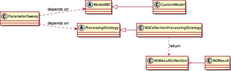 Figure 1
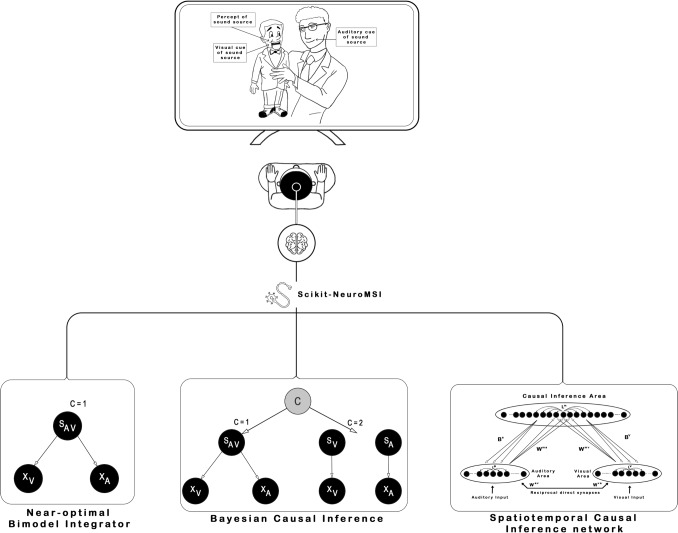 Figure 2
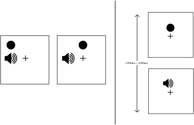 Figure 3
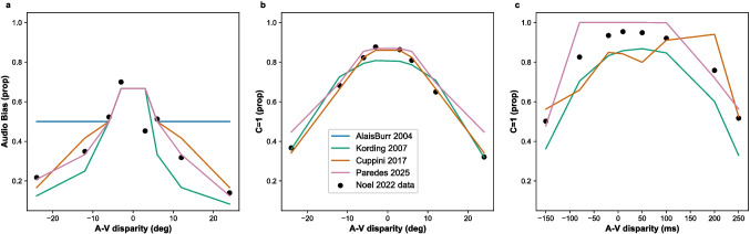 Figure 4
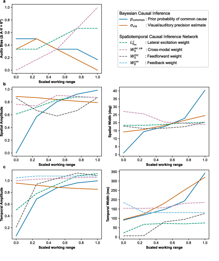 Figure 5
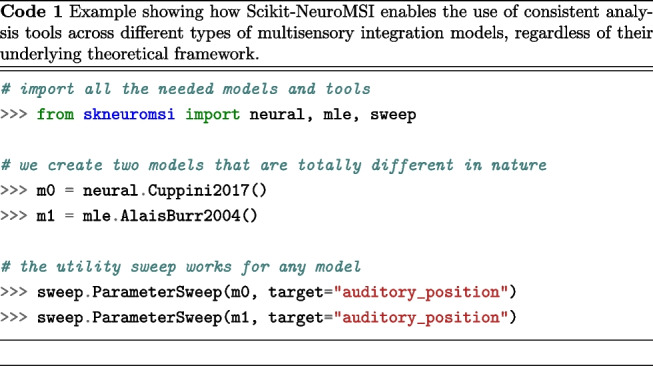 Figure 6
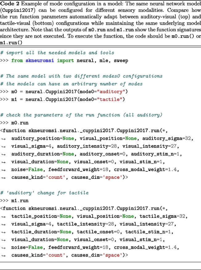 Figure 7
 Figure 8
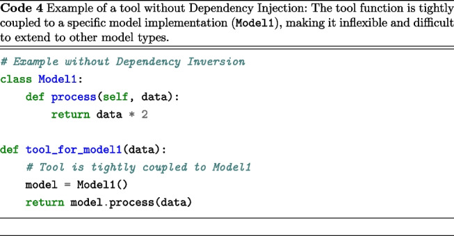 Figure 9
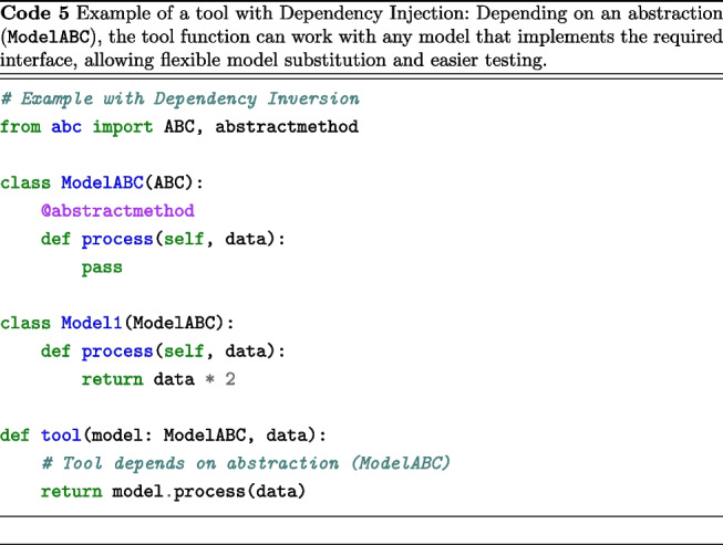 Figure 10
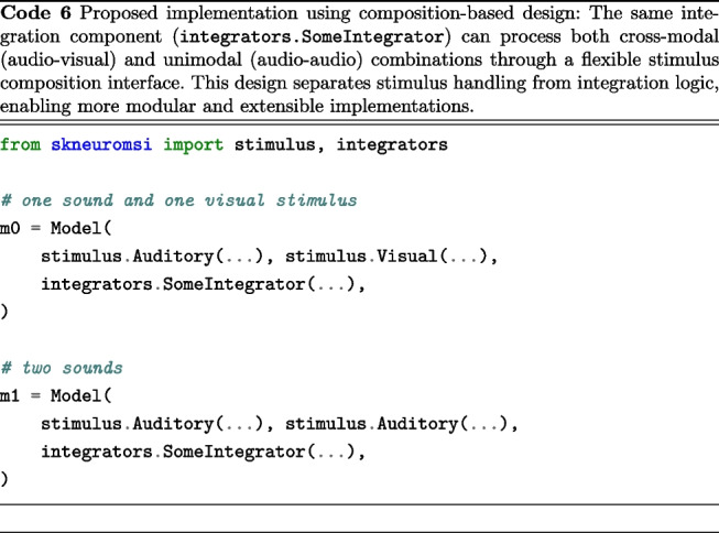 Figure 11
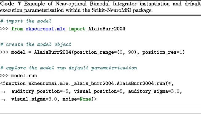 Figure 12
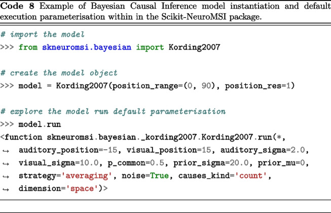 Figure 13
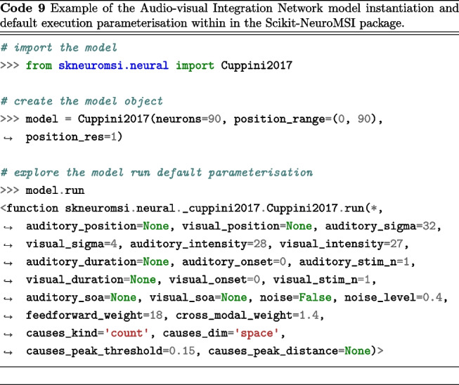 Figure 14
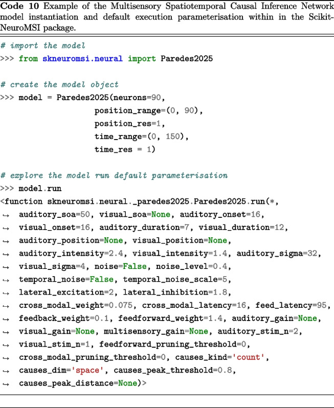 Figure 15
- —Pontificia Universidad Catolica del Peru
Peer Reviews
No public reviews on file for this paper yet. If you reviewed it on a platform where reviews are public (OpenReview, ICLR, NeurIPS, ICML), you can paste yours below so the community can read it here.
Videos
No videos yet. Explain this paper in a talk, walkthrough, or lecture? Add one.
Taxonomy
TopicsMultisensory perception and integration · Olfactory and Sensory Function Studies · Biochemical Analysis and Sensing Techniques
Introduction
Multisensory integration is the neural process by which signals originating from distinct sensory modalities (such as visual, tactile, or auditory) are merged. As a result, the multisensory response can differ significantly from the responses elicited by stimuli confined to a single sensory modality (Stein and Stanford, 2008; Stein et al., 2010). Disturbances in multisensory processing can impact various cognitive domains (Wallace et al., 2020). For example, alterations in multisensory function are observed in various neuropsychiatric and neurological disorders (e.g. SCZ, ASD, dementia, sensory loss, dyslexia) (Martin et al., 2013; Haßet al., 2017; Zvyagintsev et al., 2017; Paredes et al., 2022; Cascio et al., 2012; Stevenson et al., 2014; Hahn et al., 2014; Zhou et al., 2018; Noel et al., 2022a; Wu et al., 2012; Festa et al., 2017; Ramkhalawansingh et al., 2017). Furthermore, a substantial body of research is exploring the potential of multisensory markers to predict future clinical manifestations or to serve as key focal points for therapeutic interventions (Bolognini et al., 2005; Sánchez et al., 2013; Gieseler et al., 2018).
Computational modeling is crucial for the advancement of the field due to its potential to develop formal theories of the neural mechanisms of multisensory integration (Meijer and Noppeney, 2020; Colonius and Diederich, 2020). It forces scientists to analyze, specify, and formalize their ideas, while also allowing them to generate precise quantitative predictions suitable for testing in future experiments (Blohm et al., 2020; Guest and Martin, 2021). Consequently, the body of literature on computational models of multisensory integration has experienced substantial growth over the past two decades (Colonius and Diederich, 2020).
The main modeling approaches are optimal cue combination (Ernst and Banks, 2002; Alais and Burr, 2004; Fetsch et al., 2013; Parise and Ernst, 2016), Bayesian causal inference (Körding et al., 2007; Shams and Beierholm, 2010; Rohe and Noppeney, 2015; Rohe et al., 2019; Meijer and Noppeney, 2020), race (Diederich, 1992, 1995; Colonius and Diederich, 2004; Colonius et al., 2017), and network (Ma and Pouget, 2008; Ma and Rahmati, 2013; Ohshiro et al., 2011; Miller et al., 2017; Cuppini et al., 2017; Ursino et al., 2019) models. Despite being based on very general mechanisms, these models are typically restricted to a specific experimental paradigm (e.g. spatial localization, orientation judgments, temporal order judgments, rate detection, sound-induced flash illusion, among others) and vary in their level of description (e.g. computation, implementation or algorithm) and sophistication.
Overall, the field lacks a unified theoretical approach to multisensory integration that allows for model testing in different experimental and computational paradigms. There is a growing need for scientific software specifically designed to represent the distinctive concepts and mechanisms that characterize the integration of information from different sensory modalities. To our knowledge, there is as yet no software that can provide a unified computational environment designed to facilitate the examination of differences in model predictions. Multisensory integration modelers currently rely on packages built for general-purpose computational neuroscience modeling, such as Brian Stimberg et al. (2019), HDDM (Wiecki et al., 2013), TAPAS (Frässle et al., 2021) or PyRates (Gast et al., 2019), BrainPy (Wang et al., 2023), among others. There are also alternatives for specific multisensory integration models, such as the Bayesian Causal Inference Toolbox (Zhu et al., 2024a), but no frameworks encompassing more than one modeling approach.
Here we present Scikit-NeuroMSI (Paredes et al., 2023), an open-source Python (Rossum and Drake, 2010) framework that simplifies the implementation of neurocomputational models of multisensory integration. The package currently allows to run seminal computational models of multisensory integration and to easily implement new models defined by users. As an illustration, we show how this framework facilitates the analysis of spatiotemporal multisensory integration at different levels of description using Bayesian and network models.
This paper targets a diverse audience in neuroscience and computational fields, including computational neuroscientists and researchers in sensory processing. It is also beneficial for software developers and engineers interested in multisensory integration models. While basic neuroscience and programming knowledge is useful, proficiency in Python is needed to understand the implementation of Scikit-NeuroMSI, as it is developed in this language. We make the paper accessible by covering theoretical foundations and practical implementations, with explanations and code examples to aid comprehension. Those with Python skills can dive directly into the implementation details, while newcomers will find enough context to grasp the concepts. This approach highlights the challenge of standardizing multisensory integration models, which requires a blend of neuroscience, mathematics, and software engineering.
Software
Design Overview
Experiments on multisensory integration investigate how the brain combines information from multiple sensory modalities to create a unified perception of the environment. These studies often involve manipulating the reliability or congruency of sensory cues from different modalities, such as vision and touch, to examine how the brain weighs and integrates this information (Colonius and Diederich, 2020). Experimental paradigms include spatial localisation tasks for cross-modal spatial interactions (Ernst and Banks, 2002; Alais and Burr, 2004), temporal order judgments for timing perception of multisensory events (Ferri et al., 2016), or the double flash illusion for auditory influence on visual perception (Shams et al., 2002), among others.
Computational models play a crucial role in multisensory research by providing frameworks to predict and explain behavioral and neural responses in multisensory contexts (Chandrasekaran, 2017). These models help researchers understand the underlying principles of sensory integration, such as reliability-based cue weighting and inverse effectiveness (Stein et al., 2020). By comparing model predictions with empirical data, researchers can test hypotheses about the neural mechanisms of multisensory integration and gain insights into how the brain creates coherent perceptions from diverse sensory inputs (Blohm et al., 2020).
A wide range of computational models for multisensory integration is available (Colonius and Diederich, 2020), providing descriptions at computational, algorithmic, and implementation levels within information-processing theory (Marr, 2010). Nevertheless, it is unusual to find formal evaluations of multisensory integration using more than one model at the time to bridge across levels of analysis (Ursino et al., 2014).
Scikit-NeuroMSI was designed to meet three fundamental requirements in the computational study of multisensory integration:
- Modeling Standardization: Researchers need to compare different theoretical approaches (Bayesian, neural network, maximum likelihood estimation, among others) using consistent analysis methods. Our framework provides a standardized interface for implementing and analyzing different types of models.
- Data Processing Pipeline: The framework handles multidimensional data processing across:
- Spatial dimensions (1D to 3D spatial coordinates)
- Temporal sequences
- Multiple sensory modalities (e.g., visual, auditory, touch)
- Analysis Tools: We provide integrated tools for:
- Parameter sweeping across model configurations
- Result visualisation and export
- Statistical analysis of model outputs Furthermore, the software processes fundamental attributes of experimental inputs pertinent to multisensory research: spatial coordinates (e.g., degrees of visual angle and sound source location), temporal properties (encompassing stimulus onset, duration, and inter-stimulus intervals), stimulus intensity, and spatiotemporal reliability (random noise). Each input is validated to ensure compliance with the formatting standards, followed by a transformation to standardized internal representations that facilitate effective model processing. The software systematically applies type checking and data validation protocols to ensure the integrity of the inputs before proceeding with processing.
Consequently, the software requires a uniform output for each multisensory integration model. This output incorporates the activity values from all participating modalities, necessitating at least two unisensory modes along with one multisensory mode. There is an optional provision for output related to causal inference responses, as determined by the user. These prerequisites guided the technical design choices detailed in the next section.
A Formal and Technical Approach for the Model Standardization
We outline the theoretical and mathematical basis of multisensory integration models. We first describe the formal properties and mathematical framework needed to understand these computational problems theoretically, which aids in addressing software engineering challenges. Our development of Scikit-NeuroMSI aimed to articulate these problems with minimal conceptual differences, removing programming overhead to focus on solving multisensory integration issues (Brooks and Kugler, 1987). Specific implementation details and practical considerations are discussed in Section “Implemented Models", with examples of applying these principles in the software framework.
Computational Model Formalities
This work aims to create a unified framework for multisensory integration models (Colonius and Diederich, 2020) through Scikit-NeuroMSI, facilitating interoperability between analysis, comparison, and explanation tools, regardless of the specific model.
Consider two distinct model outputs r0 and r1, such as Bayesian models (Körding et al., 2007; Shams and Beierholm, 2010), neural networks (Cuppini et al., 2014, 2017), or maximum likelihood estimators (Ernst and Banks, 2002; Alais and Burr, 2004), with different modalities and dimensions. Any processing function f should handle both r0 and r1 equally well.
In general, our goal is to create models (m) that produce results (r) compatible with any processing function f, ensuring that the new m or f are mutually compatible (see Appendix A for a mathematical formulation). For example, Code 1 shows that neural network models (Cuppini et al., 2017) and maximum likelihood estimation models (Alais and Burr, 2004) can be analyzed with the same parameter sweep tools.
Another goal was to allow users to choose the sensory modality they simulate, reflecting real-world scenarios. For example, a researcher might study visual-auditory stimuli interaction in one experiment and visual-tactile in another. This allows models to adapt parameters to dynamically match selected modalities. As demonstrated in Code 2 an audio-visual setup reveals parameters such as "auditory_position", while a visual-tactile setup replaces them with parameters such as "tactile_position", keeping the core model structure and logic intact.
The final design requirement ensures multidimensional analysis of data. Each model output point is associated with a specific mode, time, and space, with the spatial dimension possibly encompassing one to three dimensions. Consequently, the model output can comprise up to five dimensions (5D).
Object-Oriented Design
Selecting an ecosystem for a tool is a subjective decision. Most data analysis projects use Python due to its rich scientific ecosystem (Perez et al., 2010). We chose Python to exploit object-oriented mechanisms, enhancing simplicity and tool extensibility. In object-oriented languages such as Python, classes structure data types by grouping attributes (state) and methods (behavior), enabling cohesive code organization and providing inheritance for sharing functionalities without code duplication (Booch, 1982).
A conceptual mechanism available in object-oriented programming languages that we employed is abstract classes. These represent data types that, although possessing a complete protocol (i.e., their functions, the data they receive, and the return types are fully defined), have certain behaviors that remain unspecified. For example, as demonstrated in Code 3, the Foo class utilizes the functionality already established in the method0() method without necessitating redundancy in the source code. Furthermore, this establishes a hierarchical structure, or inheritance, between the FooABC and Foo types, indicating that any object created or instantiated by Foo is an instance of the FooABC type. The final aspect to note is that FooABC is explicitly declared as an incomplete entity and is thus non-instantiable, achieved by adorning method1() with @abstractmethod.
We followed the “Dependency Inversion Principle” (DIP), an essential SOLID principle (Martin, 2000), which establishes two fundamental rules:
- High-level modules should not depend on low-level modules. Both should depend on abstractions.
- Abstractions should not depend on details. Details should depend on abstractions. To illustrate its importance, we compare two model processing tool implementations. Code 4 is tightly coupled, relying directly on a specific model, while Code 5 is more flexible, using dependency injection via an abstract base class.
The main distinction between these methodologies lies in that Code 4 contains a tool function specifically hardcoded to operate solely with Model1, thereby precluding its application to other model types unless the function is modified. In contrast, Code 5 is designed to accommodate any model inheriting from ModelABC, facilitating the seamless integration of new model types, allowing runtime model substitution, enhancing testability through mock objects, and ensuring a more robust separation of concerns. This pattern is essential for Scikit-NeuroMSI, as it enables the consistent implementation of tools across various multisensory integration models.
We propose a set of classes to reduce the “semantic gap” that separates the ideas of how a multisensory integration problem is expressed and how the code that represents these ideas is written. Two main classes form the core architecture of the framework:
- ModelABC: An abstract base class that defines the standard interface for all multisensory integration models
- NDResult: A result object responsible for storing multidimensional stimulus information and providing analysis tools for research This two-class design separates the model implementation logic from the data handling and analysis capabilities, following standard software engineering principles. The entirety of the classes, along with their interconnections, is presented in a diagram employing UML language (Jacobson et al., 2000) to formally depict the relationships among the core modules of the project (see Fig. 1).Fig. 1Reduced Class Diagram of Scikit-NeuroMSI. Empty arrows represent inheritance, the diamond-headed arrow indicates that multiple NDResult objects are aggregated into a single NDResultCollection, and all other relationships have explanatory labels
ParameterSweep is a tool for performing parameter sweeps over models, offering high flexibility and employing interchangeable strategies to process results, thereby enabling efficient memory management. NDResultCollection serves as an auxiliary class designed to aggregate and compress results into organized collections. This facilitates advanced functionalities, such as the analysis of spatiotemporal disparity effects. Furthermore, NDResultCollection is the standard output format of ParameterSweep when using the default Processing Strategy. For a complete description of the implemented classes, refer to Appendix B.
Implemented Models
Any model of multisensory integration must define the link between responses to unisensory signals, such as visual and auditory, and responses to cross-modal signals such as visual-auditory. This connection varies according to spatial and temporal characteristics, experimental configuration, and level of description (e.g. single neurons, neural populations, neuroimaging, behaviors). This opens a broad spectrum of approaches for modeling the observations derived from multisensory integration experiments.
A prevalent paradigm in this field is the Ventriloquist Effect (Thurlow and Jack, 1973). This phenomenon arises when incongruent visual and auditory stimuli are simultaneously presented, leading the observer to perceive a singular origin for both visual (the movements of a puppet’s face) and auditory (speech) stimuli, attributing them to the same source (the puppet’s speaking) (see Fig. 2 for an illustration). This effect is systematically investigated in laboratory environments through tasks designed to assess the spatial localization of an auditory source within a combined visual-auditory setting (Alais and Burr, 2004).Fig. 2Implemented models in Scikit-NeuroMSI. The illustration represents how the software package allows to model the Ventriloquist Effect (i.e. spatial integration under audio-visual disparities) using three different approaches: Near-optimal Bimodal Integrator, Bayesian Causal Inference and Spatiotemporal Causal Inference network
In general, these models aim to explain common “empirical rules” derived from multisensory integration paradigms (see Colonius and Diederich 2020 and Stein et al. 2020 for a detailed review). The “spatio-temporal rule” suggests that stimuli near in space and time are more likely to be integrated. The “inverse-effectiveness rule” states that integration is stronger when the unimodal input intensity decreases. Additionally, the “reliability rule” emphasizes a greater weighting of more reliable modalities (e.g., with lower noise). These empirically observed “rules” have been demonstrated to arise from common computational principles (Ohshiro et al., 2011) and do not necessarily require alternative models for their explanation. In consequence, the key challenge is the development of models capable of accounting for empirical observations of multisensory integration across various levels of description.
Here we present the main models of the Ventriloquist Effect currently available in the Scikit-NeuroMSI package. Appendix C contains a comprehensive mathematical exposition of the models, as well as the code necessary for their execution. The package currently includes models pertinent to additional paradigms, such as the Sound-Induced Flash Illusion (Cuppini et al., 2014; Zhu et al., 2024b). These models are not elaborated upon in depth in this article, but are thoroughly delineated in the user documentation. Furthermore, we provide guidance on how to streamline the incorporation of novel models into the package. We actively encourage the research community specializing in multisensory integration to contribute to this initiative by developing and sharing their own models (refer to Contributing Guidelines).
Near-Optimal Bimodal Integrator
An early model proposes that the process of cue combination from different modalities resembles a maximum-likelihood integrator (Ernst and Banks, 2002). The Near-optimal Bimodal Integrator (Alais and Burr, 2004) for auditory (A) and visual (V) signals in the context of an auditory spatial localization task (e.g. Ventriloquist effect) can be computed by adding the unisensory estimates ( \documentclass[12pt]{minimal} \usepackage{amsmath} \usepackage{wasysym} \usepackage{amsfonts} \usepackage{amssymb} \usepackage{amsbsy} \usepackage{mathrsfs} \usepackage{upgreek} \setlength{\oddsidemargin}{-69pt} \begin{document}$$\hat{S}_{A}$$\end{document} and \documentclass[12pt]{minimal} \usepackage{amsmath} \usepackage{wasysym} \usepackage{amsfonts} \usepackage{amssymb} \usepackage{amsbsy} \usepackage{mathrsfs} \usepackage{upgreek} \setlength{\oddsidemargin}{-69pt} \begin{document}$$\hat{S}_{V}$$\end{document} ) weighted by their reliability. Consequently, the integrated percept is predisposed to align more closely with the signal that exhibits lower variability.
Bayesian Causal Inference
In the previous model, cue integration is essential for accurately estimating a cross-modal stimulus. However, if there is a significant difference between the subjective assessments \documentclass[12pt]{minimal} \usepackage{amsmath} \usepackage{wasysym} \usepackage{amsfonts} \usepackage{amssymb} \usepackage{amsbsy} \usepackage{mathrsfs} \usepackage{upgreek} \setlength{\oddsidemargin}{-69pt} \begin{document}$$\hat{S}_{A}$$\end{document} and \documentclass[12pt]{minimal} \usepackage{amsmath} \usepackage{wasysym} \usepackage{amsfonts} \usepackage{amssymb} \usepackage{amsbsy} \usepackage{mathrsfs} \usepackage{upgreek} \setlength{\oddsidemargin}{-69pt} \begin{document}$$\hat{S}_{V}$$\end{document} from a visual-auditory stimulus, the observer cannot determine if this difference is due to random noise in neural signal processing or systematic signal divergence.
Originally designed to explain the Ventriloquist Effect, the Bayesian Causal Inference model (Körding et al., 2007) distinguishes whether \documentclass[12pt]{minimal} \usepackage{amsmath} \usepackage{wasysym} \usepackage{amsfonts} \usepackage{amssymb} \usepackage{amsbsy} \usepackage{mathrsfs} \usepackage{upgreek} \setlength{\oddsidemargin}{-69pt} \begin{document}$$\hat{S}_{A}$$\end{document} and \documentclass[12pt]{minimal} \usepackage{amsmath} \usepackage{wasysym} \usepackage{amsfonts} \usepackage{amssymb} \usepackage{amsbsy} \usepackage{mathrsfs} \usepackage{upgreek} \setlength{\oddsidemargin}{-69pt} \begin{document}$$\hat{S}_{V}$$\end{document} arise from a single audiovisual event (integration) or separate events (segregation). To do so, the observer considers the likelihood of \documentclass[12pt]{minimal} \usepackage{amsmath} \usepackage{wasysym} \usepackage{amsfonts} \usepackage{amssymb} \usepackage{amsbsy} \usepackage{mathrsfs} \usepackage{upgreek} \setlength{\oddsidemargin}{-69pt} \begin{document}$$\hat{S}_{A}$$\end{document} and \documentclass[12pt]{minimal} \usepackage{amsmath} \usepackage{wasysym} \usepackage{amsfonts} \usepackage{amssymb} \usepackage{amsbsy} \usepackage{mathrsfs} \usepackage{upgreek} \setlength{\oddsidemargin}{-69pt} \begin{document}$$\hat{S}_{V}$$\end{document} given a common or separate event and the prior probability of a common source. A higher likelihood occurs if the two unisensory signals are similar, which in turn increases the probability of inferring that the signals have a common cause.
Network Model for Audio-Visual Integration and Causal Inference
Bayesian causal inference models provide a high-level description (i.e. computational level of analysis according to Marr (Marr, 2010)) of the computations carried out by the brain to integrate unisensory signals. Recently, neural network models have been proposed as an alternative to model causal inference in multisensory integration paradigms (Cuppini et al., 2017; Fang et al., 2019; Rideaux et al., 2021), providing a low-level description of such a mechanism.
The audio-visual integration and causal inference network (Cuppini et al., 2017) features two unisensory regions for processing noisy auditory and visual stimuli, interconnected by cross-modal excitatory synapses. Here, rate-coded neurons are spatially organized, with closer neurons responding to nearer spatial positions. These regions emulate sensory processing in the brain’s unisensory cortex and determine the spatial location of the stimuli by computing the barycenter of activity in the auditory and visual regions. Cross-modal connections cause the spatial localization of one modality to be influenced by the concurrent presentation in another, even if processed separately.
Multisensory Spatiotemporal Causal Inference Network
Our research group developed the Multisensory Spatiotemporal Causal Inference Network to account for the sound-induced flash illusion (Paredes et al., 2025). This model was built upon preceding network models for spatial (Cuppini et al., 2017) and temporal (Cuppini et al., 2014) multisensory integration to inform two levels of causal inference processing. Our model consists of three layers: two encode auditory and visual stimuli separately and connect to a multisensory layer via feedforward and feedback synapses. At the unisensory areas, the model computes the spatiotemporal position of the external stimuli. In addition, at the multisensory area the model computes causal inference. This neural architecture allows iterative computation of spatiotemporal causal inference across the network (Rohe et al., 2019).Fig. 3Causal inference tasks. The figure shows the causal inference tasks reported in Noel et al. (2022b) that were simulated in this study. Left panel: Spatial audio-visual disparity task. Participants viewed a visual disk and heard an auditory tone at different locations and with different small disparities (top = no disparity, bottom = small disparity). We present each model with an auditory stimuli at a fixed position (45°) and visual stimuli at different positions relative to the auditory cue: ±3, ±6, ±12, and ±24°. The models had to determine the position of the auditory stimuli and report the number of causes (1 or 2). Right panel: Temporal audio-visual disparity task. Participants viewed a visual disk and heard an auditory stimuli at different onsets relative to the visual cue. We present each model with a visual stimulus at a fixed onset (160 ms) and auditory stimuli at different onsets relative to the visual cue: 0, ±20, ±80, ±150, and +250 ms. The models had to determine the number of causes of the stimuli (1 or 2)
In summary, our model retains neural connectivity (lateral, cross-modal, feedforward) and inputs as detailed in the previously discussed network (Cuppini et al., 2017), while integrating feedback connectivity. Additionally, this model introduces latency into the cross-modal and feed-forward-feedback neural inputs in accordance with literature indicating that early and late interactions during multisensory processing. Furthermore, in line with Cuppini et al. (2014), temporal filters have been incorporated for auditory, visual, and multisensory neurons to replicate the temporal progression of neural input and synaptic dynamics. These filters account for specific time constants that determine the temporal characteristics of each group of neurons, namely auditory, visual, or multisensory.
Example Applications
Modeling Spatiotemporal Causal Inference with Scikit-NeuroMSI
Causal inference is a highly relevant computation for multisensory integration (Körding et al., 2007; Shams and Beierholm, 2010, 2022). Causal inference in multisensory integration is examined through implicit or explicit tasks. Explicit causal inference involves tasks in which participants are required to directly assess the causal relationship between stimuli (unity judgment) in a multisensory setting, whereas implicit causal inference involves tasks where participants are required to estimate the spatiotemporal location of the stimuli. An in-depth investigation of how the causal mechanism operates in both types of tasks is currently in progress (Acerbi et al., 2018) and has been found to be distinct in neurodiverse populations (e.g. Noel et al. (2022b)).
In general, multisensory causal inference models rely mainly on Bayesian inference (Körding et al., 2007), offering a high-level description (as described by Marr’s computational level (Marr, 2010)) of how the brain integrates sensory signals (French and DeAngelis, 2020). Recently, neural network models have emerged as an alternative for modeling causal inference in multisensory contexts (Cuppini et al., 2017; Fang et al., 2019; Rideaux et al., 2021), providing a tentative implementation of the mechanism. Yet, these models have not been rigorously tested across multiple experimental frameworks or dimensions (i.e. space and time), nor have they been compared with other models. In the following, we ask: 1) Are the probabilistic and network models comparable in their performance when fitting data? 2) Do these models accurately account for both implicit and explicit causal inference responses? 3) Do these models show performance differences when working with spatial or temporal disparities?
Modeling Setup
We used the models currently implemented in Scikit-NeuroMSI to reproduce human responses in audio-visual causal inference tasks (see Experiments 2, 3 and 4 in Noel et al. (2022b) for details on the experimental setup) and qualitatively compared their performance. For each task, we fitted the implemented models to behavioral responses of healthy control participants using the differential evolution algorithm (Storn and Price, 1997) available in the SciPy library for the Python programming language (Virtanen et al., 2020). Details about the fitting procedure and model readout for each task can be found in the Appendix D.Fig. 4Models of audio-visual causal inference tasks. The figure shows optimal responses of the implemented models in multisensory causal inference in the audio-visual disparity tasks reported in Noel et al. (2022b). (a) Performance of the models in spatial localization within an implicit causal inference task. This graph reveals that Bayesian and network models provide optimal performance, whereas the MLE model fails to reproduce audio-visual disparities beyond ±6°. (b) Performance of the models in common source reports under spatial disparities within an explicit causal inference task. These simulations show that the network models outperform the Bayesian Causal Inference model in audio-visual spatial disparities below ±6°. (c) Performance of the models in common source reports under temporal disparities within an explicit causal inference task. This graph shows that both the Multisensory Spatiotemporal Causal Inference Network and the Bayesian Causal Inference models provide fair approximations to human performance, whereas the network model for audio-visual integration fails to reproduce disparities beyond ±100 ms
First, we model an auditory spatial localization task with disparate visual cues (Experiment 2 in Noel et al. (2022b)) to examine the implicit causal inference performance of the models. Our main focus is the modulation of auditory spatial perception by visual stimuli, a phenomenon known as auditory bias. We present each model with an auditory stimuli at a fixed position (45°) and visual stimuli at different positions relative to the auditory cue: ±3, ±6, ±12, and ±24°(see Fig. 3, left). For simplicity, we present each possible combination of audio-visual stimuli only once, and all noise sources are eliminated for this approach. Following Körding et al. (2007) and Cuppini et al. (2017), we compute the auditory bias as the spatial disparity between the position of the auditory stimulus and the position detected by each model, divided by the distance between the auditory and visual stimuli. We fit the auditory bias responses of the model to correspond with human responses under the high visual cue reliability condition (see Noel et al. 2022b for details).
Next, we model an audio-visual common cause report task under spatial disparities (Experiment 3 in Noel et al. (2022b)) to examine the explicit causal inference performance of the models. Audio-visual stimuli are delivered to each model at the same positions as in the previous simulation. Here, our focus is the modulation of the unity judgments (common cause reports) of the models by the spatial disparity of the stimuli. For the Bayesian model, we determine the proportion of reports indicating a common cause by calculating the posterior probability of a common cause (refer to Eq. C7). In contrast, for network models, this proportion is identified through the maximal neural activation (refer to Eq. C9) observed within the multisensory neurons.
Finally, we model an audio-visual common cause report task under temporal disparities (Experiment 4 in Noel et al. (2022b)) to examine the explicit temporal causal inference performance of the models. Here our focus is on how temporal disparities in stimuli affect the unity judgments of the models. We present each model with a visual stimulus at a fixed onset (160 ms) and auditory stimuli at different onsets relative to the visual cue: 0, ±20, ±80, ±150, and +250 ms (see Fig. 3, right). Each possible combination of audio-visual stimuli is presented only once, and all noise sources are eliminated for this approach. We calculate the proportions of the common cause reports of the models as in the previous simulation.
Simulation Results
We compared the performance of the implemented models in the aforementioned causal inference tasks. Auditory bias responses are shown in Fig. 4a. We observe that both Bayesian (Körding et al., 2007) and Network models (Cuppini et al., 2017) provide a good approximation to behavioral data, while the maximum likelihood estimation model (MLE) (Alais and Burr, 2004) fails to reproduce audio-visual disparities beyond ±6°.
Furthermore, spatial causal inference responses are shown in Fig. 4b. We observe that all the evaluated models provide a fair approximation to behavioral responses, with the neural network models (Cuppini et al., 2017) outperforming the Bayesian Causal Inference model (Körding et al., 2007) in audio-visual disparities below ±6°.
Temporal causal inference responses are shown in Fig. 4c. We observe that both the Bayesian Causal Inference model (Körding et al., 2007) and the Multisensory Spatiotemporal Causal Inference Network (Paredes et al., 2025) provide a good approximation to behavioral responses, whereas the network model for audio-visual integration (Cuppini et al., 2017) fails to reproduce temporal disparities beyond ±100 ms.
The findings from the current series of simulations indicate that the Bayesian Causal Inference and Spatiotemporal Causal Inference network models offer the most accurate representation of the participants’ data. However, the efficacy of both models diminishes when addressing temporal disparities, underscoring the need for new models that effectively incorporate causal inference within the temporal domain.
Comparing network and Bayesian models of Spatiotemporal Causal Inference with Scikit-NeuroMSI
To our knowledge, this is the first time that implicit and explicit spatiotemporal causal inference is computationally modeled using a combined Bayesian and Neural Network approach (Ursino et al., 2014; Acerbi et al., 2018). This methodology facilitates the concurrent assessment of the influence of each model parameter and the identification of similarities among them. We are now equipped to conduct comprehensive sweeps of parameters within each model and assess their effects on model responses to discern commonalities that may allow us to bridge both levels of description. This process enables the exploration of interindividual variability by combining different modeling approaches, offering new ways to study multisensory integration differences seen in psychiatric or neurological conditions (Martin et al., 2013; Haßet al., 2017; Zvyagintsev et al., 2017; Paredes et al., 2022; Cascio et al., 2012; Stevenson et al., 2014; Hahn et al., 2014; Zhou et al., 2018; Noel et al., 2022a; Wu et al., 2012; Festa et al., 2017; Ramkhalawansingh et al., 2017). In the following, we ask: 1) What would the correlates of the components of Bayesian models be in a more neural implementation? 2) Do the parameters of each model have the same impact on implicit and explicit causal inference responses? 3) Are the effects of model parameters the same for tasks involving spatial or temporal disparities?
Modeling Setup
For the Bayesian Causal Inference model, we explored the impact of varying the prior probability of a common cause ( \documentclass[12pt]{minimal} \usepackage{amsmath} \usepackage{wasysym} \usepackage{amsfonts} \usepackage{amssymb} \usepackage{amsbsy} \usepackage{mathrsfs} \usepackage{upgreek} \setlength{\oddsidemargin}{-69pt} \begin{document}$$p_{common}$$\end{document} ) and the precision of the unisensory estimates ( \documentclass[12pt]{minimal} \usepackage{amsmath} \usepackage{wasysym} \usepackage{amsfonts} \usepackage{amssymb} \usepackage{amsbsy} \usepackage{mathrsfs} \usepackage{upgreek} \setlength{\oddsidemargin}{-69pt} \begin{document}$$\sigma _{a}$$\end{document} or \documentclass[12pt]{minimal} \usepackage{amsmath} \usepackage{wasysym} \usepackage{amsfonts} \usepackage{amssymb} \usepackage{amsbsy} \usepackage{mathrsfs} \usepackage{upgreek} \setlength{\oddsidemargin}{-69pt} \begin{document}$$\sigma _{v}$$\end{document} ). For Spatiotemporal Causal Inference network model, we explored the impact of manipulating the weights of cross-modal ( \documentclass[12pt]{minimal} \usepackage{amsmath} \usepackage{wasysym} \usepackage{amsfonts} \usepackage{amssymb} \usepackage{amsbsy} \usepackage{mathrsfs} \usepackage{upgreek} \setlength{\oddsidemargin}{-69pt} \begin{document}$$W_{0}^{av,va}$$\end{document} ), feedforward ( \documentclass[12pt]{minimal} \usepackage{amsmath} \usepackage{wasysym} \usepackage{amsfonts} \usepackage{amssymb} \usepackage{amsbsy} \usepackage{mathrsfs} \usepackage{upgreek} \setlength{\oddsidemargin}{-69pt} \begin{document}$$W_{0}^{mc}$$\end{document} ), feedback ( \documentclass[12pt]{minimal} \usepackage{amsmath} \usepackage{wasysym} \usepackage{amsfonts} \usepackage{amssymb} \usepackage{amsbsy} \usepackage{mathrsfs} \usepackage{upgreek} \setlength{\oddsidemargin}{-69pt} \begin{document}$$W_{0}^{cm}$$\end{document} ) and excitatory lateral ( \documentclass[12pt]{minimal} \usepackage{amsmath} \usepackage{wasysym} \usepackage{amsfonts} \usepackage{amssymb} \usepackage{amsbsy} \usepackage{mathrsfs} \usepackage{upgreek} \setlength{\oddsidemargin}{-69pt} \begin{document}$$L_{0_{ex}}^{c}$$\end{document} ) synapses. These parameters were selected due to its relevance in explaining individual differences in multisensory integration found in psychiatric conditions, as shown by recent computational research (Karvelis et al., 2018; Noel et al., 2022a, b; Paredes et al., 2022; Chrysaitis and Seriès, 2023; Noel and Angelaki, 2023).
First, we explored the impact of manipulating these parameters on the auditory bias responses of the selected models in the implicit causal inference task (Experiment 2 in Noel et al. (2022b)). For simplicity, we computed the auditory bias at the -6°disparity point for each value of the explored parameters. Next, we examined the effects of sweeping parameters on the proportion of synchronous reports across spatial and temporal disparities (Experiments 3 and 4 in Noel et al. (2022b)). Following Noel et al. (2022b), these differences were systematically quantified by fitting Gaussian functions to the proportion of common source responses as a function of audio-visual disparities ( \documentclass[12pt]{minimal} \usepackage{amsmath} \usepackage{wasysym} \usepackage{amsfonts} \usepackage{amssymb} \usepackage{amsbsy} \usepackage{mathrsfs} \usepackage{upgreek} \setlength{\oddsidemargin}{-69pt} \begin{document}$$\Delta $$\end{document} ). The Gaussian fits provide three parameters that characterize the responses of the computational models: (1) amplitude, denoting the maximum proportion of common source reports by the model; (2) mean, indicating the \documentclass[12pt]{minimal} \usepackage{amsmath} \usepackage{wasysym} \usepackage{amsfonts} \usepackage{amssymb} \usepackage{amsbsy} \usepackage{mathrsfs} \usepackage{upgreek} \setlength{\oddsidemargin}{-69pt} \begin{document}$$\Delta $$\end{document} at which the proportion of common source reports was maximal; and (3) width (standard deviation), reflecting the extent of \documentclass[12pt]{minimal} \usepackage{amsmath} \usepackage{wasysym} \usepackage{amsfonts} \usepackage{amssymb} \usepackage{amsbsy} \usepackage{mathrsfs} \usepackage{upgreek} \setlength{\oddsidemargin}{-69pt} \begin{document}$$\Delta $$\end{document} within which the model was prone to report a common source.
Simulation Results
The simulated auditory bias responses are shown in Fig. 5a. We found that both \documentclass[12pt]{minimal} \usepackage{amsmath} \usepackage{wasysym} \usepackage{amsfonts} \usepackage{amssymb} \usepackage{amsbsy} \usepackage{mathrsfs} \usepackage{upgreek} \setlength{\oddsidemargin}{-69pt} \begin{document}$$p_{common}$$\end{document} and \documentclass[12pt]{minimal} \usepackage{amsmath} \usepackage{wasysym} \usepackage{amsfonts} \usepackage{amssymb} \usepackage{amsbsy} \usepackage{mathrsfs} \usepackage{upgreek} \setlength{\oddsidemargin}{-69pt} \begin{document}$$\sigma _{v}$$\end{document} within the Bayesian framework are inversely related to \documentclass[12pt]{minimal} \usepackage{amsmath} \usepackage{wasysym} \usepackage{amsfonts} \usepackage{amssymb} \usepackage{amsbsy} \usepackage{mathrsfs} \usepackage{upgreek} \setlength{\oddsidemargin}{-69pt} \begin{document}$$L_{0_{ex}}^{c}$$\end{document} and \documentclass[12pt]{minimal} \usepackage{amsmath} \usepackage{wasysym} \usepackage{amsfonts} \usepackage{amssymb} \usepackage{amsbsy} \usepackage{mathrsfs} \usepackage{upgreek} \setlength{\oddsidemargin}{-69pt} \begin{document}$$W_{0}^{av,va}$$\end{document} within the network level. In line with previous network modeling of audiovisual integration (Ursino et al., 2017, 2019), our results suggest a possible neural correlate of the prior probability of the co-occurrence of audio-visual stimuli in the cross-modal synapses, with such neural mechanism impacting unisensory precision as well.
In addition, the simulated common source responses in the spatial causal inference task are shown in Fig. 5b. We found that \documentclass[12pt]{minimal} \usepackage{amsmath} \usepackage{wasysym} \usepackage{amsfonts} \usepackage{amssymb} \usepackage{amsbsy} \usepackage{mathrsfs} \usepackage{upgreek} \setlength{\oddsidemargin}{-69pt} \begin{document}$$\sigma _{v}$$\end{document} within the Bayesian model shows an opposite impact in the amplitude and width of the common source reports compared to \documentclass[12pt]{minimal} \usepackage{amsmath} \usepackage{wasysym} \usepackage{amsfonts} \usepackage{amssymb} \usepackage{amsbsy} \usepackage{mathrsfs} \usepackage{upgreek} \setlength{\oddsidemargin}{-69pt} \begin{document}$$W_{0}^{av,va}$$\end{document} at the network level. This highlights the impact of cross-modal connectivity in explicit causal inference judgments, suggesting that its observed association with sensory precision estimates potentially scale up towards higher order cortical areas responsible for causal inference computations (Rohe and Noppeney, 2015; Rohe et al., 2019).
The simulated common source responses in the temporal causal inference task are shown in Fig. 5c. In contrast to observations in the spatial domain, we found that the \documentclass[12pt]{minimal} \usepackage{amsmath} \usepackage{wasysym} \usepackage{amsfonts} \usepackage{amssymb} \usepackage{amsbsy} \usepackage{mathrsfs} \usepackage{upgreek} \setlength{\oddsidemargin}{-69pt} \begin{document}$$p_{common}$$\end{document} within the Bayesian model displays a similar impact in the amplitude and width of the common source reports compared to \documentclass[12pt]{minimal} \usepackage{amsmath} \usepackage{wasysym} \usepackage{amsfonts} \usepackage{amssymb} \usepackage{amsbsy} \usepackage{mathrsfs} \usepackage{upgreek} \setlength{\oddsidemargin}{-69pt} \begin{document}$$W_{0}^{mc}$$\end{document} at the network level. This discrepancy opens up questions about potential differences in the mechanisms driving temporal and spatial causal inference, or at the very least, in the foundational assumptions under which these models were initially formulated. Notably, most of the modeling efforts have been carried out in spatial (static) multisensory integration tasks, whereas models of causal inference in the temporal domain at different levels of description have recently begun to accumulate (Cuppini et al., 2014; Pesnot Lerousseau et al., 2022; Zhu et al., 2024b).Fig. 5. Impact of model parameters on causal inference responses in Bayesian and network models. (a) Parameter sweeps on the implicit causal inference task. The simulations indicate that the prior probability of a common cause ( \documentclass[12pt]{minimal} \usepackage{amsmath} \usepackage{wasysym} \usepackage{amsfonts} \usepackage{amssymb} \usepackage{amsbsy} \usepackage{mathrsfs} \usepackage{upgreek} \setlength{\oddsidemargin}{-69pt} \begin{document}$$p_{common}$$\end{document} ) and visual estimate precision ( \documentclass[12pt]{minimal} \usepackage{amsmath} \usepackage{wasysym} \usepackage{amsfonts} \usepackage{amssymb} \usepackage{amsbsy} \usepackage{mathrsfs} \usepackage{upgreek} \setlength{\oddsidemargin}{-69pt} \begin{document}$$\sigma _{v}$$\end{document} ) reduce auditory bias in the Bayesian model, while lateral excitation ( \documentclass[12pt]{minimal} \usepackage{amsmath} \usepackage{wasysym} \usepackage{amsfonts} \usepackage{amssymb} \usepackage{amsbsy} \usepackage{mathrsfs} \usepackage{upgreek} \setlength{\oddsidemargin}{-69pt} \begin{document}$$L_{0_{ex}}^{c}$$\end{document} ) and cross-modal weights ( \documentclass[12pt]{minimal} \usepackage{amsmath} \usepackage{wasysym} \usepackage{amsfonts} \usepackage{amssymb} \usepackage{amsbsy} \usepackage{mathrsfs} \usepackage{upgreek} \setlength{\oddsidemargin}{-69pt} \begin{document}$$W_{0}^{av,va}$$\end{document} ) enhance it in our network model. (b) Parameter sweeps on the explicit spatial causal inference task. The proportion of common source responses relative to spatial disparities fitted to a Gaussian function for analysis. The simulations show that in the Bayesian Causal Inference model the parameter \documentclass[12pt]{minimal} \usepackage{amsmath} \usepackage{wasysym} \usepackage{amsfonts} \usepackage{amssymb} \usepackage{amsbsy} \usepackage{mathrsfs} \usepackage{upgreek} \setlength{\oddsidemargin}{-69pt} \begin{document}$$\sigma _{v}$$\end{document} shows an opposite impact in the amplitude and width of the common source reports compared to \documentclass[12pt]{minimal} \usepackage{amsmath} \usepackage{wasysym} \usepackage{amsfonts} \usepackage{amssymb} \usepackage{amsbsy} \usepackage{mathrsfs} \usepackage{upgreek} \setlength{\oddsidemargin}{-69pt} \begin{document}$$W_{0}^{av,va}$$\end{document} in the model. (c) Parameter sweeps on the explicit temporal causal inference task. The simulations show that in the Bayesian model \documentclass[12pt]{minimal} \usepackage{amsmath} \usepackage{wasysym} \usepackage{amsfonts} \usepackage{amssymb} \usepackage{amsbsy} \usepackage{mathrsfs} \usepackage{upgreek} \setlength{\oddsidemargin}{-69pt} \begin{document}$$p_{common}$$\end{document} displays a similar impact in the amplitude and width of the common source reports compared to \documentclass[12pt]{minimal} \usepackage{amsmath} \usepackage{wasysym} \usepackage{amsfonts} \usepackage{amssymb} \usepackage{amsbsy} \usepackage{mathrsfs} \usepackage{upgreek} \setlength{\oddsidemargin}{-69pt} \begin{document}$$W_{0}^{mc}$$\end{document} in the network model
Overall, the Bayesian parameter \documentclass[12pt]{minimal} \usepackage{amsmath} \usepackage{wasysym} \usepackage{amsfonts} \usepackage{amssymb} \usepackage{amsbsy} \usepackage{mathrsfs} \usepackage{upgreek} \setlength{\oddsidemargin}{-69pt} \begin{document}$$p_{common}$$\end{document} representing prior beliefs about common causes could be mapped to neural parameters such as \documentclass[12pt]{minimal} \usepackage{amsmath} \usepackage{wasysym} \usepackage{amsfonts} \usepackage{amssymb} \usepackage{amsbsy} \usepackage{mathrsfs} \usepackage{upgreek} \setlength{\oddsidemargin}{-69pt} \begin{document}$$L_{0_{ex}}^{c}$$\end{document} , \documentclass[12pt]{minimal} \usepackage{amsmath} \usepackage{wasysym} \usepackage{amsfonts} \usepackage{amssymb} \usepackage{amsbsy} \usepackage{mathrsfs} \usepackage{upgreek} \setlength{\oddsidemargin}{-69pt} \begin{document}$$W_{0}^{av,va}$$\end{document} and \documentclass[12pt]{minimal} \usepackage{amsmath} \usepackage{wasysym} \usepackage{amsfonts} \usepackage{amssymb} \usepackage{amsbsy} \usepackage{mathrsfs} \usepackage{upgreek} \setlength{\oddsidemargin}{-69pt} \begin{document}$$W_{0}^{mc}$$\end{document} representing inter and intra-areal synaptic strengths, although no exact parallel could be found across domains (spatial or temporal) or metrics (bias, amplitude and width). Similarly, \documentclass[12pt]{minimal} \usepackage{amsmath} \usepackage{wasysym} \usepackage{amsfonts} \usepackage{amssymb} \usepackage{amsbsy} \usepackage{mathrsfs} \usepackage{upgreek} \setlength{\oddsidemargin}{-69pt} \begin{document}$$\sigma _{v/a}$$\end{document} representing uncertainty in sensory information could be inversely mapped to \documentclass[12pt]{minimal} \usepackage{amsmath} \usepackage{wasysym} \usepackage{amsfonts} \usepackage{amssymb} \usepackage{amsbsy} \usepackage{mathrsfs} \usepackage{upgreek} \setlength{\oddsidemargin}{-69pt} \begin{document}$$W_{0}^{av,va}$$\end{document} , reflecting the strength of cross-modal connectivity at the network level, due to their opposite impact in the amplitude and width of the common source reports during explicit tasks. The observed discrepancies, including the differing effects of Bayesian and network models on implicit versus explicit causal inference tasks, indicate the presence of additional neural complexities that may not be fully encapsulated by Bayesian modeling or, conversely, by network approaches. The acquired understanding of the similarities of these models opens up the possibility of extending the current theoretical accounts of multisensory integration (Colonius and Diederich, 2020).
Discussion
We have addressed the objective of developing scientific software specifically designed for the computational modeling of multisensory integration, attending a key necessity in the field (Colonius and Diederich, 2020; Shams and Beierholm, 2022). We demonstrated the capabilities of Scikit-NeuroMSI in facilitating the implementation of multisensory integration models and systematically investigating their behavior by sweeping parameters across simulations (see Code 1 and Fig. 4). We have also demonstrated the utility of the software by modeling spatiotemporal causal inference at different levels of analysis using Bayesian (Körding et al., 2007) and network models of multisensory integration (see Fig. 5), addressing a fundamental inquiry necessary for advancing the field (Ursino et al., 2014; French and DeAngelis, 2020; Shams and Beierholm, 2022).
With software tools such as a Scikit-NeuroMSI we are now able to approximate multisensory integration at different levels of analysis (Marr, 2010) (e.g. computational, algorithmic, and neural) simultaneously and extend our possibilities of generating computationally informed hypotheses. This enables the formulation of more precise predictions that can be evaluated with neurobiological and behavioral measurements, a factor crucial for the consolidation of emerging theories of multisensory integration in neuroscience (Colonius and Diederich, 2020; Shams and Beierholm, 2022).
An immediate application for our new modeling framework is the study of multisensory integration differences in psychiatric and neurological disorders (Martin et al., 2013; Haßet al., 2017; Zvyagintsev et al., 2017; Paredes et al., 2022; Cascio et al., 2012; Stevenson et al., 2014; Hahn et al., 2014; Zhou et al., 2018; Noel et al., 2022a; Wu et al., 2012; Festa et al., 2017; Ramkhalawansingh et al., 2017). For example, a novel quantitative theory on ASD (Noel and Angelaki, 2023) suggests that ASD could be interpreted as a multisensory causal inference disorder (computational level), where this process may be facilitated by divisive normalization (algorithmic level) and potentially disrupted by excitatory/inhibitory imbalances (neural implementation level). However, there is as yet no formal evaluation of experimental data of this disorder using more than one multisensory integration model at the time to bridge across levels of analysis.
We acknowledge that our modeling effort represents a first step towards achieving a general solution for multisensory integration formalization. We have shown the capabilities of our software in the simulation of multiple models in a group of three similar tasks (Noel et al., 2022b). However, our software framework requires the incorporation of model comparison and validation metrics to facilitate the critical assessment of each model implementation (Wilson and Collins, 2019; Blohm et al., 2020). Overall, we propose a software environment as a first approach to a generalized framework for multisensory integration, needed for the theoretical advancement of the field.
Availability and Future Directions
The entire source code is under a BSD 3-Clause License and available in a public repository: https://github.com/renatoparedes/scikit-neuromsi. Scikit-NeuroMSI is available for installation on the Python Package-Index (PyPI)1. User documentation is automatically generated from Scikit-NeuroMSI docstrings and published in the Read the Docs service2.
In Spanish, there is a phrase “Con el diario del Lunes” (literally, “With Monday’s newspaper”), which shares the same meaning as the English expression “Monday-morning quarterback” - indicating that something becomes obvious only after it has happened. While Scikit-NeuroMSI has successfully achieved its technical objective of standardizing existing multisensory integration models, our experience has revealed opportunities for improved computational modeling.
Specifically, the architecture could be enhanced by decomposing the models into two distinct entities:
- A stimulus processing component that handles individual sensory inputs
- An integration component that consolidates the results into a unified modality Or mathematically speaking:
Where:
- S represents the stimulus source(s) from one or multiple modalities
- I is the integrator that combines the stimuli from S We envision a Python implementation similar to what is presented in Code 6. By decoupling stimulus processing/generation from integration mechanisms, new integration models can be easily implemented and tested without modifying the underlying stimulus code. The flexible architecture simplifies the implementation of sophisticated integration strategies and enables straightforward extension to handle additional modalities or stimulus types, making the framework particularly valuable for emerging research in areas such as brain-computer interfaces and robotics. From a software perspective, this new design would promote code reusability and make the codebase more maintainable, allowing the scientific community to contribute new models and extensions to the framework more easily.
Information Sharing Statement
The code and data used to generate the simulations presented in this article is available at: https://github.com/renatoparedes/NeuroMSI-Network.
The reference list from the paper itself. Each links out to its DOI / PubMed record.
- 1Bolognini, N., Rasi, F., Coccia, M., Làdavas, E. (2005). Visual search improvement in hemianopic patients after audio-visual stimulation. Brain: A Journal of Neurology, 128(Pt 12), 2830–2842. 10.1093/brain/awh 65610.1093/brain/awh 65616219672 · doi ↗ · pubmed ↗
- 2Brooks, F., & Kugler, H. (1987). No silver bullet. April.
- 3Cascio, C.J., Foss-Feig, J.H., Burnette, C.P., Heacock, J.L., Cosby, A.A. (2012). The rubber hand illusion in children with autism spectrum disorders: delayed influence of combined tactile and visual input on proprioception. Autism: The International Journal of Research and Practice, 16(4), 406–419. 10.1177/136236131143040410.1177/1362361311430404 PMC 352918022399451 · doi ↗ · pubmed ↗
- 4Colonius, H., Wolff, F. H., & Diederich, A. (2017). Trimodal Race Model Inequalities in Multisensory Integration: I. Basics. Fron-tiers in Psychology,8, 1141. 10.3389/fpsyg.2017.0114110.3389/fpsyg.2017.01141 PMC 550419628744236 · doi ↗ · pubmed ↗
- 5Diederich, A. (1992). Intersensory facilitation: Race, superposition, and diffusion models for reaction time to multiple stimuli(vol. 369). Frankfurt am Main ; New York: Peter Lang.
- 6Gamma, E., Helm, R., Johnson, R., Vlissides, J., Patterns, D. (1995). Design patterns: Elements of reusable object-oriented software. Addison-Wesley.
- 7Gast, R., Rose, D., Salomon, C., Möller, H. E., Weiskopf, N., & Knösche, T. R. (2019). Py Rates—A Python framework for rate-based neural simulations. PLOS ONE,14(12), Article e 0225900. 10.1371/journal.pone.022590010.1371/journal.pone.0225900 PMC 691393031841550 · doi ↗ · pubmed ↗
- 8Haß, K., Sinke, C., Reese, T., Roy, M., Wiswede, D., Dillo, W., & Szycik, G. R. (2017). Enlarged temporal integration window in schizophrenia indicated by the double-flash illusion. Cognitive Neuropsychiatry,22(2), 145–158. 10.1080/13546805.2017.128769310.1080/13546805.2017.128769328253091 · doi ↗ · pubmed ↗