Rethinking Probability of Success as Bayes Utility
Fulvio De Santis, Stefania Gubbiotti, Francesco Mariani

TL;DR
This paper introduces a new way to define the probability of success in statistical trials using decision theory, aiming to improve accuracy and efficiency.
Contribution
The paper proposes a novel definition of probability of success based on expected utility, offering conceptual and practical advantages.
Findings
The new definition of PoS is based on the probability of making the correct hypothesis choice.
The proposed method can lead to smaller optimal sample sizes when the null hypothesis has non-zero probability.
Abstract
In the hybrid frequentist‐Bayesian approach, the probability of success (PoS) of a trial is the expected value of the traditional power function of a test with respect to a design prior assigned to the parameter under scrutiny. However, this definition is not univocal and some of the proposals do not lack of potential drawbacks. These problems are related to the fact that such definitions are all based on the probability of rejecting the null hypothesis rather than on the probability of choosing the correct hypothesis, be it the null or the alternative. In this article, we propose a unifying, decision‐theoretic approach that yields a new definition of PoS as the expected utility of the trial (u‐PoS), that is, as the expected probability of making the correct choice between the two hypotheses. This proposal shows a conceptual advantage over previous definitions of PoS; moreover, it…
Genes, proteins, chemicals, diseases, species, mutations and cell lines named across the full text — each resolved to its canonical identifier and authoritative record.
Click any figure to enlarge with its caption.
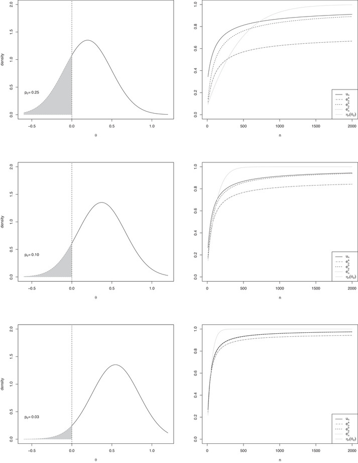 FIGURE 1
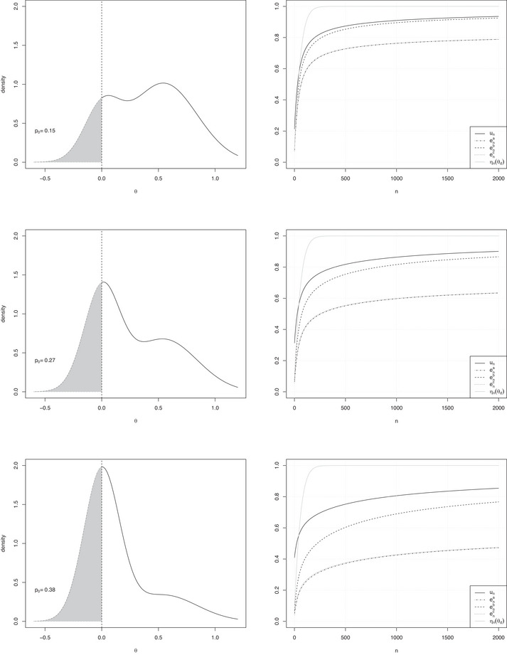 FIGURE 2
| Design prior | ||||||||
|---|---|---|---|---|---|---|---|---|
| 0.198 | 0 | 100 | 0.256 | 0.256 | 0.256 | 0.256 | ||
| 500 | 0.715 | 0.715 | 0.715 | 0.715 | ||||
| Point‐mass | 0.372 | 0 | 100 | 0.585 | 0.585 | 0.585 | 0.585 | |
| 500 | 0.994 | 0.994 | 0.994 | 0.994 | ||||
| 0.545 | 0 | 100 | 0.860 | 0.860 | 0.860 | 0.860 | ||
| 500 | 1 | 1 | 1 | 1 | ||||
| 15 | 0.35 | 100 | 0.403 | 0.621 | 0.406 | 0.746 | ||
| 500 | 0.538 | 0.828 | 0.539 | 0.889 | ||||
| Normal | 0.198 | 46 | 0.25 | 100 | 0.356 | 0.476 | 0.360 | 0.605 |
| 500 | 0.568 | 0.758 | 0.570 | 0.819 | ||||
| 165 | 0.10 | 100 | 0.298 | 0.331 | 0.300 | 0.396 | ||
| 500 | 0.606 | 0.674 | 0.607 | 0.705 | ||||
| 15 | 0.24 | 100 | 0.533 | 0.698 | 0.536 | 0.763 | ||
| 500 | 0.662 | 0.866 | 0.663 | 0.903 | ||||
| Normal | 0.372 | 46 | 0.10 | 100 | 0.543 | 0.606 | 0.545 | 0.645 |
| 500 | 0.764 | 0.852 | 0.765 | 0.864 | ||||
| 165 | 0.008 | 100 | 0.566 | 0.571 | 0.566 | 0.575 | ||
| 500 | 0.899 | 0.907 | 0.900 | 0.907 | ||||
| 15 | 0.15 | 100 | 0.652 | 0.764 | 0.654 | 0.797 | ||
| 500 | 0.776 | 0.908 | 0.776 | 0.922 | ||||
| Normal | 0.545 | 46 | 0.03 | 100 | 0.724 | 0.749 | 0.725 | 0.758 |
| 500 | 0.898 | 0.928 | 0.899 | 0.933 | ||||
| 165 | 0.0002 | 100 | 0.797 | 0.798 | 0.797 | 0.798 | ||
| 500 | 0.987 | 0.987 | 0.987 | 0.987 | ||||
| 15 | 0.12 | 100 | 0.627 | 0.715 | 0.629 | 0.743 | ||
| 500 | 0.784 | 0.894 | 0.785 | 0.906 | ||||
| Skew normal | 0.198 | 46 | 0.06 | 100 | 0.539 | 0.575 | 0.540 | 0.600 |
| 500 | 0.793 | 0.846 | 0.794 | 0.857 | ||||
| 165 | 0.01 | 100 | 0.425 | 0.430 | 0.426 | 0.437 | ||
| 500 | 0.810 | 0.818 | 0.810 | 0.820 | ||||
| 15 | 0 | 100 | 0.623 | 0.623 | 0.623 | 0.623 | ||
| 500 | 0.828 | 0.828 | 0.828 | 0.828 | ||||
| Truncated normal | 0.198 | 46 | 0 | 100 | 0.471 | 0.471 | 0.471 | 0.471 |
| 500 | 0.751 | 0.751 | 0.751 | 0.751 | ||||
| 165 | 0 | 100 | 0.335 | 0.335 | 0.335 | 0.334 | ||
| 500 | 0.672 | 0.672 | 0.672 | 0.672 |
| Design prior | |||||||
|---|---|---|---|---|---|---|---|
| 0.198 | 0 | 631 | 631 | 631 | 631 | ||
| Point‐mass | 0.372 | 0 | 179 | 179 | 179 | 179 | |
| 0.545 | 0 | 84 | 84 | 84 | 84 | ||
| 15 | 0.35 | 353 | 353 | 344 | 161 | ||
| Normal | 0.198 | 46 | 0.25 | 739 | 739 | 725 | 437 |
| 165 | 0.10 | 1086 | 1086 | 1075 | 924 | ||
| 15 | 0.24 | 235 | 235 | 230 | 139 | ||
| Normal | 0.372 | 46 | 0.10 | 293 | 293 | 290 | 255 |
| 165 | 0.009 | 255 | 255 | 255 | 253 | ||
| 15 | 0.15 | 138 | 138 | 136 | 104 | ||
| Normal | 0.545 | 46 | 0.03 | 131 | 131 | 131 | 126 |
| 165 | 0.0002 | 100 | 100 | 100 | 100 | ||
| 15 | 0.12 | 180 | 180 | 178 | 146 | ||
| Skew normal | 0.198 | 46 | 0.06 | 340 | 340 | 337 | 301 |
| 165 | 0.01 | 437 | 437 | 436 | 433 | ||
| 15 | 0 | 367 | 367 | 367 | 367 | ||
| Truncated normal | 0.198 | 46 | 0 | 717 | 717 | 717 | 717 |
| 165 | 0 | 1040 | 1040 | 1040 | 1040 |
| Design prior | |||||||
|---|---|---|---|---|---|---|---|
| 10 | 0.38 | 0.848 | 0.375 | 0.089 | 0.374 | ||
| 20 | 0.33 | 0.780 | 0.329 | 0.108 | 0.327 | ||
| Normal | 0.198 | 50 | 0.24 | 0.675 | 0.233 | 0.092 | 0.230 |
| 100 | 0.16 | 0.586 | 0.159 | 0.077 | 0.156 | ||
| 200 | 0.08 | 0.481 | 0.080 | 0.044 | 0.078 | ||
| 10 | 0.14 | 0.847 | 0.145 | 0.029 | 0.144 | ||
| 20 | 0.11 | 0.796 | 0.108 | 0.024 | 0.107 | ||
| Skew normal | 0.198 | 50 | 0.06 | 0.712 | 0.058 | 0.017 | 0.057 |
| 100 | 0.03 | 0.640 | 0.023 | 0.007 | 0.022 | ||
| 200 | 0.01 | 0.568 | 0.006 | 0.002 | 0.006 | ||
| 10 | 0 | 0.753 | 0 | 0 | 0 | ||
| 20 | 0 | 0.681 | 0 | 0 | 0 | ||
| Truncated normal | 0.198 | 50 | 0 | 0.576 | 0 | 0 | 0 |
| 100 | 0 | 0.506 | 0 | 0 | 0 | ||
| 200 | 0 | 0.444 | 0 | 0 | 0 | ||
| 10 | 0.278 | 0.852 | 0.284 | 0.065 | 0.282 | ||
| 20 | 0.203 | 0.803 | 0.205 | 0.053 | 0.203 | ||
| Normal | 0.372 | 50 | 0.094 | 0.751 | 0.091 | 0.023 | 0.090 |
| 100 | 0.031 | 0.721 | 0.033 | 0.011 | 0.032 | ||
| 200 | 0.004 | 0.734 | 0.005 | 0.002 | 0.005 | ||
| 10 | 0.077 | 0.889 | 0.075 | 0.007 | 0.075 | ||
| 20 | 0.041 | 0.871 | 0.042 | 0.007 | 0.041 | ||
| Skew normal | 0.372 | 50 | 0.009 | 0.857 | 0.008 | 0.000 | 0.007 |
| 100 | 0.001 | 0.861 | 0.001 | 0.000 | 0.001 | ||
| 200 | 0 | 0.862 | 0.000 | 0.000 | 0.000 | ||
| 10 | 0 | 0.794 | 0 | 0 | 0 | ||
| 20 | 0 | 0.754 | 0 | 0 | 0 | ||
| Truncated normal | 0.372 | 50 | 0 | 0.720 | 0 | 0 | 0 |
| 100 | 0 | 0.709 | 0 | 0 | 0 | ||
| 200 | 0 | 0.736 | 0 | 0 | 0 |
| Design prior | ||||||||
|---|---|---|---|---|---|---|---|---|
| 15 | 0.35 | 100 | 0.403 | 0.622 | 0.406 | 0.752 | ||
| 500 | 0.534 | 0.832 | 0.535 | 0.891 | ||||
| Normal | 0.198 | 46 | 0.25 | 100 | 0.352 | 0.472 | 0.356 | 0.602 |
| 500 | 0.566 | 0.753 | 0.568 | 0.812 | ||||
| 165 | 0.10 | 100 | 0.304 | 0.340 | 0.307 | 0.407 | ||
| 500 | 0.621 | 0.690 | 0.623 | 0.719 |
| 0.25 | 0.15 | 100 | 0.565 | 0.664 | 0.568 | 0.712 |
| 500 | 0.727 | 0.851 | 0.729 | 0.871 | ||
| 0.5 | 0.27 | 100 | 0.410 | 0.557 | 0.415 | 0.669 |
| 500 | 0.550 | 0.751 | 0.553 | 0.815 | ||
| 0.75 | 0.38 | 100 | 0.249 | 0.404 | 0.256 | 0.626 |
| 500 | 0.378 | 0.611 | 0.381 | 0.756 |
| 0.25 | 0.15 | 255 | 255 | 250 | 191 |
| 0.5 | 0.27 | 821 | 821 | 793 | 398 |
| 0.75 | 0.38 | 2604 | 2604 | 2531 | 865 |
- —Sapienza Università di Roma10.13039/501100004271
Peer Reviews
No public reviews on file for this paper yet. If you reviewed it on a platform where reviews are public (OpenReview, ICLR, NeurIPS, ICML), you can paste yours below so the community can read it here.
Videos
No videos yet. Explain this paper in a talk, walkthrough, or lecture? Add one.
Taxonomy
TopicsOptimal Experimental Design Methods · Statistical Methods in Clinical Trials · Advanced Statistical Process Monitoring
Introduction
1
The design of clinical trials is commonly based on the concept of probability of success (PoS). However, the definition of PoS is not univocal. Originally, PoS has been defined as the power of a frequentist test, that is, the probability of rejecting the null hypothesis, evaluated at a specific value of the parameter of interest under the alternative hypothesis, typically the guessed true underlying treatment effect (or effects difference). In practice, there might be uncertainty about such design value and, in these cases, the traditional conditional power could be unable to provide an adequate indication of the probability that the trial will end up successfully (Spiegelhalter et al. 2004; Spiegelhalter and Freedman 1986). Several alternative methods have been proposed to bypass such a difficulty. O'Hagan and Stevens (2001) and O'Hagan et al. (2005) introduce the idea of computing PoS as the unconditional probability of rejecting the null hypothesis, that is, as the expected value of the power function with respect to a design prior distribution on the parameter space. This “prior distribution expresses uncertainty about the fixed but unknown true value […] corresponding to the specified treatment effect […] and describes the relative plausibility of different parameter values” (O'Hagan et al. 2005). The resulting hybrid frequentist‐Bayesian quantity is commonly called assurance. But even the definition of assurance is not untroubled and this fact has led to additional alternative versions of PoS. Liu (2010), for instance, notes that assurance is the sum of two probabilities: the probability of correctly rejecting the null hypothesis and that of incorrectly rejecting it. This means that it contains a term that depends on the type I error of the test (i.e., the probability of a wrong decision). For this reason, the author proposes alternative definitions of PoS, that he names extended Bayesian expected powers. Kunzmann et al. (2021) review and discuss the many alternative ways to summarize the power function that have been gathering up in the literature over the years. Their analysis points out the strong diffraction in the definition of PoS.
A problem of some of the existing proposals is that, as n goes to infinity, their limiting values depend on the selected prior distribution and they might be smaller than one. For instance, if the design prior assigns a nonnegligible probability to the null, the sequence of assurance probabilities tends to the probability of the alternative hypothesis under the design prior, that is strictly less than one. This fact should be carefully taken into account when a specific definition of PoS is used for sample size determination (Brutti et al. 2008; De Santis and Gubbiotti 2022; Eaton et al. 2013).
Starting from the literature just briefly summarized, the goal of the present article is threefold. We look for a measure of success of a trial, that is: (1) endowed with a formal decision‐theoretic justification; (2) uncontroversial, that is, independent of the probability of incorrectly rejecting the true null hypothesis; and (3) asymptotically equal to one as the sample size goes to infinity, regardless of the design scenario. In this regard, we proceed as follows. First, we propose a unifying definition of PoS based on a decision‐theoretic formulation of the problem. As measure of success of an experiment, this approach naturally yields the average probability of selecting the correct hypothesis, whether it is the alternative or the null. This quantity, that we call u‐PoS (where u‐ reminds the approach based on Bayes utility), is particularly appropriate for those trials where the chances that the null hypothesis is true are not a priori excluded. Conversely, when the design prior is fully concentrated on the parameter values of the alternative hypothesis, u‐PoS coincides with assurance. Second, unlike assurance, u‐PoS avoids the problem of mixing‐up expectations of type I error and probability of correct rejection of the null hypothesis. Third, the proposed measure tends to one as n increases for any choice of the design prior distribution.
The article is structured as follows. Section 2 illustrates the decision‐theoretic framework that leads to u‐PoS. In Section 2.1, we sketch the formal relationships between u‐PoS and the main previous definitions. Section 2.2 shows how all the main quantities here discussed can be numerically approximated by a simple Monte Carlo computation that exploits draws from a common design prior. Sample size determination criteria based on u‐PoS and its competitors are defined in Section 2.3. In Section 3, the methodology is applied to normal models and all the ideas are illustrated in an extended example based on a real trial (Bittl and He 2017; Farkouh et al. 2012) where coronary artery bypass graft (CABG) is compared with percutaneous coronary intervention (PCI) in diabetic patients with multivessel coronary artery disease. We consider several alternative design scenarios, that are formalized using both unimodal (Section 3.1) and mixture priors (Section 3.2). Specifically, the latter approach, which yields bimodal design priors, has been proposed in the literature to reflect the uncertainty that a new treatment will be clinically effective, as it is often felt appropriate for the early stage of development (Temple and Robertson 2021). Simulation results and plots can be easily reproduced referring to the Supporting Information and using the Shiny App uPoS available at https://6kp5ow‐francesco‐mariani.shinyapps.io/uPoS/. Numerical comparison of optimal sample sizes obtained using alternative methods shows that u‐PoS yields smaller sample sizes when the design prior assigns nonnegligible probability to the null hypothesis. Finally, Section 4 reports some closing remarks.
Methodology
2
Let θ denote an unknown true treatment effect or effects difference and consider the testing problem H0:θ∈Ω0 vs. H1:θ∈Ω1, where {Ω0,Ω1} is a partition of the parameter space Ω⊆R. Let Xn=(X1,X2,…,Xn) denote the random values of a clinical trial endpoint X and let f(·|θ) be the probability mass or density function of Xn. Let xn be the corresponding observed values, that is, the data that can be used for inference on θ. Under a decision‐theoretic framework, a test statistic is a decision function associated to a partition {X0,X1} of the sample space X, defined as follows:
where ai means accepting Hi, i=0,1 and where X0 and X1 are the acceptance and the rejection regions of H0, respectively. Assume that the consequence of selecting Hi, that is, that δ(xn)=ai, is quantified by the 0−1 utility function
where Ωic=Ω∖Ωi. This utility function implies a symmetric attitude toward the consequences of accepting/rejecting the hypotheses. Other and more general utility functions could be considered (Parmigiani and Inoue 2009) to formalize unbalanced consequences of the two actions. However, we focus on (1) which yields sensible results whose interpretation is straightforward.
In the standard frequentist setup, the quality of the random decision δ(Xn) is evaluated by the expected utility function, that is,
where Ef denotes the expected value with respect to the sampling distribution f(·|θ). The expected utility function Un(θ) provides the pre‐experimental average utility of δn as θ varies in Ω. It is straightforward to check that
where
are the type I and type II probability error functions computed with respect to f(·|θ). Recalling that the power function of the test is
then
From (2), we can notice that the sum that defines Un involves two expected utilities: [1−αn(θ)] under H0 and [1−βn(θ)] under H1. Conversely, Equation (3) shows that the power function ηn(θ) mixes up the type I error function αn(θ) and the expected utility [1−βn(θ)] (Liu 2010). This is a consequence of ηn(θ) being the probability of rejecting H0, whereas Un(θ) takes into account both the probabilities of correct rejection and of correct acceptance of H0. In other words: Un(θ) is the probability of making the correct decision in a test, whatever it is. Therefore, we suggest to use Un(θ), instead of ηn(θ), to define PoS (see Section 2.1).
From a frequentist perspective, the quality of the experiment can be assessed in terms of Un(θd), where θd is a design value. As discussed in O'Hagan et al. (2005), θd can be either “the minimal effect which has clinical relevance” or “the anticipated effect of the new treatment.” However, this conditional approach ignores uncertainty on θ. Conversely, one can specify a design prior π(·) on the parameter, that is now considered as a random variable and denoted by Θ. This prior expresses uncertainty about the unknown true value at the design stage and should not be confused with the so‐called analysis prior that is the one used to combine pre‐experimental information with the likelihood via Bayes theorem to obtain the posterior distribution. In the hybrid frequentist‐Bayesian approach followed in the present article, the analysis prior is not considered. Note also that, in general, the design prior must be proper to guarantee the existence of the expected values that we are about to introduce. For motivation and discussion on the distinction between these two priors, see Brutti et al. (2014) and references therein.
By taking the expected value of Un(Θ) with respect to π(·), we obtain the Bayes utility of δn
This quantity, called u‐PoS, is the one we propose to use as PoS. Comparisons with other definitions are discussed in Section 2.1.
To have a deeper insight into un, without loss of generality let us consider the one‐sided testing setting
where θ0 is a suitable value for the unknown parameter; then Ω0=(−∞,θ0] and Ω1=(θ0,∞). Assume that Θ is a continuous random variable with design prior π(·). This setup is typically used for superiority trials that will be considered in the following application (Section 3), but extensions to other types of hypotheses are straightforward.
From (2), it follows that
Now, let
be the conditional distribution of Θ on Ωi, where pi=∫Ωiπ(θ)dθ, i=0,1. Noting that IΩi(θ)π(θ)=π∼i(θ)pi, we have
where
are Bayes utilities of δn under H0 and H1, respectively.
Before moving on, notice that so far we have considered utility, expected utility, and Bayes utility of the decision function δn. However, in the decision‐theoretic framework, statistical problems are typically formalized in terms of loss functions, risk functions, and Bayes risk (Parmigiani and Inoue 2009). It is straightforward to rephrase our problem in these terms, as follows:
Probabilities of Success: Alternative Definitions and Relationships
2.1
In the literature, the definition of the PoS is not univocal. For instance, Kunzmann et al. (2021) collect and review several previous proposals. Among them, we select the following three definitions and we compare them with u‐PoS.
- a.PoS is defined as the joint probability of rejecting H0 and the true treatment effect belonging to Ω1, that is,
where un1 is defined by (9). From the fourth equality, it follows that ena is the average probability to reject H0 under H1, weighted with the unconditional prior density. As far as we know, this quantity has been introduced by Spiegelhalter and Freedman (1986) and later on discussed and used, for instance, in Spiegelhalter et al. (2004), Shao et al. (2008), Liu (2010), Gasparini et al. (2013), Ciarleglio et al. (2015), and Kunzmann et al. (2021).
- b.PoS is defined as the expected value of the probability to reject H0 with respect to the prior density conditional on H1, that is,
Therefore, enb=ena/p1. See Spiegelhalter and Freedman (1986), Spiegelhalter et al. (2004), and Liu (2010), and the discussion in Kunzmann et al. (2021) on the relationships between ena and enb.
- c.PoS is defined as the marginal probability to reject H0, with respect to the design prior π(·) defined over the entire parameter space, that is
where un0 and un1 are defined by (9). This quantity is the assurance introduced by O'Hagan and Stevens (2001) and discussed in O'Hagan et al. (2005). The above decomposition, also discussed in Liu (2010) and Kunzmann et al. (2021), shows that enc mixes up expected values of the type I error function αn(θ) and of the expected utility [1−βn(θ)]. As noted, for instance, by Spiegelhalter et al. (2004) and Kunzmann et al. (2021), if p0 is negligible, enc≈ena and, therefore, enc can be used as an approximation to ena in many practical situations. All the quantities enj, j=a,b,c, and un can be expressed as expected values with respect to π(·):
We can summarize the relationships between un and the three other quantities in the following remarks:
- 1.for any design prior π(·) on Ω,
- 2.if π(·) is a point‐mass prior on θd∈Ω1, then ena=enb=enc=un coincide with ηn(θd);
- 3.if p0=0, then ena=enb=enc=un1=un;
- 4.if p0>0, then enc is the weighted average of Bayes risk under H0 and Bayes utility under H1, whereas un (u‐PoS) is the weighted average of Bayes utilities under H0 and H1, respectively;
- 5.for p0∈(0,1), un>ena; un>enc if and only if un0>12; ena<enb; ena<enc. The distribution of the random variables that appear in the definition of the above expected values are studied in Mariani et al. (2024).
Numerical Computation
2.2
Closed‐form expressions of un and enj, j=a,b,c are not in general available. To compute their numerical values, one can resort to Monte Carlo approximation which requires only the explicit expression of ηn(θ) and draws θ(r), r=1,…,M from the design prior π(·). Specifically, we have that
In Section 3.1, this algorithm is used for the normal model with several design priors. Code is implemented in R (R Core Team 2021). To guarantee reproducibility of results and guide practitioners toward a more informed use of un and enj, j=a,b,c, we also provide a shiny app (Chang et al. 2022), called uPoS available at https://6kp5ow‐francesco‐mariani.shinyapps.io/uPoS/.
Note that, even in the case of the normal model with known variance with conjugate design priors, the only explicit formula is for enc (see Equation (14)). An alternative way to obtain the expected values un and enj, j=a,b,c is direct numerical integration of the density functions of the corresponding random variables (Mariani et al. 2024).
Sample Size Determination
2.3
The Bayes utility un can be used to define the following sample size criterion:
where εu∈(0,1). Similar criteria can be defined using each quantity enj, that is,
where εj∈(0,1). In order to obtain feasible values of nj★, it is necessary to set appropriate thresholds εj, for j=a,b,c,u. For this reason, we need to find the limiting values u∞=limn→∞un and e∞j=limn→∞enj, j=a,b,c. These values can be easily determined under the assumption of size‐α consistency for the test (van der Vaart 1998) that is expressed by the following definition. Definition 2.1 (size‐α consistency) For any given α∈(0,1), a test is size‐α consistent if, for all θ∈Ω, the sequence (ηn(θ);n∈N) converges to the limiting power function defined as
For condition (13),
which, recalling (2), implies that Un(θ)→1 for all θ∈Ω∖{θ0}. From the dominated convergence theorem,
and
As a consequence of Equation (10),
Therefore, if the design prior is such that p0>0, then nj★ exists if and only if εj<p1 for j=a,c; whereas nb★ and nu★ exist for any value of εb and εu, regardless of the design prior.
Application to Clinical Trials: The Normal Case
3
For illustration, we consider the setup of the FREEDOM trial (Future Revascularization Evaluation in Patients with Diabetes Mellitus: Optimal Management of Multivessel Disease) published in Farkouh et al. (2012), where CABG is compared with PCI in diabetic patients with multivessel coronary artery disease. The original randomized trial design assigned patients to either CABG or PCI, who were followed for a minimum of 2 years. The primary outcome measure was a composite of death from any cause, nonfatal myocardial infarction, or nonfatal stroke: CABG was shown to be superior to PCI “in that it significantly reduced rates of death and myocardial infarction.” In a subsequent paper, Bittl and He (2017) commented on the results of the FREEDOM trial stating that “the finding of borderline lower mortality after CABG than after PCI at 5 years […] was not considered definitive […] and the trial was not powered for mortality” (p‐value = 0.049). Therefore, Bittl and He (2017) performed a Bayesian analysis where the prior distribution for the parameter of interest, the log odds ratio (log OR), was based on a meta‐analysis of eight historical trials and combined with the likelihood of the data of the FREEDOM trial.
We suppose now to plan a new phase III superiority trial based on a binary endpoint to compare the effects of CABG and PCI in terms of survival. As in Bittl and He (2017), we assume that trial data are summarized by the sample log OR with approximate normal distribution of parameters (θ,σ2/n), where θ is the log OR and σ2 is assumed to be known. Following Spiegelhalter et al. (2004), we set σ2=4 so that n can be interpreted as the effective number of observations in the trial, that is, the total number of events in the two arms. Referring to the hypotheses (6) with θ0=0, in the following sections we evaluate PoS of this new trial with u‐PoS and, for comparison, with the other quantities described in Section 2.1. Several alternative choices of the design priors for θ, based on historical data, are taken into account.
Unimodal Design Priors
3.1
As discussed before, the impact of the design prior on the different measures of PoS crucially depends on p0, the probability assigned to H0. Given θd, the value used in the frequentist power analysis, we model uncertainty with three sets of design priors. For illustration, first of all we consider conventional normal priors, with support Ω that obviously yields p0>0. In addition, we make use of a unimodal but not symmetric density, namely, a skew normal (see Azzalini 2013 for a comprehensive review). Finally, we adopt truncated normal densities where left truncation at θ0=0 implies that p0=0.
- Conventional normal prior: the design prior for Θ is a normal density function of parameters (θd,σ2/nd), where nd is the design prior sample size. Note that, in this case, at least the expression of enc can be given in closed form, that is,
where ξd=σ1/nd+1/n. For the other quantities, we resort to numerical computation as described in Section 2.2. In the following examples, we consider three levels of precision, by setting nd=15,46,165, that yield different values of p0. The case nd→∞ corresponds to a point‐mass design prior and returns the frequentist power. By specifying three different values of θd based on historical data from Bittl and He (2017), we take into account the following scenarios:
- i.skeptical: θd=0.198, the minimal clinical relevant effect difference;
- ii.intermediate: θd=0.372, the midpoint between (i) and (iii);
- iii.enthusiastic: θd=0.545, the guessed effect difference.
- Skew normal prior: the design prior for Θ is a skew normal density function of parameters (θd,σ2/nd,λ), where λ is the skewness parameter. We consider θd=0.198 as in (i), the same values of nd as before and set λ=1. The choices of the parameters induce even smaller values of p0.
- Truncated normal prior: the design prior for Θ is a truncated normal density function of parameters (θd,σ2/nd,θL,θU), where [θL,θU] is the support of π(·). We consider θd=0.198 as in (i), the same values of nd as before and set θL=θ0=0 and θU=∞. The effect of left truncation on 0 is that p0=0.
Table 1 reports the values of un and of enj, j=a,b,c, for the set of prior scenarios described above, given n=100,500. For comparison, we also include the case of point‐mass priors. The main comments are the following.
- 1.As expected, for all the design priors and sample sizes under consideration, values of un are larger than those of ena and enc. Even if ena<enc by construction, their numerical values are always very similar, since p0(1−un0) is almost negligible. Moreover, the values of un and enb are very close.
- 2.Differences between un and all the other quantities depend on p0: the larger p0, the more remarkable the differences, due to the contribution of un0 in un.
- 3.For point‐mass design priors on θd∈Ω1, p0=0 and un=enj=ηn(θd) for j=a,b,c. As expected, the value of un increases with n and θd.
- 4.For conventional normal priors, again, the higher θd and n, the larger the probabilities of success. As expected, for each combination of the design parameters, un is the largest value. For larger values of p0, induced by smaller values of nd, differences between un and the other quantities are more remarkable. As shown in Section 2.3, this has an impact on the choice of the sample size.
- 5.Skew normal priors assign smaller probabilities to H0 than the normal prior with the same values of θd and nd. As a consequence, the values of enj, for j=a,b,c, and un increase and tend to be closer for fixed n.
-
For the truncated normal priors, setting θL=θ0=0 implies p0=0, which results in all coincident values of the probabilities of success for each given combination of the design parameters and of the sample size.
Figure 1 shows the plots of three conventional normal prior densities centered on 0.198, 0.372, and 0.545 respectively, with nd=46 (left panels) and the corresponding plots of ηn(θd),ena,enb,enc,un as functions of n (right panels). The behavior of the curves is consistent with the previous remarks. In general, ηn(θd) converges to 1 more quickly than un and enb. For each n, the values of un are uniformly, but slightly larger than enb; their difference decreases as θd increases. Finally, ena and enc are almost coincident and they both tend to p1<1.
(Left panels) Plots of conventional normal prior densities centered on 0.198,0.372, and 0.545, respectively, with nd=46. (Right panels) Plots of ηn(θd),ena,enb,enc, and un as functions of n.
Table 2 reports the optimal sample sizes obtained using criteria of Section 2.3 with thresholds equal to 80% of the maximum reachable values of each quantity, that is, εu=εb=0.8 and εa=εc=0.8p1. The sample sizes obtained for the point‐mass design priors, denoted by n★, coincide for each row with those obtained using the standard criterion based on the power function ηn(θd): the larger θd, the smaller nj★, for j=a,b,c,u. For all other design priors, nu★ is always smaller than nj★, for j=a,b,c, with a more remarkable difference when p0 is larger.
Table 3 compares numerical values of un★ with those of the alternative versions of PoS for n★=179 that yields ηn★(0.372)=0.8 (as reported in Table 2 second row). Several values of θd and nd are considered. All the differences un★−en★j are consistently positive and decrease as nd increases (and p0 decreases); moreover, these differences are larger for the normal prior than for the skew normal case, whereas they disappear for the truncated normal design prior (p0=0). When θd=0.372, values of un are relatively robust with respect to nd, whereas for θd=0.198 (which implies n★=631, see Table 2 first row) the effect of nd is more remarkable and the values of un are more variable.
So far we have assumed that the variance σ2 is known and equal to 4. However, this assumption can be relaxed. As an example, Table 4 reports the values of ena,enb,enc,un for θd=0.198 and nd=15,46,165, that are obtained assuming an inverse gamma prior on σ2 with expected value 4 and standard deviation equal to 1, namely, σ2∼IG(16,60). Interestingly, the probabilities p0 and all the values in Table 4 are substantially equal to those of the second block of Table 1. Numerical exploration hints that these values are only affected by the expected value of σ2 and are “insensitive to information about the variance,” as formally shown by Verdinelli (2000).
Mixture of Normal Design Priors
3.2
In some experimental contexts, it might be useful to model prior uncertainty using multimodal densities. One case is when individual priors are pooled to obtain a consensus prior as in Crisp et al. (2018) and Dallow et al. (2018) that report several interesting case studies based on practical experience in pharmaceutical industry. Typically, in early phases of clinical development, the design prior simultaneously takes into account two scenarios: efficacy and nonefficacy of the treatment. Temple and Robertson (2021), for instance, consider a bimodal design prior, more specifically a mixture of two normal densities πhm(·) each centered on a value in Ωh, with weights ωh, h=0,1, that is, π(θ)=ω0π0m(θ)+(1−ω0)π1m(θ).
As an example, we consider three mixtures of two normal priors of parameters (θdh,σ2/ndh), h=0,1: π0m(·) is centered on θ0=0 with nd0=165; π1m(·) is centered on 0.545 with nd1=46. We consider three sets of weights: (i) w0=0.25,w1=0.75; (ii) w0=w1=0.5; and (iii) w0=0.75,w1=0.25. Table 5 shows the values of p0 and of ena,enb,enc,un for n=100,500. Figure 2 (left panels) shows the plots of the three densities; correspondingly, right panels show the plots of ηn(θd),ena,enb,enc,un as functions of n. Finally, Table 6 reports the optimal sample sizes.
(Left panels) Plots of densities of mixtures of two normal priors (π0m(·) centered on θ0=0 with nd=165 and π1m(·) centered on 0.545 with nd=46) and weights, respectively, (i) w0=0.25,w1=0.75; (ii) w0=w1=0.5; and (iii) w0=0.75,w1=0.25. (Right panels) Plots of ηn(θd),ena,enb,enc,un as functions of n.
Remarks are similar to those of the unimodal prior case (Section 3.1). In general, un is always larger than the other quantities; moreover, the larger p0, the more remarkable the difference between un and enb, which is uniformly but moderately larger than ena and enc. In addition, the plots of Figure 2 (right panels) clearly show that all the enj curves increase quite slowly. This translates in an actual difficulty in fulfilling sample size criteria: in the considered example of Table 6, a number of observations as large as 2000 is not enough to reach the thresholds εj, j=a,b,c; whereas the sample size determination criterion based on u‐PoS yields feasible values of nu★.
Conclusions
4
The article proposes a new definition of PoS as the expected value of the probability of choosing the correct hypothesis in a test, with respect to a design prior distribution of the parameter under investigation. The goals of this article have been accomplished as follows:
Decision‐theoretic justification. The proposed definition is the result of a formal decision‐theoretic look at the problem, since it coincides with the Bayes utility of a test under standard 0−1 utilities assigned to the two possible actions.
- 2. Uncontroversial definition. The main difference between our approach and several previous ones is that the latter are all derived as suitable expected values of the power function, that is, of the probability of rejecting the null hypothesis, rather than of the probability of choosing the true hypothesis.
-
Asymptotic behavior. As shown in Section 2.3, u‐PoS converges to one regardless of the design prior.
In the article, we compare our u‐PoS to the standard power function and to three other hybrid methods, among which the well‐known assurance (O'Hagan et al. 2005). Our analysis enlightens the crucial role of the design prior. When we employ a point‐mass prior on a value θd belonging to the alternative hypothesis, the four definitions coincide with the value ηn(θd) of the standard power function. When the design prior assigns zero probability to the null hypothesis, then un and enj, j=a,b,c coincide, but their values are different from ηn(θd). When p0>0, a scenario that is sometimes taken into account in real trials (Temple and Robertson 2021), enc mixes up expected values of αn(Θ) and of 1−βn(Θ), whereas ena and enb do not take into account the null hypothesis (i.e., un0) at all. In these cases, among the quantities that we consider, u‐PoS is the only one that correctly accounts for the null hypothesis, since it is a weighted average of un0 and of un1. In other words, u‐PoS amends the other expected values when it is necessary. Numerical examples show the effect of this correction: when p0 is negligible, the values of un and those of enj, j=a,b,c, are very close, whereas when p0 is not negligible, PoS measured by un is typically larger than that indicated by the other methods. This fact has a clear impact on optimal sample sizes: values of nu★ are typically quite smaller than those of nj★, j=a,b,c. Such a phenomenon is dramatic when bimodal design priors are employed (see Section 3.2), that is, in all those experimental settings where, even though the goal of the trial is to reject the null (proving efficacy of a new treatment), the possibility that the null is the true hypothesis is seriously contemplated by the design distribution. For interesting real examples, see also Dallow et al. (2018).
In describing the crucial role of the design prior, it is worth mentioning, once again, the different asymptotics of un and enj, j=a,b,c when p0>0. In these cases, ena and enc both tend to p1<1: this feature has to be taken into account when fixing the thresholds εa and εc in sample size criteria. Conversely, un and enb both tend to one regardless of the design prior. However, un is typically larger than enb, since the latter neglects the null hypothesis. As a consequence, values of nu★ can be substantially smaller than those of nb★ (see Table 2 and, for an extreme example, Table 6). Numerical examples of Sections 3.1 and 3.2 show that the impact of the prior is not only asymptotic, since the probability assigned to the null hypothesis as well as its shape are, in general, quite relevant.
In most of the examples considered in Section 3.1 the variance of the normal model is assumed to be known, in the modeling spirit of Spiegelhalter et al. (2004). Nevertheless, for one of the scenarios we have assigned a prior also to the variance, and we have checked the effects on un and enj, j=a,b,c. Numerical exploration suggests that it is only the mean of the prior assigned to the variance that matters, as discussed by Verdinelli (2000) for Bayesian designs in normal linear models.
In the present article, we focus on expected values of Un(Θ) and of some other power‐related random variables. In a recent contribution, Mariani et al. (2024) study their overall probability distributions as proposed by Rufibach et al. (2016) for the power function. The analysis of these distributions can be used to detect the elements that affect PoS of a trial.
There are potential follow‐ups to the narration of the present article:
The proposed method is here implemented only for normal models, but different statistical models (for instance, for binary or count data) and other design priors could be utilized.
- 2. The focus of this work is on one‐sided hypotheses, but all the results of Section 2 can be adapted to all the typical testing setups used in clinical trials.
-
This article is entirely based on the use of the 0−1 utility function defined in (1). This choice implies a balanced attitude toward the two actions reflected by Un(θ) in (2). Other utility functions could be considered in order to account for asymmetric consequences in accepting/rejecting the hypotheses, but in this way the direct interpretation of Un(θ) and un as probabilities could be lost.
- 4. In the pre‐experimental project of the trial, multiple parties are typically involved (e.g., trialist, data analyst, planner, …). Different utilities could be employed to incorporate several points of view in an adversarial risk analysis perspective. See, for instance, Etzioni and Kadane (1993), Brutti et al. (2014), and De Santis and Gubbiotti (2021).
-
In this work, we consider sample size determination criteria based on expected values of several alternative versions of PoS. Further criteria can be developed using other syntheses of the distribution of power‐related random variables (Mariani et al. 2024).
- 6. The approach proposed in the present article can be extended to a predictive setting by adjusting the definition of success of an experiment in terms of future data and then computing suitable predictive summaries of it. Similar considerations hold for interim power analysis. See, for instance, (Spiegelhalter et al. 2004, Section 6.6.3). We hope to address these topics in future research.
Supporting Information
Additional supporting information may be found in the online version of the article at the publisher's website.
Conflicts of Interest
The authors declare no conflicts of interest.
Open Research Badges
This article has earned an Open Data badge for making publicly available the digitally‐shareable data necessary to reproduce the reported results. The data is available in the Supporting Information section.
This article has earned an open data badge “Reproducible Research” for making publicly available the code necessary to reproduce the reported results. The results reported in this article could fully be reproduced.
Supporting information
Supporting File 1: bimj70067‐sup‐0001‐Datacode.zip.
The reference list from the paper itself. Each links out to its DOI / PubMed record.
- 1Azzalini, A. 2013. The Skew‐Normal and Related Families. Cambridge University Press.
- 2Bittl, J. , and Y. He . 2017. “Bayesian Analysis: A Practical Approach to Interpret Clinical Trials and Create Clinical Practice Guidelines.” Circulation: Cardiovascular Quality and Outcomes 10, no. 8: e 003563.28798016 10.1161/CIRCOUTCOMES.117.003563 PMC 6421843 · doi ↗ · pubmed ↗
- 3Brutti, P. , F. De Santis , and S. Gubbiotti . 2008. “Robust Bayesian Sample Size Determination in Clinical Trials.” Statistics in Medicine 27, no. 13: 2290–2306.18205170 10.1002/sim.3175 · doi ↗ · pubmed ↗
- 4Brutti, P. , F. De Santis , and S. Gubbiotti . 2014. “Bayesian‐Frequentist Sample Size Determination: A Game of Two Priors.” Metron 72, no. 2: 133–151.
- 5Chang, W. , J. Cheng , J. Allaire , et al. 2022. Shiny: Web Application Framework for R. R Package Version 1.7.4.
- 6Ciarleglio, M. M. , C. D. Arendt , R. W. Makuch , and P. N. Peduzzi . 2015. “Selection of the Treatment Effect for Sample Size Determination in a Superiority Clinical Trial Using a Hybrid Classical and Bayesian Procedure.” Contemporary Clinical Trials 41: 160–171.25583273 10.1016/j.cct.2015.01.002 · doi ↗ · pubmed ↗
- 7Crisp, A. , S. Miller , D. Thompson , and N. Best . 2018. “Practical Experiences of Adopting Assurance as a Quantitative Framework to Support Decision Making in Drug Development.” Pharmaceutical Statistics 17, no. 4: 317–328.29635777 10.1002/pst.1856 · doi ↗ · pubmed ↗
- 8Dallow, N. , N. Best , and T. H. Montague . 2018. “Better Decision Making in Drug Development Through Adoption of Formal Prior Elicitation.” Pharmaceutical Statistics 17, no. 4: 301–316.29603614 10.1002/pst.1854 · doi ↗ · pubmed ↗