Effects of Landscape Compositional Heterogeneity and Spatial Autocorrelation on Environmental Niche and Dispersal in Simulated Organisms
Joseph Tardanico, Thomas Hovestadt

TL;DR
This study explores how landscape structure affects the evolution of environmental niche and dispersal traits in simulated organisms.
Contribution
The study integrates local adaptation, environmental tolerance, and dispersal in a spatially explicit model to examine their joint evolution.
Findings
Compositional heterogeneity had the strongest influence on trait evolution.
Spatial autocorrelation acted as a mediator in trait selection.
Dispersal frequency and distance responded differently to landscape structure.
Abstract
Local adaptation, environmental tolerance, and dispersal mutually influence the evolution of one another and each are in turn influenced by landscape spatial structure. While each of the three have been investigated frequently in isolation in relation to spatial structure, the three have rarely been considered together. In this study, we explored how the magnitude of landscape environmental heterogeneity (compositional heterogeneity), and environmental spatial autocorrelation jointly affect the evolution of environmental niche optima, tolerance, dispersal frequency, and dispersal distance using a spatially explicit individual based model simulating organisms living, reproducing, and dispersing within grid‐based fractal landscapes. Compositional heterogeneity tended to have the strongest influence over patterns while spatial autocorrelation typically played a mediating role. We found…
Genes, proteins, chemicals, diseases, species, mutations and cell lines named across the full text — each resolved to its canonical identifier and authoritative record.
Click any figure to enlarge with its caption.
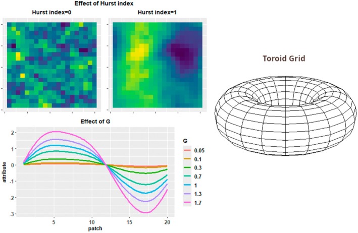 FIGURE 1
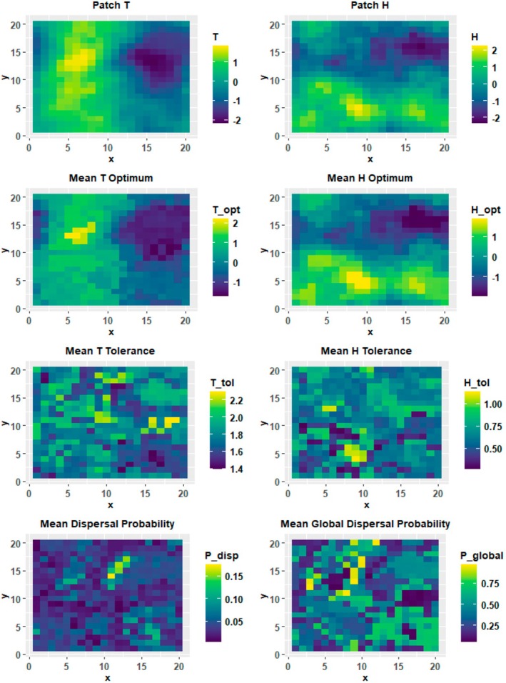 FIGURE 2
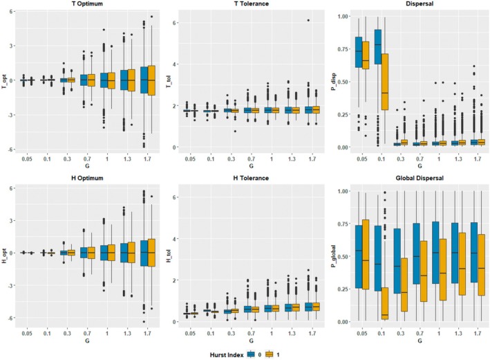 FIGURE 3
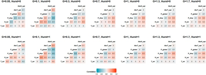 FIGURE 4
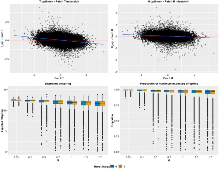 FIGURE 5
| Trait | Symbol | Distribution | Parameters |
|---|---|---|---|
| Temperature optimum | Normal |
= , = | |
| Temperature tolerance | Log‐normal | = 0, = 1 | |
| Habitat optimum | Normal |
= 0, = | |
| Habitat tolerance | Log‐normal | = 0, = 1 | |
| Dispersal chance | Uniform | 0, 1 | |
| Dispersal mode preference | Uniform | 0, 1 |
| Parameter | Symbol | Value |
|---|---|---|
| Landscape dimensions | 20 × 20 patches | |
| Total simulation time‐steps | 10,000 | |
| Niche breadth trade‐off | 3 | |
| Patch expected immigrants | 2.5 | |
| Gradient strength multiplier |
| |
| Landscape Hurst Index | Hurst |
- —Bayerisches Staatsministerium für Bildung und Kultus, Wissenschaft und Kunst10.13039/501100004563
Peer Reviews
No public reviews on file for this paper yet. If you reviewed it on a platform where reviews are public (OpenReview, ICLR, NeurIPS, ICML), you can paste yours below so the community can read it here.
Videos
No videos yet. Explain this paper in a talk, walkthrough, or lecture? Add one.
Taxonomy
TopicsEcology and Vegetation Dynamics Studies · Species Distribution and Climate Change · Animal Ecology and Behavior Studies
Introduction
1
Organisms exist within environments which vary over both time and space. Organisms can cope with spatial variation in their environments by adapting their niche optima to local conditions. Given adequate genetic variation in the population, such adaptation can occur quickly. However, successful adaptation requires organisms to cope with short‐term temporal variation in the environment (Hoffmann and Sgrò 2011). Organisms can deal with temporally variable environments by adapting their tolerances to local temporal variance. Alternatively, organisms can avoid periods of unfavorable conditions or hedge reproductive bets via dispersal (Venable and Brown 1988; Kisdi 2002), reducing the need to tolerate temporal variance in the environment (Bonte et al. 2012). However, because dispersal requires organisms to move through space and settle in new habitats, organisms relying on dispersal to avoid temporal environmental variance must be sufficiently capable of tolerating the spatial heterogeneity they encounter in their environments (Futuyma and Moreno 1988; Bonte et al. 2012). Tolerance to this spatial variation may not necessarily be conferred by tolerance to temporal variation as the environmental factors that vary over space may be different from those that vary over time. Since tolerances are critical to the ability of organisms both to stay in place and disperse, both strategies are subject to constraints (Bonte et al. 2012; Hillaert et al. 2015) imposed by trade‐offs between tolerance to environmental variation and performance under optimal conditions (Morin and Chuine 2006; Ravigné et al. 2009; Herren and Baym 2022), or trade‐offs between tolerances to variation in different environmental factors.
The evolution of local adaptation and environmental tolerances itself is affected by an organism's dispersal behavior through its effects on immigration and gene flow (Kirkpatrick and Barton 1997; Ronce and Kirkpatrick 2001; Lenormand 2002; Billiard and Lenormand 2005; Bridle et al. 2010, 2019). Dispersal and movement behavior, in turn, is informed by the risks imposed by spatial environmental heterogeneity and the selection it imposes, meaning that the evolution of local adaptation and environmental tolerances are dependent on spatial context (Bonte et al. 2006; Richardson et al. 2014; Forester et al. 2016), including the magnitude of compositional environmental heterogeneity and its spatial arrangement (Fahrig 2017). This dependence on spatial context has important implications for conservation, particularly in the face of climate change, as certain spatial structures may help or hinder local adaptation (Claudino and Campos 2014), range shifts (Burton et al. 2010; Synes et al. 2015; Årevall et al. 2018), and recolonization of habitat after disturbance (Leimar and Norberg 1997), making a thorough understanding of the effects of spatial structure on adaptation and dispersal key to creating effective conservation strategies (Holt and Barfield 2011; Årevall et al. 2018).
Studies investigating dispersal and adaptation commonly adopt a mechanistic modeling approach due to the large temporal and spatial scales such processes can occur over, the difficulty of observing them in nature, and the difficulty of experimentally manipulating conditions in the field (Hanski 2015; Ovaskainen et al. 2019). A mechanistic modeling approach has the advantage of allowing detailed experimental control over conditions while also enabling direct insight into causal mechanisms underpinning patterns by explicitly ecological and evolutionary processes (Cabral et al. 2017; Hanski 2015; Higgins et al. 2012). While numerous modeling studies have explored aspects of local adaptation (García‐Dorado 1987; Bridle et al. 2010; Claudino and Campos 2014; Kisdi et al. 2020), tolerance and niche breadth (Hillaert et al. 2015; Sieger et al. 2019; Kisdi et al. 2020), and dispersal (Hamilton and May 1977; Gros et al. 2006; Duputié and Massol 2013; Hillaert et al. 2015), few studies consider all three simultaneously. In their review of individual‐based models examining eco‐evolutionary dynamics, Romero‐Mujalli et al. (2019) found no studies which simultaneously modeled the evolution of local adaptation, dispersal, and phenotypic plasticity. Moreover, the authors also noted that studies focused on local adaptation were often not spatially explicit (e.g., Kisdi et al. 2020). Modeling studies on local adaptation which do consider spatial environmental variation tend to do so only in very simplified manners, often assuming simple linear gradients (e.g., Hillaert et al. 2015; Leidinger et al. 2021).
Meanwhile, studies modeling dispersal often explicitly consider spatial structure, but typically assume a binary habitat‐non‐habitat dichotomy (e.g., Gros et al. 2006; Claudino and Campos 2014). Such assumptions are problematic, particularly for terrestrial environments, as environmental shifts in space are often gradual, and many species exploit multiple habitat types (Hein et al. 2003; Jules and Shahani 2003), meaning it may be more appropriate in many cases to model landscapes as fractal environmental gradients or habitat mosaics (Fischer and Lindenmayer 2006; Franklin and Lindenmayer 2009). Sieger and Hovestadt (2020) used continuous fractal landscapes to explore the effect of the ratio of temporal to spatial heterogeneity on the evolution of dispersal frequency using an individual‐based model which notably modeled niche optimum, tolerance, and dispersal together as evolving traits. While the authors considered the magnitude of variation in patch environments (compositional heterogeneity), they did not explore the effects of spatial configuration despite its importance as a component of environmental spatial structure Fahrig (2017). Moreover, the authors assumed only random global dispersal and did not consider how environmental heterogeneity could affect other components of dispersal strategy such as dispersal distance, which may be affected by spatial heterogeneity independently of dispersal frequency (Gros et al. 2006; Bonte et al. 2010).
In this study, we use the model of Tardanico and Hovestadt (2023), developed as an extension of the model of Sieger and Hovestadt (2020), in order to systematically explore the effects of landscape structure on adaptation and dispersal strategy of annual asexual organisms with varying environmental niches and dispersal probabilities living, reproducing, and competing in continuous fractal landscapes. We extended the model by considering both temporally static and temporally variable patch environment attributes as well as by permitting dispersing organisms to choose between random global or nearest neighbor dispersal strategies, thus incorporating dispersal distance explicitly into the model. We specifically ask how the magnitude of spatial environmental variation, or compositional heterogeneity, and spatial environmental autocorrelation jointly affect the evolution of environmental niche optima, tolerances to environmental variation, dispersal frequency, and preference for shorter or longer distance dispersal, including the evolution of syndromes in these traits. In addition to data on organism traits such as niche optima, tolerances, and dispersal behavior, our model also records information on organism lineages and thus may be used to explore diversity patterns, which we previously explored in Tardanico and Hovestadt (2023). This study, however, will restrict itself to dealing with patterns of adaptation in organism traits.
Methods
2
We used the model which we developed for our previous study (Tardanico and Hovestadt 2023). As we made no modifications to the simulation model from our previous study, the description of the model's properties and its mechanics has been recycled from Tardanico and Hovestadt (2023).
Landscape Properties
2.1
Landscapes consist of grids of habitat patches. Patches possess two attributes one representing patch temperature (T) and second attribute (H) representing an additional, unspecified environmental variable (e.g., a soil property). Spatial distributions for the two patch attributes were generated via an R implementation of the spatially autocorrelated landscape generation algorithm from Saupe (1988). This algorithm is capable of generating fractal landscapes with varying degrees of spatial autocorrelation between grid cell values depending on the value of the Hurst index parameter. Landscapes generated with this algorithm are toroid and opposite edges connect seamlessly to each other, thereby preventing edge effects from occurring at landscape edges (Figure 1). In this study, all landscapes were generated with a Hurst index of either 0 or 1. A Hurst index of 1 produces completely spatially autocorrelated landscapes where patches always have similar environments to their immediate neighbors, while a Hurst index of 0 produces a largely random spatial distribution of patch environments (Figure 1). Spatial distributions for the two patch attributes are generated independently, meaning that T and H attributes do not necessarily correlate with each other spatially. However, T and H spatial distributions for the same landscape were generated with matching generation parameters, including the Hurst index. Thus a landscape with a highly autocorrelated spatial distribution for the T attribute will always have an equally spatially autocorrelated H attribute distribution. Values for patch environmental attributes were drawn from a normal distribution and standardized to a mean of 0 and a standard deviation of 1, such that the average frequency of different patch environment values was constant regardless of spatial configuration. Landscape dimensions were set at 20 by 20 patches for a total of 400 patches in a landscape. These dimensions were chosen in order to limit computation time while still being large enough for structure driven patterns to emerge. Landscape compositional heterogeneity, the magnitude of spatial variation in the T and H attributes, was controlled by the simulation parameter G. By multiplying patch attribute values by G, the range of patch attribute values could be expanded or reduced while maintaining a constant configuration (Figure 1). In addition to varying spatially, the T attribute fluctuates over time such that the T attribute for patches varies from one time step to the next. Fluctuations in T are global and affect all patches in a landscape equally. Fluctuations in T are normally distributed with a mean of 0 and a standard deviation of 1 and modify patch T attributes by adding the value of the fluctuation to the patch's T attribute.
Diagram of major landscape properties. Top left: Effect of Hurst index on spatial autocorrelation. Bottom left: Effect of G on magnitude of variation in patch attributes. Right: Shape of simulated world. Landscapes are toroid with interconnected edges.
Organism Properties
2.2
Patches are inhabited by populations of asexual organisms belonging to lineages which behave as a guild of ecologically similar species who compete with each other within a patch. In addition to possessing a “taxonomic” identity, lineages possess varying environmental niches and dispersal tendencies, which serve to differentiate lineages functionally from one another. Organism niches are modeled as Gaussian curves whose center and spread are defined by a niche optimum and tolerance trait, respectively. Organisms possess separate optimum and tolerance traits for T and H. T niche optimum and tolerance are represented by the T opt and T tol traits, respectively, while H optimum and tolerance represented by the H opt and H tol traits. Organisms also possess two dispersal traits, Pdisp, which defines the probability of an organism dispersing from its natal patch, and Pglobal which defines an organism's preference for one of two possible dispersal modes. Dispersal is explained further in the section below. Organism traits are summarized in Table 1. Trait values are generated when a lineage first appears in a landscape by drawing random values from statistical distributions. Niche optima are drawn from a normal distribution with a μ of 0 and σ equal to G. Tolerance traits are drawn from a log‐normal distribution with a μ and σ of 0 and 1, respectively. Dispersal traits are drawn from a uniform distribution with a minimum of 0 and a maximum of 1. Organism traits are summarized in Table 1.
Dispersal
2.3
Organisms can disperse from their natal patches to other patches. Individual organisms may disperse once during their life cycle. Whether or not an organism disperses from its natal patch is determined by drawing a random number from a uniform distribution and comparing the value with an organism's Pdisp trait. If the random number is less than or equal to the organism's Pdisp trait value, the organism will disperse. Dispersing organisms must then choose a dispersal mode. Two different modes of dispersal are possible within this model, serving as short and long distance modes. We chose to explicitly incorporate dispersal distance as a separate trait due to previous research indicating that landscape spatial structure affects dispersal distance differently from dispersal frequency (Gros et al. 2006). Organisms can disperse via nearest neighbor dispersal or random global dispersal. We chose these two dispersal methods because they are computationally lightweight, simple to implement, and already in widespread use in modeling studies (Travis and Dytham 1999; Kubisch et al. 2013, 2014; Kisdi et al. 2020). Used together, the two dispersal modes allow the model to approximate the peak and tail of a dispersal kernel without the complexity implementation and computational cost of directly simulating a dispersal kernel in a grid‐based landscape. The dispersal mode is selected by drawing a random number from a uniform distribution between 0 and 1 and comparing its value with an organism's Pglobal trait. If the number's value is less than or equal to the organism's Pglobal trait, the organism disperses via random global dispersal. If not, the organism disperses via nearest neighbor dispersal. In nearest neighbor dispersal, an organism moves to a random patch with the coordinates x + p and y + q, where x and y are the coordinates for the natal patch and p and q are integers between −1 and 1. If the target patch's coordinates are outside the bounds of the landscape, the organism is instead moved to the opposite side of the landscape due to the landscape being treated as a torus with interconnected edges, thereby avoiding the problem of artificially creating edge effects at landscape boundaries. In random global dispersal, a random patch within the landscape is selected as the target patch. In both dispersal modes, the target patch must have different coordinates from the natal patch and will be re‐selected if the target coordinates leave a dispersing organism in its natal patch.
Organism Life‐Cycle
2.4
Organisms have annual life cycles with complete replacement of the population at the end of a generation. Life cycles consist of discrete reproduction, competition, and dispersal phases. During the reproductive phase, organisms reproduce asexually to produce offspring with identical traits to their parents. The number of offspring is drawn from a Poisson distribution, with the expected reproductive output determined by an organism's fitness within its patch environment within a given time step as given by Equation (1). Here, Efert is the expected number of offspring, R0 is an organism's intrinsic maximum expected offspring (kept at a constant value of 15), Tpatch and Hpatch are the temperature and habitat values for a given patch. Reproductive output is additionally limited by a trade‐off between tolerance and maximum expected offspring, meaning that organisms with broader tolerances produce fewer offspring on average. This trade‐off serves to prevent organisms from having infinitely large tolerances. The strength of this trade‐off is determined by the trade‐off parameter α (Chaianunporn and Hovestadt 2012; Sieger et al. 2019); lower values produce stronger trade‐offs. As the effect of varying α is functionally the same as the effect of varying the strength of G, α is kept at a constant value of 3 in this study. After reproduction, offspring undergo a maturation phase in which they compete on an equal basis with other offspring within the same patch. Survival of the competition phase is density dependent and regulated via the Beverton–Holt equations (Equations 2 and 3; Beverton and Holt 1957), where SA is the expected surviving offspring, L0 is the total offspring, and K is the carrying capacity of a patch if all organisms in the patch have an Efert equal to R0 and thus perfect fitness. Note that because patch carrying capacity is affected by Efert, maladaptation may reduce the realized carrying capacity of a patch. The value of K is set at 150 individuals, which allows for relatively stable patch populations while maintaining low computation time. The number of surviving offspring are determined by drawing a random number from a binomial distribution with a mean of SA. Surviving offspring are then able to disperse to a new patch and start the cycle anew.
Immigration From External Sources
2.5
New organisms can immigrate into the landscape from the outside. The number of new immigrants is randomly drawn from a Poisson distribution with an expected value of Eimmi. In our simulations, Eimmi is set at a constant expected value of 2.5 immigrants per patch. This amounts on average to approximately 0.0011% of the expected local offspring production for a patch with a perfectly adapted population at carrying capacity. Immigrants are generated with randomized traits within a patch and added to the new generation along with existing offspring. Statistical distribution parameters for immigrant traits are summarized in Table 2.
Experiment Design
2.6
Landscapes were initialized from text files containing spatial distributions for the two patch attributes. Landscapes were initially empty with no preexisting populations and were then allowed to be colonized by immigrant organisms over the course of the simulation. Simulations were run for a total of 10,000 time steps. Simulations were run once for each landscape in a set for a total of 30 unique replicates. Fluctuations for each time step were generated at initialization. To ensure replicability, each replicate in a scenario was run with a unique, preset random number generator seed. We ran seven different compositional heterogneity scenarios (G∈0.05,0.1,0.3,0.7,1,1.3,1.7) and two spatial autocorrelation scenarios (Hurstindex∈0,1) for a total of 14 different scenarios. The simulation program recorded means and variances for trait values and fitness at each time step for entire landscapes, as well as a census of each individual organism in a landscape at the 10,000th timestep, including its lineage identity, trait values, and the patch it inhabited. The program then used the census data to calculate mean trait values and fitness for each patch in the landscape. We calculated two fitness metrics in this study, an organism's expected number of offspring, and the expected proportion of the maximum possible offspring. Model parameters used in this study are summarized in Table 2.
Data Analysis
2.7
We analyzed simulation output data in R (R Core Team 2020). Analysis was restricted to organisms belonging to lineages which had total landscape populations of 50 individuals or more at time step 10,000. We did this in order to restrict the analysis to lineages with established populations and exclude transient lineages with maladaptive trait combinations arising from the random nature of immigrant trait generation, as such lineages were unlikely to persist in the landscape beyond a few time steps. Due to the large size of the data set, we opted to sample 10,000 individuals from each scenario. In the case of the G = 1.3 scenarios, environmental fluctuations caused population crashes at the final time step, resulting in sample sizes of only 9742 (Hurst index = 0) and 9735 (Hurst index = 1) individuals, respectively. This resulted in a data set with a total of 139,477 observations. We assessed the data visually using the ggplot2 R package (Wickham 2016) and evaluated R ^2^ correlations between the six organism traits using the ggally package (Schloerke et al. 2024). We did not make use of statistical significance tests due to their lack of meaning within a mechanistic modeling context and their unreliability due to extreme sensitivity when sample sizes are extremely large (White et al. 2014).
Results
3
Organism Traits
3.1
Organism traits responded diversely to G and the Hurst index (Figures 2 and 3). Since these patterns were largely identical at the landscape level and when aggregated at the patch level, this subsection will focus on landscape level patterns. Niche optima traits Topt and Hopt matched the frequency distributions for their respective patch attributes (Figures 2 and 3), with median values close to 0 and variances which increased with increasing G. Median T tolerance (Ttol) showed little variation with G, but did increase in variance. Ttol was unaffected by the Hurst index. H tolerance (Htol) increased in both median and variance with greater G. This increase was monotonic under a Hurst index of 1, while under a Hurst index of 0 the increase was non‐monotonic between G = 0.05 and G = 0.3. Dispersal probability (Pdisp) responded non‐monotonically to increasing G, shifting from high median values and relatively large variances to very low median values with small variances across a transition zone occurring between G = 0.05 and G = 0.3. This transition zone range was affected by the Hurst index, with the transition starting earlier and declining somewhat more mildly under a Hurst index of 1. From G = 0.3 onwards, Pdisp increased slightly with greater G. Within this range, Pdisp was slightly higher under a Hurst index of 1. Global dispersal probability (Pglobal) was highly variable in nearly all scenarios and responded non‐monotonically to increasing G, initially decreasing around G = 0.1 and then rebounding thereafter. This pattern was notably stronger under a Hurst index of 1. Median Pglobal was consistently higher under a Hurst index of 0 (Figure 3).
Example spatial maps of patch attributes and patch mean trait values for a single simulation replicate (G = 1, Hurst index = 1).
Box plot of distributions for organism trait values by G and Hurst index scenario at time step 10,000. N = 9742 (G = 1.3, Hurst index = 0), N = 9735 (G = 1.3, Hurst index = 1), N = 10,000 (all other scenarios).
Relationships Between Organism Traits
3.2
Compositional heterogeneity and spatial autocorrelation affected the correlational relationships between organism traits (Figure 4). Compositional heterogeneity had the strongest effect on correlations between traits; spatial autocorrelation tended to mediate the strength of those correlations. In scenarios with a Hurst index of 1, trait correlations tended to be slightly stronger, although this effect was not universal.
R 2 correlations between trait values by G and Hurst index scenario for individual organisms. Niche optima are absolute value transformed. N = 9742 (G = 1.3, Hurst index = 0), N = 9735 (G = 1.3, Hurst index = 1), N = 10,000 (all other scenarios).
Trait correlations shifted between three distinct patterns as G increased. The first pattern occurred at G = 0.05 and was characterized by strong but dramatically inconsistent relationships between traits. At G = 0.1, this pattern gave way to a pattern characterized by negative correlations between absolute value niche optima (T opt and H opt), P disp and positive correlations between P disp, P global, and H tol. A negative correlation between P global and absolute value niche optima traits occurred under a Hurst index of 1 under this pattern, but not under a Hurst index of 0. Further increases in G resulted in a shift to a third pattern characterized by positive associations between absolute value niche optima, P disp, and H tol, and negative associations between P disp and P global, and between P global and absolute value H opt. Additionally, under a Hurst index of 1 there was a slight but consistent negative relationship between P global and H tol while the relationship between P disp and P global was slightly stronger. Associations were typically stronger with absolute value H opt than T opt.
T tol exhibited weak and inconsistent correlations with other traits across all scenarios, with a slightly higher tendency toward weak positive correlations with absolute value niche optima traits in Hurst index = 0 scenarios at or above G = 0.3. Correlations with T tol tended to be strongest overall below G = 0.3; in G = 0.1 and G = 0.05 scenarios, T tol had a consistent negative correlation with P disp.
Adaptation and Fitness
3.3
Organisms were overall well adapted to their local patch conditions, with niche optima closely correlating with patch environment attributes. This correlation was strongest for H opt, with T opt tending to be more variable in relation to patch T (Figure 5). Species inhabiting more extreme patches had a tendency toward greater mismatches between niche optima and patch attributes; this pattern was stronger for the T attribute than the H attribute.
Individual local adaptation and fitness as measured by fertility. Top: Difference between individual niche optima and respective patch attributes versus patch attribute. Bottom: Box plots of distributions at time step 10,000 by scenario of individual expected offspring and the proportion of maximum expected offspring, the expected number of offspring under optimal conditions. N = 9742 (G = 1.3, Hurst index = 0), N = 9735 (G = 1.3, Hurst index = 1), N = 10,000 (all other scenarios).
Accordingly, fitness was relatively high, with the vast majority of organisms having at over 80% of their maximum fertility without accounting for reduced fertility due to the tolerance trade‐off. Factoring in the tolerance trade‐off, most individuals had expected at least 75% of their maximum fertility (Figure 3). Fertility declined slightly and increased in variance with increasing G.
Discussion
4
Landscape spatial structure affected niche traits and local adaptation, dispersal traits, and correlational relationships between traits. Patterns were most strongly influenced by compositional heterogeneity (G), with spatial autocorrelation (Hurst index) mostly playing a mediating role. Dispersal traits were an exception to this and were notably affected by both compositional heterogeneity and spatial autocorrelation. Niche optima distributions reflected the distributions of patch environment attributes in the landscapes and organisms were typically well adapted to their local patches, in line with theoretical studies findings that greater spatial heterogeneity selects for local adaptation due to the risk imposed by the landscape of immigrating into an unsuitable habitat (Hastings 1983; Futuyma and Moreno 1988). Tolerance traits behaved differently for the two environmental attributes. T tolerance was notably higher than habitat tolerance and was weakly affected by landscape structure, resembling the results of Sieger and Hovestadt (2020), and lacked any consistent relationships with other traits under most scenarios. H tolerance, on the other hand, showed a clear relationship with landscape structure at both the patch and landscape level. The difference in behavior of the two tolerance traits indicates that tolerance is determined primarily by the degree to which environmental variation can be avoided. In this model, and for many climate related environmental variables, temporal fluctuations are both unpredictable and can occur synchronously over a large area and thus affect organisms independently of spatial context or dispersal capabilities. Such environmental variation selects for broad niches that permit consistent fitness over a large range of conditions (Lynch and Gabriel 1987; Futuyma and Moreno 1988; Devictor et al. 2008; Lin and Wiens 2017), potentially overriding effects of smaller scale spatial variation. Purely spatial environmental variation, on the other hand, can be avoided substantially by restricting movement and dispersal, allowing organisms to retain more specialized niches.
Dispersal trait responses to compositional heterogeneity and spatial autocorrelation were nonlinear in nature and were largely consistent with established literature regarding relationships between dispersal frequency, dispersal distance, and spatial heterogeneity (Burgess et al. 2016). Dispersal shifted from a pattern of high dispersal probabilities at low levels of compositional heterogeneity to very low dispersal probabilities once heterogeneity increased beyond a threshold range, with slight increases in dispersal occurring at very high levels of compositional heterogeneity. Global dispersal probability shifted from a maximum at very low compositional heterogeneity to a minimum around the threshold range at which dispersal probability shifted and rebounded thereafter. Frequent dispersal is expected under very low spatial heterogeneity because there is little spatial variation in fitness and thus little risk to dispersal, while kin competition imposes a positive selection on dispersal (Hamilton and May 1977; Nakajima and Kurihara 1994; Gandon 1999). Moreover, kin competition selects for longer dispersal distances as this allows organisms to minimize the chance of encountering kin in a destination patch (Hovestadt et al. 2001; Rousset and Gandon 2002), resulting in a preference for random global dispersal under very low heterogeneity. Increasing compositional heterogeneity beyond a certain threshold resulted in a decline in dispersal chance across a transition zone as compositional heterogeneity began to exceed the limits of tolerances and impose increasingly significant fitness costs to dispersal (Hastings 1983; Holt 1985). This threshold itself was dependent on spatial autocorrelation and selection on dispersal traits within the transition zone was strongly divergent between autocorrelation scenarios. In the G = 0.1 scenarios, high autocorrelation produced an extremely broad range of dispersal probabilities and the lowest global dispersal probabilities of any scenario, while dispersal trait distributions under low autocorrelation were similar to other low heterogeneity scenarios. The discrepancy between the two autocorrelation scenarios when G = 0.1 is the result of several factors. Under low autocorrelation, unpredictable spatial variation selects for higher H tolerance, reducing risks associated with dispersal and making organisms less sensitive to spatial variance in the environment. In contrast, the predictability of spatial variation in highly autocorrelated landscapes results in lower H tolerance and thus greater sensitivity to spatial context. As a consequence, dispersal in the high autocorrelation G = 0.1 scenarios is subject to a range of different selective pressures depending on an organism's environmental niche. Organisms adapted to common habitats, or those with broad tolerances face relatively low dispersal risks as suitable habitat is plentiful, while organisms with more narrow niches, or those adapted to rarer or more extreme environments face high risks when dispersing resulting in selective pressure toward lower dispersal probabilities. The predictability of spatial variation in high autocorrelation scenarios also strongly favors nearest neighbor dispersal over random global dispersal if dispersal is undirected, as it will almost always result in an organism landing in a suitable patch under moderate compositional heterogeneity, while random global dispersal carries significant risk of emigration into an unsuitable patch (Bonte et al. 2010). In the absence of spatial autocorrelation, there is no meaningful advantage to either dispersal method, causing global dispersal to behave as a largely neutral trait. At G = 0.3 and above, spatial heterogeneity strongly selects for low dispersal probabilities; dispersal probabilities in these scenarios were similar to those observed by Sieger and Hovestadt (2020). Increases in dispersal and global dispersal probabilities with further increases in G above 0.3 indicate increasing selection for bet‐hedging against temporal heterogeneity due to decreasing habitat area. Dispersal was slightly but consistently higher in highly autocorrelated scenarios at and above G = 0.3 while global dispersal probability was consistently lower. These findings are consistent with the results of Hovestadt et al. (2001), which also found that higher spatial autocorrelation favored increased local dispersal propensity and distance and disfavored global dispersal.
Patterns of correlation between traits responded in a nonlinear fashion, with abrupt shifts in patterns at two thresholds of compositional heterogeneity, one above G = 0.1 and another threshold below G = 0.1. Above G = 0.1, patterns were highly similar between scenarios, with absolute value niche optima showing consistent positive relationships with tolerances and dispersal chance, and a consistent negative relationship between dispersal chance and global dispersal that diminishes with greater heterogeneity. Meanwhile, patterns at G = 0.1 were characterized by positive associations between dispersal chance, global dispersal, and H tolerance, and negative associations between H tolerance and dispersal traits, and absolute value niche optima. These results mirror those of Sieger and Hovestadt (2020), which found a shift in the location of the most frequent dispersers from the most common habitats to rare patches with more extreme environments as spatial heterogeneity increased, driven by greater selection for bet‐hedging strategies in organisms living in extreme patches. Similarly, trait correlation patterns in our model above G = 0.1 are consistent with increasingly strong selection for bet‐hedging strategies as niche optima move further away from average landscape conditions. This is further supported by a pattern of lower fitness in organisms adapted to more extreme conditions and the tendency for such organisms to be adapted to slightly more average conditions than those they experienced in their habitat patches. These patterns appear to be consequences of the smaller habitat area available to organisms with more extreme niche optima. The small habitat area reduces the population sizes that can be supported and renders such organisms particularly vulnerable to temporal environmental fluctuations (Lande 1993; Hanski 1998; Hill and Caswell 1999), increasing the importance of risk spreading strategies for population persistence. The need for insurance against temporal fluctuations may partly explain the slight tendency of “regression toward the mean” (Sieger and Hovestadt 2020) for niche optima in extreme patches as this apparent maladaptation may potentially expand the number of patches an organism can survive in at any given time. Below G = 0.1, trait correlations became highly idiosyncratic and inconsistent. This is likely due to a combination of very low variance in niche traits, weak selection within the range of values they occupy, very weak selection on dispersal traits, and highly uneven landscape communities dominated by a small number of lineages, leading to correlational patterns which are highly influenced by stochasticity and priority effects.
This model makes a number of simplifying assumptions for ease of implementation, computation, and analysis which, if altered, could affect selection on traits and resulting trait patterns. Our model assumes that organisms are asexual with an annual life cycle with no overlapping generations and does not consider other life histories or reproductive strategies. Longer lifespans allow for multiple bouts of reproduction which can serve to hedge reproductive bets in the face of temporal by spreading reproduction out over time (Danforth 1999; Hopper 1999; Gremer and Venable 2014). Inclusion of competing annual semelparous organisms and perennial iteroparous organisms would likely produce a pattern of succession over the course of the simulation with annual organisms dominating in the early stages and being gradually replaced by perennial organisms as the simulation progresses. Longer lifespans may also have the effect of reducing population turnover resulting in slower shifts in community level trait patterns. Inclusion of overlapping generations, meanwhile, has the potential to alter selection on dispersal traits as a result of the effect of age structure on kinship competition (Ronce et al. 2000). Including dormancy would provide organisms, including organisms with annual, semelparous life cycles, with an alternative means of hedging against reproductive risk by serving as a kind of dispersal through time (Buoro and Carlson 2014). As dormancy and dispersal serve similar bet hedging functions, the addition of dormancy as a possible strategy would likely reduce dispersal frequency. Organisms in our model are limited to two dispersal modes, and dispersal is assumed to be both undirected and unaffected by an organism's local environment or fitness. Undirected, uninformed dispersal can incur a notable fitness cost due to the risk that an organism will emigrate to an unsuitable patch or at an inopportune time (Hastings 1983; Bonte et al. 2010), necessitating greater tolerance which comes at the cost of maximum expected reproductive output in this model. Informed and directed dispersal can greatly reduce dispersal risk related fitness costs, particularly for long distance dispersal and under strong or unpredictable spatial environmental variation (Lakovic et al. 2015; Sieger and Hovestadt 2021). Reducing these fitness costs would likely permit more frequent dispersal and a higher reproductive output due to reduced selection for high tolerance. Finally, interactions with other organisms could affect selective pressures on traits in a variety of complex ways (Chaianunporn and Hovestadt 2012, 2019), but this model only considers competition.
Conclusions
5
Our study systematically explored the role of compositional heterogeneity and spatial autocorrelation in shaping both adaptation to environmental conditions and dispersal behavior in a temporally variable environment, something which to our knowledge has not been systematically explored by previous studies. Our model reproduced a number of patterns observed in previous theoretical studies stemming from varying degrees of selective pressure imposed by the spatial and temporal environments. We found that niche adaptation and dispersal patterns were primarily driven by a balance between pressure to avoid risk imposed by spatial heterogeneity and pressure to hedge against risk imposed by large‐scale temporal environmental fluctuations. Compositional heterogeneity tended to have the strongest influence over patterns while spatial autocorrelation typically played a mediating role. We found that dispersal frequency and dispersal distance were affected differently by spatial structure, underscoring the need to consider the two independently. Future studies should explore alternative life‐history and dispersal scenarios, as well as explore how a shifting environment interacts with landscape spatial structure to influence patterns of adaptation and dispersal behavior.
Author Contributions
Joseph Tardanico: conceptualization (equal), formal analysis (equal), investigation (lead), methodology (lead), visualization (lead), writing – original draft (lead). Thomas Hovestadt: conceptualization (equal), formal analysis (equal), funding acquisition (lead), writing – review and editing (lead).
Conflicts of Interest
The authors declare no conflicts of interest.
Supporting information
Figures S1–S5
The reference list from the paper itself. Each links out to its DOI / PubMed record.
- 1Årevall, J. , R. Early , A. Estrada , U. Wennergren , and A. C. Eklöf . 2018. “Conditions for Successful Range Shifts Under Climate Change: The Role of Species Dispersal and Landscape Configuration.” Diversity and Distributions 24, no. 11: 1598–1611.
- 2Beverton, R. J. H. , and S. J. Holt . 1957. On the Dynamics of Exploited Fish Populations. Fishery Investigations Series II Volume XIX, Ministry of Agriculture, Fisheries and Food. Springer Dordrecht. 10.1007/978-94-011-2106-4. · doi ↗
- 3Billiard, S. , and T. Lenormand . 2005. “Evolution of Migration Under Kin Selection and Local Adaptation.” Evolution 59, no. 1: 13–23.15792223 · pubmed ↗
- 4Bonte, D. , J. V. Borre , L. Lens , and J.‐P. Maelfait . 2006. “Geographical Variation in Wolf Spider Dispersal Behaviour Is Related to Landscape Structure.” Animal Behaviour 72, no. 3: 655–662.
- 5Bonte, D. , T. Hovestadt , and H.‐J. Poethke . 2010. “Evolution of Dispersal Polymorphism and Local Adaptation of Dispersal Distance in Spatially Structured Landscapes.” Oikos 119, no. 3: 560–566.
- 6Bonte, D. , H. Van Dyck , J. M. Bullock , et al. 2012. “Costs of Dispersal.” Biological Reviews 87, no. 2: 290–312.21929715 10.1111/j.1469-185X.2011.00201.x · doi ↗ · pubmed ↗
- 7Bridle, J. R. , M. Kawata , and R. K. Butlin . 2019. “Local Adaptation Stops Where Ecological Gradients Steepen or Are Interrupted.” Evolutionary Applications 12, no. 7: 1449–1462.31417626 10.1111/eva.12789 PMC 6691213 · doi ↗ · pubmed ↗
- 8Bridle, J. R. , J. Polechová , M. Kawata , and R. K. Butlin . 2010. “Why Is Adaptation Prevented at Ecological Margins? New Insights From Individual‐Based Simulations.” Ecology Letters 13, no. 4: 485–494.20455923 10.1111/j.1461-0248.2010.01442.x · doi ↗ · pubmed ↗