Fixed point-based stability analysis of climate and Langevin models
Syed Khayyam Shah, Waleed Eltayeb Ahmed, Ishraq Alabdi, Ayman Alahmade, Khaled Aldwoah, Eltigani I. Hassan

TL;DR
This paper explores how fixed point theory can help analyze the stability of climate and Langevin models.
Contribution
The paper introduces fixed point-based methods to assess stability and consistency in climate and Langevin models.
Findings
Fixed point theory is applied to prove the existence and uniqueness of solutions in climate models.
Various contraction types are reviewed for their relevance to model stability.
Theoretical foundations are linked to practical applications in model analysis.
Abstract
In this manuscript, the existence and uniqueness of solutions to equations associated with climate change are discussed. For this purpose, we utilize some results from the existing literature to investigate the behavior of these equations. Additionally, the role of fixed point theory in emphasizing the importance of proving the stability and consistency of the models is explored. Several definitions and results, such as the F-contraction, α-F-contraction, rational type (ψ,ϕ)-contraction, and Geraghty type contraction, are recalled from the existing literature to illustrate their theoretical foundations and practical applications.
Genes, proteins, chemicals, diseases, species, mutations and cell lines named across the full text — each resolved to its canonical identifier and authoritative record.
Click any figure to enlarge with its caption.
 Figure 1
 Figure 2
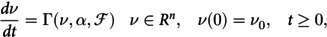 Figure 3
 Figure 4
 Figure 5
 Figure 6
 Figure 7
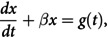 Figure 8
 Figure 9
 Figure 10
 Figure 11
 Figure 12
 Figure 13
 Figure 14
 Figure 15
 Figure 16
 Figure 17
 Figure 18
 Figure 19
 Figure 20
 Figure 21
 Figure 22
 Figure 23
 Figure 24
 Figure 25
 Figure 26
 Figure 27
 Figure 28
 Figure 29
 Figure 30
 Figure 31
 Figure 32
 Figure 33
 Figure 34
 Figure 35
 Figure 36
 Figure 37
 Figure 38
 Figure 39
 Figure 40
 Figure 41
 Figure 42
 Figure 43
 Figure 44
 Figure 45
 Figure 46
 Figure 47
 Figure 48
 Figure 49
 Figure 50
Peer Reviews
No public reviews on file for this paper yet. If you reviewed it on a platform where reviews are public (OpenReview, ICLR, NeurIPS, ICML), you can paste yours below so the community can read it here.
Videos
No videos yet. Explain this paper in a talk, walkthrough, or lecture? Add one.
Taxonomy
TopicsNonlinear Differential Equations Analysis · Fixed Point Theorems Analysis · Numerical methods for differential equations
1 Introduction
Mathematics serves as a highly efficient and potent tool for understanding the world and addressing intricate challenges across diverse scientific fields, engineering, and technology [1–3]. In this context, the crucial role of mathematics cannot be overstated in addressing planetary issues, particularly the connection between society and nature [4,5]. Humans engage in various activities through interactions with their environment. Humans influence the environment by altering its properties, while environmental conditions, in turn, impact human health and survival capabilities. The present climate change, in contrast to other instances, is anthropogenic and marked by an unparalleled acceleration in the global mean surface temperature (GMST) [6,7]. In [8], it is indicated that from 1880, the GMST has risen upto 0.07 C by an average per decade. In the 21st century, notably in the first two decades, the growth rate of the GMST was 0.17 C for a decade, which is more than twice the average rate. A notable indicator of human activities is the considerable rise in atmospheric carbon dioxide (CO_2_) concentrations. This greenhouse gas, a by-product of the combustion of fuels, turns out to be the primary culprit for global warming. This greenhouse gas, a by-product of fuel combustion, is considered the primary driver of global warming.
Global warming has impacted climate across nearly all regions of our planet; however, the extent of this effect varies considerably by region [6,7]. Global and regional climate changes evidently influence individuals and their activities [9,10]. Evaluating climate hazards is a necessary step in determining how humanity may be affected by changing climate conditions [11]. Mathematics and its methodologies are essential in climate study [12,13]. It can be asserted assuredly that mathematics is the sole discipline that enables us to measure and forecast the impacts of external natural and man-made disturbances on the dynamics of the climate system. Quantitative research fundamentally relies on mathematical representations of the systems and objects being studied. In this context, we see that replicating climate and forecasting its alterations due to external influences, unlike traditional physics problems, possesses a fundamental characteristic stemming from the inability to conduct comprehensive direct physical experiments. This highlights the importance of stability of the solutions of the equations associated with climate change models is of great importance.
The equation,
denotes the mathematical representation of the Earth’s Climate System (ECS) [14–16], encompassing its dynamic development. Here, is a vector of state variables that delineate the system’s state at time t, while represents its initial state. The parameter vector governs the complex traits of the system, and symbolizes external forcing, such as solar radiation or anthropogenic impacts. This system of three-dimensional nonlinear partial differential equations captures the intended connection between internal climate parameters and external influences, offering a deterministic, semi-dynamic formulation.
The Langevin equation draws the interest of researchers, as it possesses significant importance in stochastic dynamics. This equation is commonly utilized to demonstrate the systems affected by deterministic forces and random fluctuations [14]:
where x represents the state variable, stands for the damping effect with g(t) means the external influence on the system.
Fixed point theory (FPT) is significant for analyzing mathematical models that represent climate change. FPT provides the groundwork for showcasing the stability and consistency of solutions for differential and integral equations associated with these models. In the models of Climate proper simulation, good mathematical modeling is essential for stability and predictability, notably with the help of fixed-point results like Banach’s Fixed Point Theorem, etc. This indicates that, at a fixed point, we may determine if a stable solution exists to which this system will converge under particular conditions. These methods ensure the existence and stability of solutions, which is essential for analysis and informed decision-making.
In this direction, this manuscript examines the worth of the FPT in investigating the stability of those equations that are in association with the climate change system. In this direction, some important contractions such as F-contraction, -F-contraction, rational type -contraction, and Geraghty type contraction have been recalled and utilized to define the existence and uniqueness criteria for those equations. The objective is to emphasize the fundamental characteristics that guarantee the practical effectiveness of these models in the disciplines of meteorology and climatology by conducting a thorough analysis and applying fixed-point theorems from the existing literature.
2 Preliminaries
Onward, we will denote the fixed point as (FP) and the unique solution as (Uni-Sol).
Some important definitions in this sequel are listed below:
Definition 2.1. [17] For a non-empty set , define with , if the below hold:
. . , .
Then, we labeled as -metric space.
Definition 2.2. [18] Suppose represent a mapping which fulfill the below conditions:
(1) is strictly increasing, i.e., when , for all implies to ϝ ( σ ) < ϝ ( ∋ ) .(2) For each sequence of positive terms, iff .(3) There is in a sense that .
Example 2.1. [19] For :
, , , ,
are all the examples of .
Definition 2.3. [3] Let represent a -metric space, and let be a sequence in with . Then the sequence is referred to be:
(a) convergent in and converges to e when, for every , there exists in a way that for all n>n0, and will be expressed as or as .
(b) Cauchy if, for every , there is some such that for all .
Definition 2.4. [3] Let denote a -metric space then, it is labeled as complete if every Cauchy Sequence in converges.
Definition 2.5. [19] For a non-empty set , a mapping will be -admissible when there exists a function in a sense
Definition 2.6. [20] Suppose express the structure metric space, a mapping will be termed Ćirić type generalized -contraction when there is in a sense that,
while
Theorem 2.1. [20] Suppose represent a complete metric space and is a Ćirić type generalized . When B or is continuous, then B admits a unique FP.
Definition 2.7. [19] Suppose express a metric space, a mapping be labeled as modified -contraction. When for functions and some exists such a way that and,
where
Theorem 2.2. [19] Suppose express a complete metric space, when a continuous mapping is contraction and , with . Then B possesses a unique FP.
Definition 2.8. [21] Suppose a family of functions , as with the property of:
Theorem 2.3. [21] Suppose represent a complete metric space. Suppose be a self-map fulfilling the below:
where . So this will ensure a unique FP for C.
Definition 2.9. [22] For b-metric space with , suppose is a set representing all the functions that are defined as that satisfy the below
Theorem 2.4. [22] Suppose represents a complete b-metric space along . Moreover, let denotes a self-map. If there exists in a sense that
where
then ensures a unique FP.
Consider the following two functions,
a monotone non-decreasing and continuous function with iff
is a lower semi-continuous function in a way that iff
Theorem 2.5. [23] Suppose represent a complete metric space and suppose represent a mapping. Let
whereas
Then there will be a unique point in a sense that .
3 Existence results for ECS’s equation
In this section, various important contractions from the fixed point theory will be utilized to investigate the stability of the equation associated with ECS.
where represents the vector of state variables that define the system’s state at certain points in time t, represents a specified initial condition of a system, n denotes the dimension for a dynamical system, express the m-dimensional parameter vector along representing external forcing. By transforming the differential equation into the integral form, the model equation will become:
In this direction, we aim to establish an existence result for investigating the solution of the integral equation of the type (7), utilizing Definition 2.6 and Theorem 2.1 from the existing literature.
Now, our objective is to demonstrate the existence of a solution to the integral Eq (7) in the given space and also to verify the uniqueness of the solution.
Let denote the set of all real-valued continuous functions defined on . We define as follows:
Evidently, represent a complete metric space.
Here is our first new result.
Theorem 3.1. Suppose the following presumptions are fulfilled:
(b) The function is continuous on with , and , correspondingly.(c) and for every ,
where is defined in Definition 2.6.
Then, (7) will have a Uni-Sol.
Proof: Define a map
The existence of a FP of in (9) will be evidently the Uni-Sol of the Eq (7).
Now utilizing (8) and the above presumptions (b) to (c).
This means that
Define by
Implies that,
Thus, all the assumptions of Theorem 2.1 are true. Hence, the Eq (7) will have a Uni-Sol.
For our next new result let represent all the real valued continuous functions on .
Let us define as follows
Evidently, represent a complete metric space.
Theorem 3.2. Suppose the following presumptions are fulfilled:
(r) The function is continuous on with , and , correspondingly.(s) and for every ,
where is defined in Definition 2.7.
Then, (7) will have a Uni-Sol.
Proof: Define a map
The existence of a FP of in (11) will be evidently the Uni-Sol of the Eq (7).
Now utilizing (11) and the above presumptions (r) to (s),
As a result,
Define by
Next define by
Accordingly,
Thus, all the presumptions of Theorem 2.2 hold true. So, the equation (7) will have a Uni-Sol.
Following the same flow, taking important results of Geraghty-type contractions in the framework of b-metric space, we can have novel existence and uniqueness results.
Let represent all the real valued continuous functions on .
Let us define as follows
Evidently, is a complete b-metric space with .
Theorem 3.3. Suppose the following presumptions are fulfilled:
(e) The function is continuous on with , and , correspondingly.(f) and for every ,
where is defined in Theorem 2.4.
Then, (7) will have a Uni-Sol.
Proof: Define a map
The existence of a FP of in (13) will be evidently the Uni-Sol of the Eq (7).
Now, utilizing (12), (13) and the above presumptions (e) and (f)
Further, since
It implies that,
Define by
Thus, ( 14 ) becomes,
Thus, all the necessities of Theorem 2.4 are true. So, the Eq (7) will have a Uni-Sol.
Let us define as follows
Evidently, represent a complete metric space.
Theorem 3.4. Suppose the following presumptions are fulfilled:
(m) The function is continuous on , , and , correspondingly.(n) For all and for all ,
where and are defined in Theorem 2.5.
Then, (7) will have a Uni-Sol.
Proof: Define a map
The existence of a FP of in (16) will ensure a Uni-Sol of the integral Eq (7).
Now, utilizing (15) and the above presumptions (m) and (n),
Further,
Hence,
Define by
Thus, all the necessities of Theorem 2.5 hold true. So, the Eq (7) will have a Uni-Sol.
Example 3.1. Consider the climate model described by the integral equation
where represents the temperature anomaly, is the climate feedback parameter, models external forcing, and is the initial condition.
Let represent set of all real-valued functions with no discontinuity on [0,T], endowed with the metric
Define the operator by
To verify the conditions of Theorem 3.1, note that for all ,
Using the inequality , it follows that
Let and define . Then,
which satisfies the Ćirić-type contraction condition.
Moreover, the function
is continuous in both and t.
Additionally, the growth condition
holds with M(u,y) = dm(u,y), since for .
Therefore, all the conditions of Theorem 3.1 are true, and thus integral equation admits a unique solution .
4 Existence results for Langevin equation
In this section, the same approach is utilized to investigate the stability of the Langevin equation.
where, g(t) is the external force, is a positive constant (damping coefficient or stabilizing term).
Using the technique of green function, the Eq (17) can be transformed to
where the Green function that describes how the system responds to the external forcing is
Let represent set of all real-valued functions with no discontinuity. Let us define as
Evidently, represents a complete -space.
Theorem 4.1. Assume the fulfillment of the following hypotheses:
(a2) The function is continuous on , , and , correspondingly.(a3) ,
(a4) ,
Where M(s,t) is defined in Definition 2.6 and .
Then the Eq (18) will have a unique solution.
Proof: Define a map
The existence of a FP of B in ( 20 ) will guarantee a Uni-Sol of the integral Eq ( 18 ).
Now utilizing (20) and the above presumptions (a2) to (a3),
This means that
Define by
Implies that,
Thus, all the necessities of Theorem 2.1 hold true. So, the Eq (18) will have a Uni-Sol.
Theorem 4.2. Consider that the subsequent assumptions are met:
(b2) The function is continuous on , , and , correspondingly.(b3) ,
(b4) ,
where Ma(s,t) is defined in Definition 2.7.
Then, ( 18 ) will have a Uni-Sol.
Proof: Define a map
The existence of a FP of B in ( 21 ) ensures a Uni-Sol of the integral Eq ( 18 ).
Now utilizing (21) and the above presumptions (b2) to (b3),
Hence,
Define by
Therefore,
Next define by
It implies that,
Thus, all the necessities of Theorem 2.2 hold true. Hence, the Eq (18) will have a Uni-Sol.
Let represent set of all real-valued functions with no discontinuity and define as
Evidently, is a complete b-metric space.
Theorem 4.3. Assume the below presumptions fulfill:
(c1) The function defined to be continuous on , , and , correspondingly.(c2) For all
(c3) ,
where is defined in Theorem 2.4.
Then, (18) will have a Uni-Sol and consequently will be stable.
Proof: Define a map
The existence of a FP of B in ( 23 ) ensure a Uni-Sol of the integral Eq ( 18 ).
Now, utilizing (22) and the above presumptions (c1) to (c3)
Further, since ,
Accordingly,
Define by
Thus, ( 24 ) becomes,
Thus, all the necessities of Theorem 2.2 are true. So, the Eq (18) will have a Uni-Sol and consequently will be stable.
Let represent set of all real-valued functions with no discontinuity and define as
Evidently, represent a complete metric space.
Theorem 4.4. Assume the fulfillment of the following hypotheses:
(m1) The function is continuous on , , and , correspondingly.(m2) For all
(m3) ,
Then, ( 18 ) will have a Uni-Sol.
Proof: Define a map by
The existence of a Uni-Sol of the integral Eq ( 18 ) is equivalent to the existence of a FP of B in ( 26 ).
Now, utilizing (26), (25) and the above presumptions (m1) - (m2)
Further,
Hence,
Define by
Therefore, all the necessities of Theorem 2.5 hold true. So, the Eq (18) will have a Uni-Sol and consequently will be stable.
Example 4.1. Let the integral equation:
where the Green’s function K(t,s) for is defined as
Let , and . Then the equation becomes:
Define , the space of real-valued functions with no discontinuity on [0,T], endowed with the metric:
Define the operator by
For all ,
where M(s,t) is defined in Theorem 4.1 and we may take .
for , so the kernel satisfies the integral growth condition.
All conditions of Theorem 4.1 turn true. Therefore, the equation admits a unique solution .
5 Conclusion
This paper investigates the stability of some climate systems models. In this direction, some important contractions such as F-contraction, -F-contraction, rational type -contraction, and Geraghty type contraction have been utilized to formulate some novel existence results to ensure the stability of these models. The objective is to emphasize the fundamental characteristics that guarantee the practical effectiveness of these models in the disciplines of Meteorology and Climatology by conducting thorough analysis and applying fixed-point theorems from the existing literature. The uniqueness and existence of these models are significant for making sure that the models are accurate and reliable, which in turn is necessary for making smart decisions about climate change and disasters.
The reference list from the paper itself. Each links out to its DOI / PubMed record.
- 1Stroud K. Essential mathematics for science and technology: a self-learning guide. South Norwalk, CT, USA: Industrial Press; 2009.
- 2Riley KF, Hobson MP. Student solution manual for mathematical methods for physics and engineering. 3rd ed. Cambridge, UK: Cambridge University Press; 2019.
- 3Aldwoah K, Shah SK, Hussain S, Almalahi MA, Arko YAS, Hleili M. Investigating fractal fractional PD Es, electric circuits, and integral inclusions via (ψ,ϕ)-rational type contractions. Sci Rep. 2024;14(1):23546. doi: 10.1038/s 41598-024-74046-8 39384570 PMC 11464774 · doi ↗ · pubmed ↗
- 4Yang X-S. Introductory mathematics for earth scientists. Edinburgh, UK: Dunedin Academic Press; 2009.
- 5Brocker J, Calderhead B, Cheraghi D, Cotter C, Holm D, Kuna T, et al. Mathematics of planet earth. London, UK: World Scientific Publishing; 2017.
- 6Stocker TF, Qin D, Plattner GK, Tignor M, Allen SK, Boschung J, et al. Contribution of working group I to the Fifth assessment report of the intergovernmental panel on climate change. Climate change 2013: the physical science basis. Cambridge, UK, New York, NY, USA: Cambridge University Press; 2013.
- 7Masson-Delmotte V, Zhai P, Pirani A, Connors SL, Pean C, Berger S, et al. Summary for policymakers. Climate change 2021: the physical science basis. Cambridge, UK: Cambridge University Press; 2021.
- 8Soldatenko S, Yusupov R, Colman R. Cybernetic approach to problem of interaction between nature and human society in the context of unprecedented climate change. SPIIRAS Proc. 2020;19:5–42.