Kinetic Monte Carlo Modeling of the Spontaneous Deposition of Platinum on Au(111) Surfaces
María Cecilia Gimenez, Oscar A. Oviedo, Ezequiel P. M. Leiva

TL;DR
This paper uses simulations to study how platinum atoms spontaneously deposit on gold surfaces, revealing how island structures form and grow.
Contribution
The study is the first to extensively analyze the relationship between island size, density, and spontaneous deposition.
Findings
Pt deposition on Au(111) surfaces forms ramified 2D islands up to a coverage of θ=0.25.
The mean island size and density depend strongly on the deposition rate.
The results align with experimental observations of island morphology.
Abstract
The spontaneous deposition of platinum (Pt) atoms on Au(111) surfaces is systematically investigated through kinetic Monte Carlo simulations within the Embedded Atom Model framework. The kinetic model aims to capture both stoichiometric, atomic-scale interactions and the more relevant processes that describe the kinetics of a physical problem. Various deposition rates are examined, encompassing a thorough exploration of Pt adsorption up to a coverage degree of θ=0.25. The resulting 2D islands exhibit a ramified structure, mirroring the experimental methodologies. For the first time, this study extensively analyzes the dependence of both the mean island size and island density on spontaneous deposition, thereby offering valuable insights into the intricate dynamics of the system.
Genes, proteins, chemicals, diseases, species, mutations and cell lines named across the full text — each resolved to its canonical identifier and authoritative record.
Click any figure to enlarge with its caption.
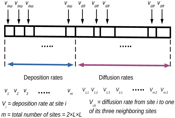 Figure 1
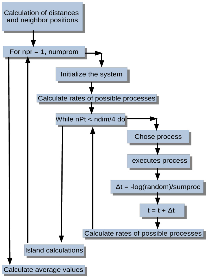 Figure 2
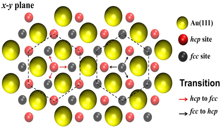 Figure 3
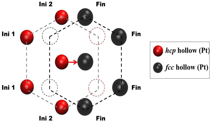 Figure 4
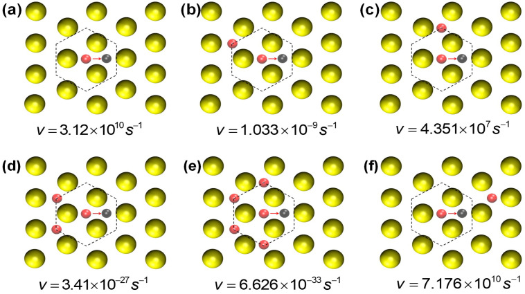 Figure 5
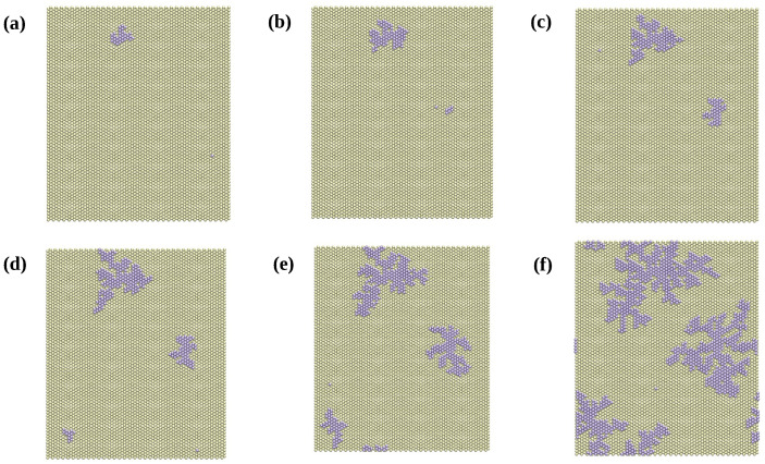 Figure 6
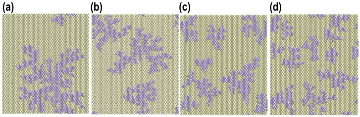 Figure 7
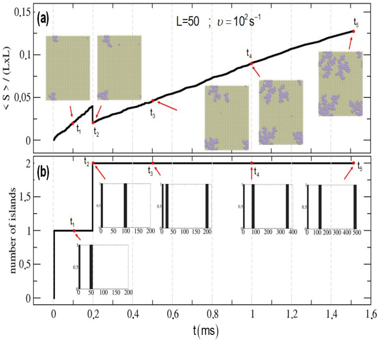 Figure 8
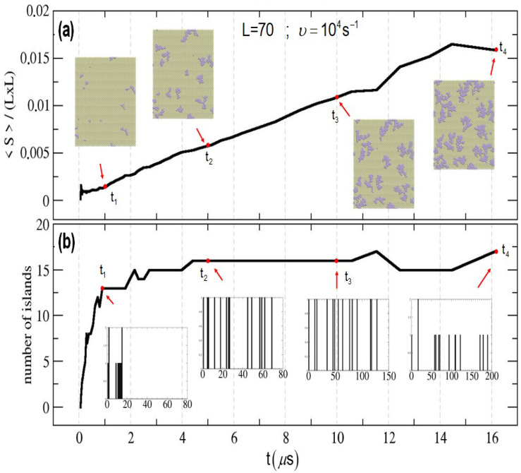 Figure 9
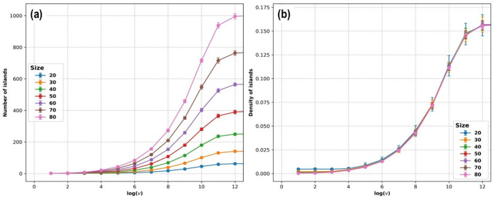 Figure 10
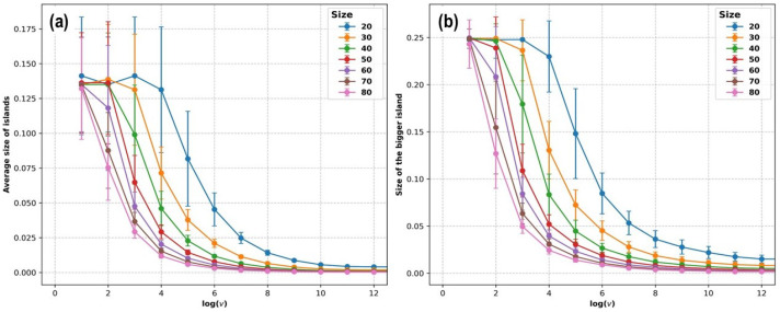 Figure 11
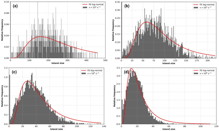 Figure 12
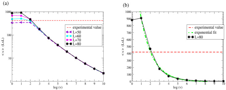 Figure 13
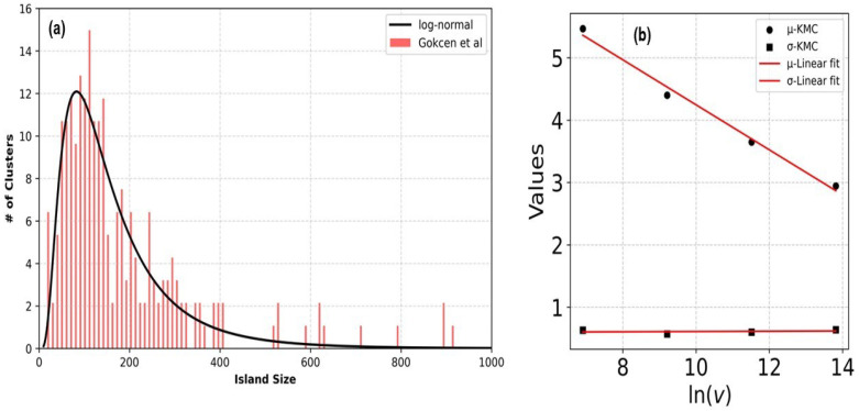 Figure 14
- —SECyT of the Universidad Nacional de Córdoba
Peer Reviews
No public reviews on file for this paper yet. If you reviewed it on a platform where reviews are public (OpenReview, ICLR, NeurIPS, ICML), you can paste yours below so the community can read it here.
Videos
No videos yet. Explain this paper in a talk, walkthrough, or lecture? Add one.
Taxonomy
TopicsCatalytic Processes in Materials Science · nanoparticles nucleation surface interactions · Advanced Chemical Physics Studies
1. Introduction
When the size of a metallic material decreases to the nanometric scale, it shows unique properties that cannot be observed in macroscopic-sized materials. The number of synthesis methods for these nanomaterials and their new and possible technological applications has increased over the last decade. For a long time, metallic ultra-thin overlayers, consisting of a two-dimensional structure of monoatomic height, have been considered the finest state of manipulation [1,2]. Nowadays, it is possible to obtain metallic ultra-thin structures (small 2D clusters) with diameters of a few nanometers in a quick and reproducible way [3,4]. The methodology used for this is the electrochemical deposition of foreign metals on another metal and/or semiconductor substrate. Several elementary steps, such as electron transfer, desolvation, and diffusion, are involved in this process, which in many cases implies the formation of a new phase through a nucleation and growth process. Understanding these phenomena would allow for a more efficient design of these compounds.
Platinum is one of the most commonly used metals because it catalyzes a large number of chemical and electrochemical reactions [5,6,7]. This metal is not an abundant element in nature, and consequently, it is expensive. So, much effort has been invested in making efficient catalytic surfaces to minimize the amount of used. Its deposition on less expensive, more abundant metals has been one of the strategies used to save . However, in general, the properties of ultra-thin overlayers differ from those of bulk ones due to diverse structural and quantum effects dominating their properties [1,2,3,4]. Fortunately, the electrocatalytic properties of a substrate are often greatly improved by the deposition of a monolayer of on its surface [3,4,8]. However, the size-dependent strain of nanoclusters has some effect on the energy of the d-band center and therefore on the activity of [9]. These facts show that it is necessary to deepen the understanding of the phenomena that control the morphology and size of the 2D clusters usually involved in nucleation and growth.
Since the interaction energy among atoms is stronger than the interaction between and other metal atoms, a three-dimensional growth or “Volmer–Weber” mechanism is expected under overpotential deposition (OPD) conditions [1,2,3,10,11]. Within this simplified picture of this electrochemical system, it appears, a priori, very difficult to produce ultra-thin films of on other less noble metals. However, a lot of experimental work has shown that this is possible, so the simplified view given above appears to be too simple to depict the actual electrochemical context [3]. Anions and cations dissolved in the electrolyte, pH, solubility, temperature, and other factors can play a key role in the growth of ultra-thin-film phases. Furthermore, the electrochemical environment offers great advantages due to the ability to easily create and manage very large electric fields at the interfaces. All these factors allow for the stabilization of certain structures and the modification of others in a way that is impossible under ultra-vacuum conditions.
The deposition of ultra-thin films of onto other less noble metals can be achieved through [12] electrochemical deposition (ED), spontaneous deposition (SD), and galvanic replacement (GR), also known as surface-limited redox replacement (SLRR). ED involves strict control of the deposition potential of the substrate on which the deposition occurs. Basically, a potential scan or step is applied to the substrate, which provides the electrons for the depositing ions, and a current transient occurs as a consequence of these events. The second method, SD, involves a first step, where the metal substrate is immersed in an electrolyte solution of a -containing electrolyte (i.e., ), and a second step, where an irreversible electrochemical reduction of to takes place. The structures that may be obtained with this procedure range from 2D clusters and ultra-thin films to multilayers [13,14,15,16,17]. The third method, GR, also called SLRR, involves the replacement of a previously adsorbed (via underpotential deposition (UPD)) sacrificial monolayer [3,4,8,18,19]. This method involves two stages: an electrochemical reduction leading to a UPD-deposited metal layer, which is later oxidized by the metal cations of the noble metal being deposited. The coverage of these thin films is controlled by the stoichiometry of the redox replacement reaction, the structure, and the coverage of the UPD monolayer. Thus, it is possible to obtain monolayers (or submonolayers) easily and quickly.
Regarding SD, Strbac et al. [16] showed that can be deposited on surfaces from . During the electrochemical reduction in the second step of SD, islands were formed homogeneously on via a nucleation and growth process, yielding nanosized islands with no preference for steps or other surface defects. However, Waibel et al. [10] showed through STM that deposition from or on or starts mainly at defects like step edges, and then three-dimensional clusters are formed. These are formed in different structures, such as [20], [10,20], [17], or [16] on , as well as on [10], in a broad range of cluster sizes and layer numbers. Similar behavior has been observed using other electrolytes, such as and [20].
Brankovic proposed that SD on is the result of two coupled half-cell reactions,
and
where the deposition mechanism can be proposed based on the fact that the reaction takes place on an oxide-free Ru surface [4,21]. However, in the case of SD on a surface, this cannot be assured. The potential for surface oxide formation on surfaces is more positive than the redox deposition potential, so oxide formation can interfere with the SD reaction.
SD has also been applied using the UPD of hydrogen preadsorbed onto a flat surface [22] of [23] and on Pd [22] nanoparticles, leading to the formation of an ultra-thin layer. More recently, Dai and Chen [24] showed that the SD approach can also be applied to achieve the growth of a atomic shell on nanoparticles using . In the latter work, the deposited atoms were uniformly distributed on the nanoparticles, with the coverage tunable by the electrolyte concentration and temperature. Similarly, Kim et al. [25] showed that when the -ion concentration is in the range – M, the deposits are nanoislands of monatomic height. In the concentration range – M, the deposits present mostly two-layer-thick nanofeatures. For higher concentrations, the deposits become wider and thicker. 2D clusters on -NPs with tunable coverage can also be designed on multiwall carbon nanotubes [26]. Therefore, SD can be used to generate various types of clusters and thin films on .
The ability to tune the size of 2D nanoclusters and/or the thickness of ultra-thin films requires a precise quantitative understanding of the phenomena that take place at the atomic level. An alternative to experimental work for accessing this information is the application of computational methods on the atomistic scale to simulate the surface reactions and transport phenomena of these electrochemical systems. Several numerical methods have been developed to simulate the formation of 2D nanoclusters or ultra-thin films. In general, two types of approaches have been used to simulate metal growth at the nanoscale: those that provide thermodynamic information, such as Monte Carlo (MC) or Grand Canonical Monte Carlo (GCMC) [27,28,29,30,31,32], and those that provide dynamic information, such as Molecular Dynamics (MD) or Kinetic Monte Carlo (KMC) [33,34,35,36,37,38,39,40]. MC and GCMC involve conducting numerical simulations using the introduction of random variables, whose values are assigned via the generation of random numbers. These methods provide information at the microscopic level for systems close to equilibrium, which may be converted into macroscopic information using concepts stemming from statistical mechanics (pressure, internal energy, etc.). MD is a deterministic approach that solves Newton’s equations (or some equivalent, depending on the assembly. To discretize time, time steps of the order of the femtosecond are required, which results in the dynamic behavior of the system being described on the nanosecond scale. However, many processes, especially those occurring in 2D nanocluster growth, take place on much larger time scales that are inaccessible through MD. For example, the experimental measurement of the activation energy for the diffusion of and atoms performed by Alonso et al. [41] resulted in values of eV and eV, respectively. Assuming a constant frequency factor on the order of s^−1^ at K, within absolute velocity theory, diffusional times can be estimated to be on the order of seconds for and on the order of hours for . Thus, MD does not appear to be an alternative to simulate the present phenomena.
On the other hand, the KMC technique [42] is stochastic in nature, and it is an efficient method for simulating physical phenomena that can be described in terms of Poisson processes. The theoretical foundation of the KMC technique was explained by Fichthorn in [43,44]. It is worth mentioning that with this technique, it is possible to reach experimental time scales, that is, on the order of seconds (or more). In Section 2, we will return to this topic. The KMC technique was employed by Timothy and Rikvold [37] to analyze metal deposition on a substrate seeded with 10-atom metal clusters. The authors analyzed the size distribution of 2D nanoclusters as a function of the energy barriers for surface diffusion, which ranged from eV to eV. Their results suggest that an energy barrier lower than eV would produce a uniform size distribution of the clusters. Effective lateral interactions were also employed by Zhang et al. [27] to successfully reproduce experimental transients originating from the adsorption of cations and sulfate anions. A more realistic approach to the metallic deposition of bidimensional layers, also using KMC simulations, was taken in subsequent work by Gimenez et al. [33,34]. In that work, embedded-atom method (EAM) potentials were employed to emulate the interaction between particles in a metallic - system. Also, Rafiee and Bashiri employed dynamic Monte Carlo simulations to study hydrogen production from formic acid decomposition on and [45,46]. They found the optimum temperature and pressure for hydrogen production and concluded that hydrogen is produced through direct dehydrogenation from formic acid.
Recent advances in KMC simulations led to the inclusion of atom-exchange phenomena. To account for collective surface diffusion processes, Treeratanaphitak et al. [39,40] included atom exchange and step-edge atom exchange in addition to nearest-neighbor hopping. This progress has led to a more realistic description of polycrystalline metal electrodeposition.
To the best of our knowledge, we have not detected work in the field of simulations devoted to understanding nucleation and growth on surfaces. This system is the final state of many experimental routines, such as ED, SD, and GR, which have found increasing technological applications over the last decade, as mentioned above. The simulation of a wide range of deposit morphologies that arise from various combinations of reaction rate, transport, and geometric parameters represents a gap in the theoretical literature. Thus, the combination of EAM potentials with KMC appears to be a promising tool for studying the present system in order to correlate theoretical results with experimental results. With this purpose, the subject of the present study is the analysis of the characteristics of the spontaneous deposition (SD) of small 2D nanoclusters of onto under different electrochemical conditions.
2. Model and Simulation Technique
2.1. General Model
The adsorption and diffusion of atoms on surfaces are modeled using kinetic Monte Carlo simulations. Surface alloys and multilayers are not allowed, since only one monolayer or submonolayer of atoms is considered. Two kinds of adsorption sites can be occupied by atoms: hollow hcp (hcp = “hexagonal close-packed”; refers to hollow sites with a gold atom in the layer below the upper one) or hollow fcc (fcc = “face-centered cubic”; refers to hollow sites without any atom in the layer below the upper one).
Adsorption is allowed on hcp sites that are unoccupied, as well as the three neighboring fcc sites, and on unoccupied fcc sites together with their hcp neighboring sites. Adsorption rates are considered constant for each simulation and independent of the environment. These values are parameterized.
Diffusion rates are allowed only between one hcp site and one of its three neighboring fcc sites, and vice versa. The diffusion velocities depend on the different environments (occupation of neighboring sites by other atoms).
2.2. Kinetic Monte Carlo Method
Monte Carlo methods are used as computational tools in many areas of physical chemistry. Although traditionally applied to obtain equilibrium properties, MC methods can also be used to study dynamic phenomena [43,44]. In the KMC method, every step consists of a random selection of one of many possible processes. The probability of a process being selected is directly proportional to its rate, which is represented as a fraction of a segment containing all processes that may occur in the system (see Figure 1). The rates of all possible processes are stored in an array of length , where is the total number of surface sites (where each component of the array is associated with a rate equal to if the site is available or 0 if it is not, i.e., when the site or one of its three neighboring sites is occupied), and is the total number of possible diffusion movements from each site to one of its three neighboring sites (where each component of the array is associated with a rate equal to —different for each environment—if there is a particle that can diffuse or 0 otherwise). Using a random number, the next process to occur is selected with a probability proportional to its rate.
Once the randomly chosen process has occurred, all possible processes are calculated and stored again in the corresponding fraction of the segment, and a time increment of is added, where u is a random number between 0 and 1, and is the sum of the rates of all possible processes. This choice of the time increment is due to the assumption that we are dealing with a Poisson process [42,43,44]. A general flowchart of the employed algorithm is shown in Figure 2.
To model the gold surface and the possible adsorption sites for atoms, a lattice containing three types of sites on the surface was generated. One type of site corresponds to the positions of the atoms of the substrate. The other two types of sites correspond to the possible positions at which adatoms can be adsorbed, that is, at and sites. The corresponding geometry is shown in Figure 3, where the positions of the atoms of the surface are also shown for clarity.
We say that a system is of size L when it is made of a plane that has fcc and hcp adsorption sites. The values of L analyzed here were 10, 20, 30, 40, 50, 60, 70, and 80. The adsorption of atoms is restricted in such a way that when a atom is adsorbed at an fcc (hcp) site, none of its three neighboring hcp (fcc) sites can be simultaneously occupied. This restriction is schematically depicted in Figure 3: the red arrows show the adsorption at the hcp site, its possible diffusion toward one of the three neighboring fcc sites, and the blocking of adjacent hcp sites; the black arrows show the adsorption at fcc sites.
For the diffusion of adatoms, the restriction of their motion is such that one atom adsorbed at an ( ) site can only diffuse toward one of its three ( ) neighboring sites (see Figure 3), with the condition that the final site and its corresponding neighbors (of the other type) must be empty to allow the move.
At each KMC step, two possible processes may occur: diffusion of an atom toward one of its neighboring sites if it is empty or adsorption of a atom. Thus, the adsorption process is considered irreversible. Surface alloying is not considered in the present approach, but it could be included in future formulations.
2.3. Energy Calculation
To calculate the velocities for adatom diffusion in different environments, a simple model based on embedded-atom method (EAM) calculations was used [47]. This method takes into account many-body effects; therefore, it represents the metallic bonding better than a pair potential. El-koraychy et al. [48] found that EAM and DFT results are in very good agreement, validating the embedded-atom approach for heteroepitaxial growth.
The EAM is a semi-empirical method that considers the total energy of an arrangement of N particles, calculated as the sum of energies corresponding to individual particles:
where is given by
where is called the embedding function and represents the energy necessary to embed atom i in the electronic density at the position at which this atom is located. The repulsion between ion cores is represented through a pair potential , which depends on the distance between the cores .
We employed the EAM within a lattice model, which is described in more detail in [31,32,33,34].
2.4. Diffusion Rate Calculations
The diffusion rates used in the simulation were calculated according to the different environments that an atom may encounter on the surface. Various configurations were taken into account according to the different possible arrangements of atoms near the starting and ending sites. Prior to the KMC simulation, for several configurations, the path followed by an atom to jump from one site to a neighboring one was traced, and the energy in each position was calculated, minimizing it with respect to z (the coordinate perpendicular to the surface plane). The activation energy, , was calculated as the difference between the saddle point and the initial minimum in the energy curve along the reaction coordinate. The vibrational frequency of the atom at the starting site was calculated by performing the harmonic approximation near the minimum of the curve without any neighbors. More details of this calculation procedure can be found in [33,34].
For each individual diffusion process, we considered that one atom positioned at a particular lattice site had three possibilities for moving toward one of the three nearest neighboring sites corresponding to the other sublattice (if the original position is on an fcc site, it can diffuse toward an hcp site, and vice versa). For each possible movement, eight neighboring sites were taken into account, four corresponding to the initial site and four corresponding to the final site. For each sublattice, every site has six nearest neighbors of the same sublattice, but the two closest to the other site must be unoccupied for the diffusion to be possible. Each neighboring site can have two possible occupation states: 0 (unoccupied) or 1 (occupied by a atom), totaling possible configurations, with each configuration corresponding to a particular value of the diffusion velocity.
Figure 4 shows a schematic representation of the diffusion process for a atom from one type of site to a neighboring site of the other type. The eight surrounding sites taken into account in the calculation of the velocity are shown and differentiated with the following labels: and for sites next to the initial site (which are of the same type as the initial site, either fcc or hcp) and for the four sites next to the final site (which are of the same type as the final site and opposite to the type of the initial site).
In order to calculate the diffusion velocities, the following considerations were made:
- The activation energy in the absence of any neighbors was assumed to be eV. This corresponds to the value obtained from the EAM calculation for the motion of a single atom between two neighboring adsorption sites on a surface in the absence of any neighbors.
- The vibrational frequency of the atom at the starting site in the absence of any neighbors was s^−1^, obtained from the same EAM calculations. The assumption here was that changes in due to the presence of neighboring atoms are negligible compared with changes in the activation energy. So, we considered the same vibrational frequency for all possible configurations.
- The fastest diffusion process was assumed to be the diffusion from a site without neighbors to a site surrounded by 4 atoms. The activation energy for this process was set to zero.
- Two types of contributions to the activation energy were assumed to arise when the neighboring sites of the initial site are occupied, say and . These were obtained from EAM calculations, yielding eV/atom and eV/atom.
Thus, the activation energy is calculated as
where is the number of atoms adsorbed on the two type-1 neighboring sites of the initial site (those sites located farther away from the arriving site), is the number of atoms adsorbed on the two type-2 neighboring sites of the initial site (those sites located closer to the arriving site), and is the number of atoms adsorbed on the four neighboring sites of the final site.
Taking into account the parameters indicated in Table 1 and the activation energy calculated according to Equation (5), the velocity for each possible diffusion event was calculated as . Here, the considered temperature was K, so eV.
The parameters listed in Table 1 were selected according to the method described in the first paragraph of this section for some particular configurations. In particular, the values of and correspond to the case of diffusion of one single atom on the surface in the absence of nearest neighbors. For the value of the parameter , the activation energy corresponding to the configuration with two nearest neighbors at type-1 initial sites was taken into account (the value of the parameter was calculated as ). For , the procedure was the same, but for type-2 sites. On the other hand, the parameter was calculated as in order to obtain the maximum possible value of velocity (that with eV) in the case of four nearest neighbors next to the arriving site and none next to the starting site.
2.5. Deposition Rates
Let us consider ions in the electrolytic solution, generally complexed as , with a constant activity ( = ) at a temperature T. The electrochemical deposition/dissolution rates at a given electrode potential (E), measured against a reference electrode, are given by the following equations:
where the values of are the activation energies for the ion transfer from the solution to the crystal, or vice versa, at ; is the charge transfer coefficient; is the activity of metal ions in the electrolyte; and and are the rate constants for the deposition and the dissolution reaction at each site [1,34].
The above equations indicate that each site is subject to an equilibrium between deposition and dissolution. This equilibrium can be altered by the electrode potential. It should be noted that the simulations were performed at potentials where . According to Equations (6) and (7), this occurs because the exponential term in the electric potential in the reaction is the dominant one. Under these conditions, one can consider .
In the present work, we considered different values of ( s^−1^, with ). These values correspond to different possible electrode potentials, E. The dissolution rate was neglected. Thus, in the present model, each site was subject to two types of movements: diffusional, where the (surface) diffusion rates were calculated depending on the environment, and deposition (or adsorption), whose rate was introduced parametrically.
3. Results
3.1. Diffusion Rates
Figure 5 shows the rate values for the diffusion of a atom on the surface, with six possible environments. It can be seen that the diffusion rate on a clean surface is on the order of s^−1^, whereas a nearest-neighboring atom located close to the initial state of the movement decreases the probability of diffusion to a rate on the order of s^−1^ or s^−1^, depending on the location of the neighbor. On the other hand, a atom located near the site of arrival increases the diffusion rate to a rate of s^−1^. From configurations (b), (d), and (e) in Figure 5, we learn that the detachment of a atom from a cluster is almost impossible.
3.2. Pt Deposition on Au(111)
The formation of 2D clusters on surfaces was analyzed at different deposition rates on systems of different sizes , corresponding to substrates with supercells containing between 100 ( ) and 6400 ( ) atoms. Although the system was, in principle, infinite, since the simulation supercell was repeated with periodic boundary conditions in two dimensions (x and y), finite-size effects appeared, since the largest adsorbate island cannot be larger than the dimension of the supercell employed. We analyze this problem in the following paragraphs. Since the diffusion rates were fixed due to the fact that they were all calculated based on selected parameters, the free variable taken into account was the deposition rate , which is the rate assigned to the adsorption of a single atom from the solution and was taken as a parameter to explore the behavior of the system. The values considered were s^−1^, with . Although larger values are physically unrealistic because they correspond to very large experimental overpotentials, they were included anyway to provide a view of the velocity ranges where different behaviors may be expected.
3.2.1. Time Evolution
Figure 6 shows snapshots of the simulation for platinum adsorption for a system size and a deposition rate s^−1^, corresponding to different stages of the KMC simulation at different times, as indicated. It can be observed that a few islands with dendritic-type structures formed for a final deposition time on the order of milliseconds. The shape of the islands can be explained by the fact that free atoms on the surface can diffuse until they reach an existing island, and then diffusion around the steps or leaving the island becomes very difficult due to the low velocities associated with these processes.
On the other hand, Figure 7 shows snapshots of the final states of the simulations for platinum adsorption for a system size and deposition rates s^−1^, s^−1^, s^−1^, and s^−1^. For the lowest deposition rate, only one island can be observed, while for higher deposition rates, several small islands can be seen.
Here, the average island size is defined as
where is the total number of islands (including monomers) and is the size (number of atoms) of the j-th island.
Figure 8 and Figure 9 show the time evolution of the average island size (normalized by the system size) and the total number of islands for two cases used as examples: a system size and a deposition rate s^−1^ (Figure 8), and a system size and a deposition rate (Figure 9). Snapshots of the state of the surface and histograms for the island distribution are also included for selected times.
For the simulation shown in Figure 8, only one island is present until s. At that particular time, a second island is formed. So, the average island size increases nearly linearly until s, then decreases abruptly due to the formation of a second island, and subsequently continues to increase linearly but with a lower slope compared to the initial stage.
For the simulation shown in Figure 9, as the system size is larger and the deposition rate is higher, a larger number of smaller islands than in the previous example is observed. The total number of islands initially increases, corresponding to a nucleation and growth stage, and for times around s, this number remains more or less constant, corresponding to a growth stage (the existing islands continue growing in size, but no new islands are formed).
3.2.2. Average Values in Final States
Figure 10 and Figure 11 show the total number of islands, the density of islands, the average size of islands, and the size of the biggest island in the final state (which corresponds to ; the simulation ends when the last particle necessary to reach this coverage degree adsorbs) as a function of the logarithm of the deposition rate , for system sizes corresponding to and 80, with each case averaged over 100 KMC simulations.
In Figure 10a, it can be seen that the total number of islands increases with the deposition rate. The system size also influences the number of islands. But, as can be seen in Figure 10b, when the island density is considered (the number of islands normalized by the system size), the different curves overlap, except for the case when (and to a lesser extent for ), where the density is higher than that observed for the other system sizes. This shows that finite-size effects are only evident for the smallest system sizes but are negligible for most of the system sizes considered here.
Figure 11 shows the results obtained from the simulations for the average island size and the maximum island size , normalized by the size of the simulation box, . Both plots show qualitatively similar behavior, with a plateau at lower values of , followed by a decrease, and finally asymptotic behavior toward a small value for very high rates. The plateau at lower values of is a result of the finite-size effect: if the deposition rate is low enough, a single island covers the whole simulation supercell, and the physical relevance of the simulation is lost. The value for low values of indicates a single large island with a size almost given by the coverage degree, while a smaller value of for lower values of (Figure 11a) indicates the presence of a few small islands or even single atoms, which are not shown in Figure 11b.
Figure 12 shows histograms for the island size distribution at the final state for four different deposition rates. In these cases, the system size is , and 100 KMC simulations are averaged. As can be seen, for low deposition rates, the size distribution of islands becomes wide, and the island sizes reach relatively large values. As the deposition rate increases, the size distribution becomes narrower, and the mean shifts toward lower values.
Figure 13 shows a plot of the average island sizes (the same cases as in Figure 11a, but multiplied by ), together with the value corresponding to the experimental case. In Figure 13a, the four largest system sizes are shown together on a logarithmic scale on the y-axis, and it can be seen that, except for the lower values of , the system size effects are negligible.
Concerning the comparison with the experiments, the theoretical histograms in Figure 12 show remarkable features, which were compared with those of similar experimental results from Ref. [18]. These results are reproduced in Figure 14. In this figure, we see that the shape of the distribution of the clusters obtained in [18], depicted in red bars, strongly resembles the distribution curves in Figure 12.
To seek a more quantitative comparison, we employ a lognormal distribution function used in the literature to describe the distribution of nanocrystal clusters [49,50]:
where S represents the island size, is the mean value of the logarithm of the island sizes, and is the standard deviation. The red curves in Figure 12 correspond to the fitting of the numerical data to Equation (9), and the parameters and are given in Table 2.
These parameters are represented as a function of the logarithm of the deposition rate in the inset of Figure 14. It can be seen that while is insensitive to , shows a linear dependence on . When the same fitting is applied to the experimental data from Figure 14, we obtain and . Thus, we find remarkable agreement between the of the experimental distribution and the theoretical values reported in Table 2, indicating that the simulations captured the physical features of the experiment.
4. Conclusions
Kinetic Monte Carlo simulations for the deposition and diffusion of atoms on surfaces were performed to study the electrochemical deposition and spontaneous island formation of platinum on gold. On one hand, the diffusion rates were calculated using absolute rate theory, with some parameters based on EAM calculations. On the other hand, the deposition rates were treated as a parameter that could take several possible values (emulating different experimental conditions).
The time evolution and final states for the coverage degree were studied for different values of . In all cases, the morphology of the deposited island was found to be rather ramified, instead of forming compact islands. The density of islands at the final state (for ) increased with increasing , and the curves were found to be independent of the system size, except for (very small). The average island size (normalized by system size) as a function of was approximately constant for low deposition velocities and then decreased as increased, depending on the system size. The island size distribution at the final state was broader and tended toward higher values at lower .
The reference list from the paper itself. Each links out to its DOI / PubMed record.
- 1Budevski E. Staikov G. Lorenz W.J. Electrochemical Phase Formation and Growth VCH Weinheim, German 1996
- 2Staikov G. Lorenz W.J. Budevski E. Imaging of Surfaces and Interfaces—Frontiers of Electrochemistry Ross P. Lipkowski J. Wiley-VCH New York, NY, USA 1999 Volume 5
- 3Oviedo O.A. Reinaudi L. Garcia S. Leiva E.P.M. Underpotential Deposition, From Fundamentals and Theory to Applications at the Nanoscale Serie Monographs in Electrochemistry Springer Berlin/Heidelberg, Germany 2016
- 4Brankovic S. Electrocatalysis: Novel Synthetic Methods in Electrocatalysis: Novel Synthetic Methods Springer Berlin/Heidelberg, Germany 2014
- 5Kowal A. Li M. Shao M. Sasaki K. Vukmirovic M.B. Zhang J. Marinkovic N.S. Liu P. Frenkel A.I. Adzic R.R. Ternary Pt/Rh/Sn O 2 electrocatalysts for oxidizing ethanol to CO 2Nat. Mater.2009832533010.1038/nmat 235919169248 · doi ↗ · pubmed ↗
- 6Adzic R. Zhang J. Sasaki K. Vukmirovic M.B. Shao M. Wang J.X. Nilekar A.U. Mavrikakis M. Valerio J.A. Uribe F. Platinum monolayer fuel cell electrocatalysts Top. Catal.20074624910.1007/s 11244-007-9003-x · doi ↗
- 7Sasaki K. Wang J.X. Naohara H. Marinkovic N. More K. Inada H. Adzic R.R. Recent advances in platinum monolayer electrocatalysts for oxygen reduction reaction: Scale-up synthesis, structure and activity of Pt shells on Pd cores Electrochim. Acta 201055264510.1016/j.electacta.2009.11.106 · doi ↗
- 8Gokcen D. Yuan Q. Brankovic S.R. Nucleation of Pt monolayers deposited via surface limited redox replacement reaction J. Electrochem. Soc.2014161 D 3051 D 305610.1149/2.007407 jes · doi ↗