Forensic comparison analysis of smokeless powders by gel permeation chromatography and likelihood ratio evaluation methods
Hongling Guo, Ping Wang, Can Hu, Hongcheng Mei, Yajun Li, Jun Zhu

TL;DR
This study explores using gel permeation chromatography and likelihood ratios to compare smokeless powders for forensic analysis in China.
Contribution
The paper introduces a novel forensic method for comparing smokeless powders based on polymer properties rather than trace compounds.
Findings
Gel permeation chromatography measured molecular weights and PDI values of 79 smokeless powder samples.
Likelihood ratio evaluation helped interpret data for forensic comparisons between powders.
The method shows potential for linking powders without relying on trace compound analysis.
Abstract
In China, the use of smokeless powders for making homemade ammunition and bombs is an incipient criminal practice. One of the key tasks of analyzing smokeless powders in forensic sciences is to make comparisons between them, providing information about their source or establishing a link between two different smokeless powders seized at different locations. The main component of smokeless powders is nitrocellulose (NC) no matter what type of the smokeless powder is. As a kind of polymer, NC may have different molecular weights and polydispersity index (PDI) values, which could help the identification and differentiation of the smokeless powders. In this study, weight-average molecular weights (Mw), number-average molecular weights (Mn), and PDI value of 79 propellants samples from different sources were measured by gel permeation chromatography, and likelihood ratio evaluation method…
Genes, proteins, chemicals, diseases, species, mutations and cell lines named across the full text — each resolved to its canonical identifier and authoritative record.
Click any figure to enlarge with its caption.
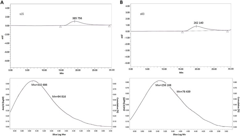 Figure 1
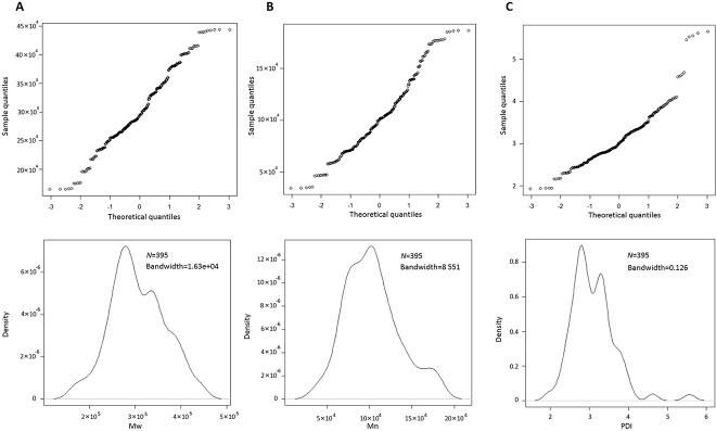 Figure 2
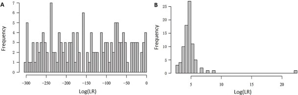 Figure 3
| Sample | Manufacturer | Cartridge | Production year | Caliber | Sample | Manufacturer | Cartridge category | Production | Caliber (mm) |
|---|---|---|---|---|---|---|---|---|---|
| s1 | 121 | 51 pistol | 1958 | 7.62 | s41 | 81 | 59 rifle | 1966 | 9.00 |
| s2 | 121 | 51 pistol | 1963 | 7.62 | s42 | 911 | 56 rifle | 1968 | 5.60 |
| s3 | 121 | 51 pistol | 1964 | 7.62 | s43 | 911 | 56 rifle | 1979 | 5.60 |
| s4 | 121 | 51 pistol | 1965 | 7.62 | s44 | C | Sporting rifle | Unknown | 5.60 |
| s5 | 121 | 51 pistol | 1970 | 7.62 | s45 | CJ | SS109 rifle | 2000 | 5.60 |
| s6 | 121 | 51 pistol | 1972 | 7.62 | s46 | Czech Republic | Pistol | Unknown | 7.65 |
| s7 | 121 | 51 pistol | 1979 | 7.62 | s47 | KKJ | Nail | Unknown | 6.80 × 18 |
| s8 | 121 | 51 pistol | 1981 | 7.62 | s48 | KKJ | Nail | Unknown | 6.30 × 16 |
| s9 | 121 | 51 pistol | 1987 | 7.62 | s49 | KKJ | Nail | Unknown | 6.3 0× 16 |
| s10 | 121 | 51 pistol | 1991 | 7.62 | s50 | LY | Parabellum pistol | 1994 | 9.00 |
| s11 | 121 | 51 pistol | 2018 | 7.62 | s51 | NS | Nail | Unknown | 6.80 × 11 |
| s12 | 121 | Revolver pistol | 2005 | 9.00 | s52 | NS | Nail | Unknown | 6.80 × 11 |
| s13 | 121 | DAP92 pistol | 2019 | 9.00 | s53 | NS | Nail | Unknown | 6.80 × 18 |
| s14 | 121 | DAP92 pistol | 2018 | 9.00 | s54 | NS | Nail | Unknown | 6.80 × 18 |
| s15 | 121 | 64 pistol | 2007 | 7.62 | s55 | NS | Nail | Unknown | 5.60 × 16 |
| s16 | 121 | 64 pistol | 1990 | 7.62 | s56 | NS | Nail | Unknown | 5.60 × 16 |
| s17 | 121 | 64 pistol | 1990 | 7.62 | s57 | NS | Nail | Unknown | 6.30 × 16 |
| s18 | 121 | 64 pistol | 1992 | 7.62 | s58 | NS | Nail | Unknown | 5.60 × 16 |
| s19 | 121 | 64 pistol | 1995 | 7.62 | s59 | NS | Nail | Unknown | 6.80 × 11 |
| s20 | 121 | 64 pistol | 1996 | 7.62 | s60 | NS | Nail | Unknown | 5.60 × 16 |
| s21 | 121 | 64 pistol | 1990 | 7.62 | s61 | NS | Nail | Unknown | 6.80 × 11 |
| s22 | 121 | 92 rifle | 2002 | 7.62 | s62 | NS | Nail | Unknown | 6.80 × 11 |
| s23 | 301 | 64 pistol | 1980 | 7.62 | s63 | NS | Nail | Unknown | 6.80 × 11 |
| s24 | 301 | 64 pistol | 1987 | 7.62 | s64 | Ω | Sporting rifle | Unknown | 5.60 |
| s25 | 311 | 64 pistol | 1989 | 7.62 | s65 | Double Ring | Sporting rifle | Unknown | 5.60 |
| s26 | 311 | 64 pistol | 1992 | 7.62 | s66 | △ | Sporting rifle | Unknown | 5.60 |
| s27 | 311 | 64 pistol | 1994 | 7.62 | s67 | △ | Sporting rifle | Unknown | 5.60 |
| s28 | 311 | 64 pistol | 2004 | 7.62 | s68 | YRD | Nail | Unknown | 6.80 × 11 |
| s29 | 611 | 56 rifle | 1967 | 7.62 | s69 | YRD | Nail | Unknown | 6.80 × 11 |
| s30 | 671 | 53 pistol | 2013 | 7.62 | s70 | YRD | Nail | Unknown | 6.8 0× 11 |
| s31 | 71 | 56 rifle | 1956 | 7.62 | s71 | YRD | Nail | Unknown | 6.80 × 18 |
| s32 | 724 | DAP92 pistol | 2007 | 5.80 | s72 | YRD | Nail | Unknown | 6.80 × 18 |
| s33 | 791 | 9 mm pistol | 2016 | 9.00 | s73 | YRD | Nail | Unknown | 5.60 × 16 |
| s34 | 791 | 56 pistol | 1988 | 7.62 | s74 | YRD | Nail | Unknown | 5.60 × 16 |
| s35 | 791 | SS109 rifle | 2001 | 5.56 | s75 | YRD | Nail | Unknown | 5.60 × 16 |
| s36 | 791 | DCV05 pistol | 2008 | 5.80 | s76 | YRD | Nail | Unknown | 6.30 × 16 |
| s37 | 791 | 95 pistol | 2016 | 5.80 | s77 | YRD | Nail | Unknown | 6.30 × 16 |
| s38 | 791 | Pistol | 2014 | 5.80 | s78 | YRD | Nail | Unknown | 5.60 × 16 |
| s39 | 791 | DVP88A pistol | 2017 | 5.80 | s79 | YRD | Nail | Unknown | 5.60 × 16 |
| s40 | 81 | 56 rifle | 1964 | 7.62 | |||||
| Series number | Mw | Mn | PDI | Series number | Mw | Mn | PDI | ||||||
|---|---|---|---|---|---|---|---|---|---|---|---|---|---|
| Mean | RSD (%) | Mean | RSD (%) | Mean | RSD (%) | Mean | RSD (%) | Mean | RSD (%) | Mean | RSD (%) | ||
| s1 | 377 609 | 0.048 | 113 399 | 0.287 | 3.33 | 0.300 | s41 | 342 815 | 0.058 | 126 978 | 0.131 | 2.70 | 0 |
| s2 | 384 420 | 0.040 | 120 826 | 0.222 | 3.18 | 0.314 | s42 | 351 666 | 0.046 | 133 901 | 0.191 | 2.63 | 0.380 |
| s3 | 401 652 | 0.076 | 161 637 | 0.152 | 2.48 | 0.403 | s43 | 313 484 | 0.057 | 93 209 | 0.245 | 3.36 | 0.298 |
| s4 | 403 037 | 0.053 | 185 683 | 0.098 | 2.17 | 0 | s44 | 340 849 | 0.086 | 139 437 | 0.083 | 2.44 | 0 |
| s5 | 411 389 | 0.049 | 177 828 | 0.136 | 2.31 | 0 | s45 | 342 363 | 0.036 | 117 984 | 0.265 | 2.90 | 0.345 |
| s6 | 359 511 | 0.061 | 92 272 | 0.415 | 3.90 | 0.513 | s46 | 281 623 | 0.069 | 106 987 | 0.206 | 2.63 | 0.380 |
| s7 | 355 935 | 0.055 | 126 792 | 0.120 | 2.81 | 0.356 | s47 | 330 161 | 0.061 | 116 413 | 0.230 | 2.84 | 0.352 |
| s8 | 351 566 | 0.073 | 119 337 | 0.144 | 2.95 | 0.339 | s48 | 301 918 | 0.076 | 110 671 | 0.223 | 2.73 | 0 |
| s9 | 348 915 | 0.050 | 109 151 | 0.216 | 3.20 | 0.313 | s49 | 258 148 | 0.072 | 106 540 | 0.191 | 2.42 | 0 |
| s10 | 380 216 | 0.048 | 143 308 | 0.154 | 2.65 | 0.377 | s50 | 307 260 | 0.099 | 110 372 | 0.207 | 2.78 | 0.360 |
| s11 | 373 633 | 0.087 | 102 717 | 0.156 | 3.64 | 0.275 | s51 | 294 956 | 0.103 | 96 073 | 0.227 | 3.07 | 0.326 |
| s12 | 200 888 | 0.105 | 82 939 | 0.276 | 2.42 | 0.413 | s52 | 322 763 | 0.085 | 165 853 | 0.150 | 1.95 | 0.513 |
| s13 | 176 096 | 0.071 | 58 190 | 0.605 | 3.03 | 0.660 | s53 | 284 187 | 0.068 | 88 221 | 0.319 | 3.22 | 0.311 |
| s14 | 334 696 | 0.065 | 124 723 | 0.113 | 2.68 | 0.373 | s54 | 283 987 | 0.091 | 82 817 | 0.333 | 3.43 | 0.292 |
| s15 | 332 843 | 0.090 | 94 837 | 0.143 | 3.51 | 0.285 | s55 | 326 248 | 0.065 | 117 499 | 0.139 | 2.78 | 0 |
| s16 | 341 562 | 0.058 | 107 293 | 0.191 | 3.18 | 0.314 | s56 | 290 207 | 0.071 | 87 382 | 0.208 | 3.32 | 0.301 |
| s17 | 329 471 | 0.025 | 100 018 | 0.274 | 3.30 | 0.303 | s57 | 256 346 | 0.087 | 76 481 | 0.235 | 3.35 | 0.299 |
| s18 | 334 435 | 0.076 | 144 988 | 0.139 | 2.31 | 0.433 | s58 | 282 871 | 0.053 | 101 802 | 0.200 | 2.78 | 0.360 |
| s19 | 244 943 | 0.146 | 60 213 | 0.367 | 4.07 | 0.491 | s59 | 260 301 | 0.095 | 79 791 | 0.150 | 3.26 | 0 |
| s20 | 271 747 | 0.107 | 70 753 | 0.293 | 3.84 | 0.260 | s60 | 294 477 | 0.041 | 103 959 | 0.181 | 2.83 | 0 |
| s21 | 233 226 | 0.069 | 67 753 | 0.304 | 3.44 | 0.291 | s61 | 235 659 | 0.076 | 71 735 | 0.236 | 3.29 | 0.304 |
| s22 | 222 341 | 0.063 | 59 027 | 0.522 | 3.77 | 0.531 | s62 | 262 356 | 0.048 | 85 378 | 0.166 | 3.07 | 0 |
| s23 | 275 370 | 0.076 | 74 728 | 0.450 | 3.69 | 0.542 | s63 | 248 470 | 0.043 | 79 579 | 0.388 | 3.12 | 0.321 |
| s24 | 264 591 | 0.073 | 91 035 | 0.334 | 2.91 | 0.344 | s64 | 279 183 | 0.111 | 93 356 | 0.310 | 2.99 | 0.334 |
| s25 | 269 582 | 0.145 | 105 071 | 0.071 | 2.57 | 0 | s65 | 255 071 | 0.097 | 65 005 | 0.328 | 3.92 | 0.255 |
| s26 | 259 055 | 0.095 | 74 186 | 0.301 | 3.49 | 0.287 | s66 | 237 862 | 0.110 | 71 234 | 0.458 | 3.34 | 0.599 |
| s27 | 285 431 | 0.089 | 101 283 | 0.230 | 2.82 | 0.355 | s67 | 264 637 | 0.079 | 71 254 | 0.431 | 3.71 | 0.539 |
| s28 | 196 135 | 0.103 | 35 208 | 0.750 | 5.57 | 0.718 | s68 | 275 158 | 0.100 | 83 773 | 0.267 | 3.28 | 0.305 |
| s29 | 217 829 | 0.045 | 46 652 | 0.474 | 4.67 | 0.428 | s69 | 301 821 | 0.068 | 100 090 | 0.244 | 3.01 | 0.332 |
| s30 | 265 380 | 0.067 | 81 914 | 0.239 | 3.24 | 0.309 | s70 | 292 491 | 0.071 | 104 005 | 0.312 | 2.81 | 0.356 |
| s31 | 379 797 | 0.103 | 128 363 | 0.172 | 2.96 | 0.338 | s71 | 255 273 | 0.091 | 69 449 | 0.304 | 3.67 | 0.272 |
| s32 | 443 478 | 0.041 | 173 152 | 0.148 | 2.56 | 0.391 | s72 | 286 906 | 0.105 | 75 951 | 0.371 | 3.78 | 0.265 |
| s33 | 399 947 | 0.046 | 157 063 | 0.148 | 2.55 | 0.392 | s73 | 287 967 | 0.090 | 88 019 | 0.309 | 3.27 | 0.306 |
| s34 | 386 746 | 0.079 | 139 256 | 0.161 | 2.78 | 0 | s74 | 282 806 | 0.092 | 83 101 | 0.183 | 3.40 | 0.294 |
| s35 | 381 586 | 0.075 | 138 978 | 0.176 | 2.74 | 0.365 | s75 | 278 265 | 0.100 | 95 752 | 0.255 | 2.91 | 0.344 |
| s36 | 439 878 | 0.062 | 176 778 | 0.181 | 2.49 | 0 | s76 | 304 709 | 0.087 | 107 305 | 0.213 | 2.84 | 0.352 |
| s37 | 415 211 | 0.054 | 152 148 | 0.172 | 2.73 | 0 | s77 | 305 580 | 0.105 | 105 267 | 0.190 | 2.90 | 0 |
| s38 | 331 491 | 0.091 | 123 379 | 0.125 | 2.69 | 0.372 | s78 | 236 087 | 0.125 | 70 598 | 0.384 | 3.34 | 0.299 |
| s39 | 346 181 | 0.052 | 122 728 | 0.277 | 2.82 | 0.355 | s79 | 309 538 | 0.058 | 101 229 | 0.169 | 3.06 | 0.327 |
| s40 | 165 500 | 0.147 | 47 126 | 0.382 | 3.51 | 0.570 | |||||||
- —Grant Technology Research Project of the Ministry of Public Security, China
- —Grant Double Ten Project of Ministry of Public Security, China
- —Grant Central Public-Interest Scientific Institution Basal Research Fund
- —Ministry of Public Security under Grant Basic Work Plan for Strengthening Police Force of Ministry of Public Security, China
Peer Reviews
No public reviews on file for this paper yet. If you reviewed it on a platform where reviews are public (OpenReview, ICLR, NeurIPS, ICML), you can paste yours below so the community can read it here.
Videos
No videos yet. Explain this paper in a talk, walkthrough, or lecture? Add one.
Taxonomy
TopicsBiochemical effects in animals · Analytical Chemistry and Chromatography · Toxic Organic Pollutants Impact
Introduction
Smokeless powders (SLPs) are often used in civilian and military ammunition. In China, they are the most common low explosives used to fabricate improvised explosive devices such as pipe bombs and home-made ammunition due to their relative ease of accessibility. As a consequence, SLPs are commonly encountered in the investigation of many firearm- and explosive-related crimes, making their examination, analysis and profiling very important from a forensic perspective. It is common to make comparisons between the SLPs used in the devices and those available in suspect’s houses or manufacturing places for forensic investigations. These procedures may help investigators establish a link between two different SLPs seized at different locations.
The major classes of compounds in smokeless powders include energetics, stabilizers, plasticizers, flash suppressants, deterrents, opacifiers, and dyes [1]. According to the main chemical substances in the energetic class of compounds, smokeless powders can be classified into three different types: single-base, double-base, and triple-base. A single-base powder contains nitrocellulose (NC), a double-base powder contains nitrocellulose and nitroglycerin, and a triple-base powder contains nitrocellulose, nitroglycerine, and nitroguanidine. NC is the main component no matter what type of the smokeless powder is. It was reported that infrared spectroscopy, chromatography, and mass spectroscopy have been commonly used for the determination of different ingredients in smokeless powders [2–5]. These above-mentioned methods mainly focus on identifying the additives in SLPs and disregard the main component of NC. Due to the low amount and limited variation of additives across manufacturers and batches [6], the chemical characterization of NC itself might significantly increase the options for forensic comparison and attribution.
NC is a structurally complex polymer that is produced by the nitration of plant-based cellulose using concentrated nitric and sulfuric acid [7]. Different from small molecular compounds, which have exact molecular weight values, polymer molecular weight is defined as a distribution rather than a specific number because polymerization occurs in such a way to produce different chain lengths [8], which is an important feature of polymer compounds. The concept of molecular weight of polymer materials is usually characterized by weight-average molecular weight (Mw) or number-average molecular weight (Mn) and its distribution property, the polydispersity index (PDI). Gel permeation chromatography (GPC) is a useful and robust technique for polymer material analysis and has been investigated for many years [7, 9–11]. However, very few papers have reported the analysis of NC by GPC [7, 12]. In this study, we explore the possibility and suitability using Mw, Mn and PDI data of NC and likelihood ratio (LR) calculation method to make further discrimination and data evaluation between SLPs.
Materials and methods
Collection and preparation of samples
We use propellant samples with known sources to test the validity of the methods used. Detailed information, ⁓79 collected smokeless powders were presented in Table 1. The powders were taken out from the cartridges by using a cartridge puller. The SLP samples were dissolved in tetrahydrofuran (THF) at room temperature with a concentration ⁓1 mg/mL and left overnight to dissolve.
GPC measurement
All SLPs were analyzed on the Waters 1515 GPC instrument (Waters Corp., Milford, MA, USA), consisting of a 2414 Refractive Index (RI) detector (Waters Corp.). In the experiment, the series connection of column of Waters Styragel HT3 (7.8 × 300 mm), Styragel HT4 (7.8 × 300 mm) and Styragel HT5 (7.8 × 300 mm) were used. The column and detedctor temperatures were both 35°C. The mobile phase was THF. The flow rate was ⁓1 mL/min. The collection time was 30 min and the sample volume for GPC measurement was 100 μL. Polystyrene standards (PS770-PS1350000) for GPC calibration were used. Each sample was measured with five replicates.
Inter- and intra-day precision evaluation was carried out using three different samples with sample number s1, s38, and s63. For intra-day precision, these three samples were measured five times in 1 day and the relative standard deviation (RSD,%) was calculated. The three samples were analyzed on five consecutive days and the data were used to evaluate the inter-day precision.
LR calculation
LR calculation was applied in this work to give a quantitative evaluation of the analysis data. For comparison work, it was used to evaluate the strength of evidential data based on two contrasting hypotheses: (i) prosecution proposition (H_1_) proposed that the compared SLP samples came from the same source; (ii) defense proposition (H_2_) proposed that they had different sources. The general LR formula can be expressed by Eq 1:
\documentclass[12pt]{minimal} \usepackage{amsmath} \usepackage{wasysym} \usepackage{amsfonts} \usepackage{amssymb} \usepackage{amsbsy} \usepackage{upgreek} \usepackage{mathrsfs} \setlength{\oddsidemargin}{-69pt} \begin{document} \begin{equation*} LR=\frac{f\left(E\ \right|{H}_1)}{f\left(E\ |\ {H}_2\right)} \end{equation*}\end{document}where, E is the evidence obtained from the Mw, Mn and PDI values. The definition indicates that values of LR > 1 support H_1_, while values of LR < 1 support H_2_. A value of LR = 1 does not provide support for either proposition. The magnitude (higher or lower) of the value of LR indicates increased support for the evidence (H_1_ or H_2_). The exact LR calculation model can refer to the paper published in 2023 by our group [13]. The LR model in this work was built based on the multivariate data of Mw, Mn and PDI of 79 SLP samples. LR calculation involving these three variables were calculated by programming with R software (https://www.r-project.org/).
The within-object distribution was assumed to be normal. The between-object distribution of the data was estimated by Quantile-Quantile (Q-Q) plot to check if they conformed to a normal distribution. Kernel density estimation (KDE) using Gaussian kernels was employed if between-object distribution could not be estimated by a normal distribution (for details see [14]).
Results and discussion
Mw, Mn, and PDI analysis of different SLP samples
The inter-day precision for Mw, Mn, and PDI of sample s1, s38, and s63 was 0.052%, 0.295% and 0.368%, respectively; and the intra-day precision was 0.095%, 0.457%, and 0.579%, respectively, which demonstrated that GPC method had good reproducibility. Seventy-nine SLP samples were analyzed by GPC and the mean values of Mw, Mn and PDI were listed in Table 2. The GPC instrumentation can provide Mw and Mn at the same time, and PDI can be easily calculated. The PDI is used as a measure of the broadness of a molecular weight distribution of a polymer and is defined by \documentclass[12pt]{minimal} \usepackage{amsmath} \usepackage{wasysym} \usepackage{amsfonts} \usepackage{amssymb} \usepackage{amsbsy} \usepackage{upgreek} \usepackage{mathrsfs} \setlength{\oddsidemargin}{-69pt} \begin{document} PDI=\frac{M_w}{M_n}\end{document} . The larger the PDI is, the broader the molecular weight disperses. In this study, significant scattering of Mw, Mn and PDI was observed: Mw ranged from 165 500 to 443 478, Mn ranged from 35 208 to 185 683, and PDI from 1.95 to 5.57. Figure 1 showed the chromatograms of samples s15 and s63, having different Mw, but close PDI (with a value ⁓3.3).
Chromatograms of samples s15 (A) and s63 (B). Mw: molecular weights; Mn: number-average molecular weights.
LR calculation
Q-Q plots and KDE methods were used to evaluate if the data conformed to a normal distribution. The Q-Q plots and KDE curves for Mw, Mn and PDI were shown in Figure 2. The probability distribution of the data may be assumed normal if the points lie close to or along the leading diagonal in Q-Q plot. According to the plots and curves of these three variables, they did not conform to a perfect normal distribution. So a KDE using a Gaussian kernel was carried out to estimate the probability density function for each variable. The LR values obtained combining Mw, Mn, and PDI variables on the within-source datasets were 5.72 × 10^2^ to 1.76 × 10^22^; the corresponding ranges on the between-source datasets were 0 to 0.443, with all the LR values <1. All the pairwised calculated LR values were listed in the Supplementary Table S1.
Q-Q plots and KDE curves for Mw (A), Mn (B), and PDI (C). Upper: Q-Q plots; Lower: KDE curves. Mw: weight-average molecular weight; Mn: number-average molecular weights; PDI: polydispersity index; KDE: kernel density estimation.
Forensic scientists are required to minimize evidential error rates since misleading LR values may lead fact finders to the wrong decisions in court. The following levels of support for H_1_ based on LR values have been reported [15]: 1 < LR ≤ 10 indicates limited support; 10 < LR ≤ 100 indicates moderate support; 100 < LR ≤ 1000 indicates moderately strong support; 1000 < LR ≤ 10 000 indicates strong support; and LR > 10 000 indicates very strong support. Making reference to the data in Supplementary Table S1, the LR values supported both hypotheses from moderate to very strong level.
Positive and negative rate of misleading was calculated to evaluate the performance of the LR model. The positive misleading rate was evaluated by comparing the results obtained from two different projectile samples: there were \documentclass[12pt]{minimal} \usepackage{amsmath} \usepackage{wasysym} \usepackage{amsfonts} \usepackage{amssymb} \usepackage{amsbsy} \usepackage{upgreek} \usepackage{mathrsfs} \setlength{\oddsidemargin}{-69pt} \begin{document} {c}_{79}^2=3\ 081\end{document} pairs of comparisons; the desirable answer was LR < 1; each value of LR > 1 was considered a positive misleading answer. The negative misleading rate was estimated by forming two groups for a single SPL sample: Group 1 comprised two measurements ( \documentclass[12pt]{minimal} \usepackage{amsmath} \usepackage{wasysym} \usepackage{amsfonts} \usepackage{amssymb} \usepackage{amsbsy} \usepackage{upgreek} \usepackage{mathrsfs} \setlength{\oddsidemargin}{-69pt} \begin{document} {n}_1\end{document} = 2); the remaining three formed Group 2 ( \documentclass[12pt]{minimal} \usepackage{amsmath} \usepackage{wasysym} \usepackage{amsfonts} \usepackage{amssymb} \usepackage{amsbsy} \usepackage{upgreek} \usepackage{mathrsfs} \setlength{\oddsidemargin}{-69pt} \begin{document} {n}_2\end{document} = 3); the number of comparisons was 79; each value of LR < 1 was considered a negative misleading response. There were no positive or negative misleading results found in this work. The results were shown in Figure 3 and Supplementary Table S1, which indicated that Mw, Mn and PDI variabls and the LR model used were a good choice to make comparisons between SLP samples.
Graphs showing log10 (LR) distribution assuming KDE: true-H1 values (A) and true-H2 values (B). LR: likelihood ratio; KDE: kernel density estimation.
As a supplementary method to discriminate and individualize SLP samples, GPC made full use of the main component of NC no matter what kind of propellants they are, providing further information instead of focusing only on the additives in them. Mw, Mn and PDI information played a significant role, especially in cases where the additives of the compared SLP samples were the same. The LR evaluation method gave a quantitative evaluation to what degree that the evidence of support the two contrasting hypotheses H_1_ and H_2_. The method combining Mw, Mn and PDI measurement by GPC and LR evaluation has been used in real case sample comparisons with satisfying results.
Conclusion
This work has demonstrated that Mw and PDI information was valuable to discriminate smokless powders from different sources, which was a helpful reinforcement to SLP commonplace analysis. Pairwise comparisons of 79 SLPs from different manufacturers and batches using LR computations gave no positive or negative misleading results. This study indicated that GPC, combined with LR calculation, can provide a promising way to discriminate smokeless powders.
Supplementary Material
Supplementary_Table_S1_owaf005
The reference list from the paper itself. Each links out to its DOI / PubMed record.
- 1Álvarez Á, Yáñez J, Contreras D, et al. Amarasiriwardena, Propellant’s differentiation using FTIR-photoacoustic detection for forensic studies of improvised explosive devices. Forensic Sci Int. 2017;280:169–175.29073514 10.1016/j.forsciint.2017.09.018 · doi ↗ · pubmed ↗
- 2López-López M, Ferrando JL, García-Ruiz C. Comparative analysis of smokeless gunpowders by Fourier transform infrared and Raman spectroscopy. Anal Chim Acta. 2012;717:92–99.22304820 10.1016/j.aca.2011.12.022 · doi ↗ · pubmed ↗
- 3Thomas JL, Lincoln D, Mc Cord BR. Separation and detection of smokeless powder additives by ultra performance liquid chromatography with tandem mass spectrometry (UPLC/MS/MS). J Forensic Sci. 2013;58:609–615.23550595 10.1111/1556-4029.12096 · doi ↗ · pubmed ↗
- 4Gassner AL, Weyermann C. LC-MS method development and comparison of sampling materials for the analysis of organic gunshot residues. Forensic Sci Int. 2016;264:47–55.27023011 10.1016/j.forsciint.2016.03.022 · doi ↗ · pubmed ↗
- 5Smokeless Powders Database . National Center for Forensic Science. University of Central Florida, 2021 [cited 15/09/21]. Available from: http://www.ilrc.ucf.edu/powders/
- 6de la Ossa MÁF, López-López M, Torre M, et al. Analytical techniques in the study of highly-nitrated nitrocellulose. Tr AC trends. Anal Chem. 2011;30:1740–1755.
- 7He MJ, Zhang HD, Chen WX, et al. Polymer Physics, 3rd ed. Shanghai (China): Fudan University Press; 2008. Chinese.
- 8Chen JH, Wang JF, Song LY, et al. Study on determination of molecular weight averages and molecular weight distribution of polybutadiene by GPC. Chin J Chromatogr. 1998;16:126–130.