CytoLNCpred-a computational method for predicting cytoplasm associated long non-coding RNAs in 15 cell-lines
Shubham Choudhury, Naman Kumar Mehta, Gajendra P. S. Raghava

TL;DR
This paper introduces CytoLNCpred, a computational method to predict which long non-coding RNAs are more abundant in the cytoplasm across 15 human cell lines.
Contribution
The novel contribution is a machine learning-based approach that outperforms large language model-based methods for predicting cytoplasmic lncRNA localization.
Findings
Machine learning models using correlation-based features achieved an average AUC of 0.7049.
DNABERT-2-based models had lower performance with an average AUC of 0.6336.
A web server was developed to provide access to the models and results.
Abstract
The function of long non-coding RNA (lncRNA) is largely determined by its specific location within a cell. Previous methods have used noisy datasets, including mRNA transcripts in tools intended for lncRNAs, and excluded lncRNAs lacking significant differential localization between the cytoplasm and nucleus. In order to overcome these shortcomings, a method has been developed for predicting cytoplasm-associated lncRNAs in 15 human cell-lines, identifying which lncRNAs are more abundant in the cytoplasm compared to the nucleus. All models in this study were trained using five-fold cross validation and tested on an validation dataset. Initially, we developed machine and deep learning based models using traditional features like composition and correlation. Using composition and correlation based features, machine learning algorithms achieved an average AUC of 0.7049 and 0.7089,…
Genes, proteins, chemicals, diseases, species, mutations and cell lines named across the full text — each resolved to its canonical identifier and authoritative record.
Click any figure to enlarge with its caption.
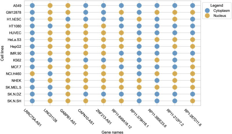 FIGURE 1
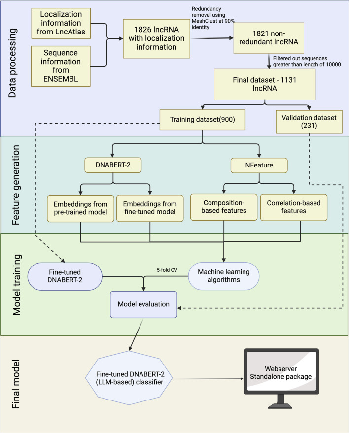 FIGURE 2
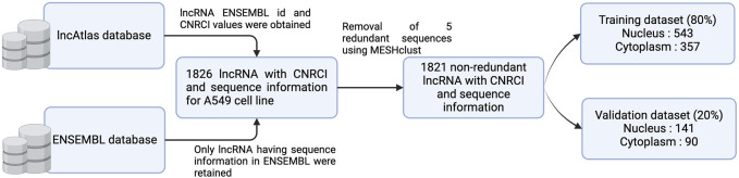 FIGURE 3
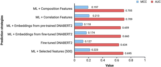 FIGURE 4
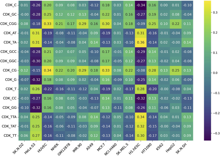 FIGURE 5
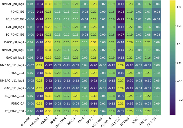 FIGURE 6
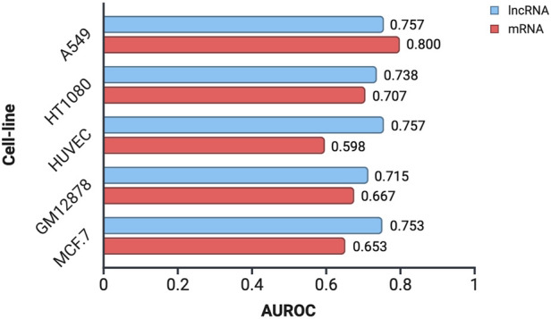 FIGURE 7
| Cell-lines | Original | Non-redundant dataset | Filtering out sequences >10,000 length | Training dataset (complete) | Training dataset (nucleus) | Training dataset (cytoplasm) | Validation dataset (complete) | Validation dataset (nucleus) | Validation dataset (cytoplasm) |
|---|---|---|---|---|---|---|---|---|---|
| 1826 | 1821 | 1131 | 904 | 547 | 357 | 227 | 137 | 90 | |
| H1.hESC | 4194 | 4178 | 2552 | 2041 | 1224 | 817 | 511 | 307 | 204 |
| HeLa.S3 | 1142 | 1141 | 703 | 562 | 470 | 92 | 141 | 118 | 23 |
| HepG2 | 1703 | 1699 | 1029 | 823 | 598 | 225 | 206 | 150 | 56 |
| HT1080 | 1183 | 1180 | 690 | 552 | 314 | 238 | 138 | 78 | 60 |
| HUVEC | 1870 | 1859 | 1137 | 909 | 659 | 250 | 228 | 165 | 63 |
| MCF.7 | 2714 | 2703 | 1702 | 1361 | 1028 | 333 | 341 | 257 | 84 |
| NCI.H460 | 772 | 769 | 460 | 368 | 304 | 64 | 92 | 76 | 16 |
| NHEK | 1383 | 1378 | 755 | 604 | 450 | 154 | 151 | 112 | 39 |
| SK.MEL.5 | 694 | 691 | 380 | 304 | 242 | 62 | 76 | 60 | 16 |
| SK.N.DZ | 762 | 759 | 422 | 337 | 205 | 132 | 85 | 52 | 33 |
| SK.N.SH | 2086 | 2077 | 1211 | 968 | 715 | 253 | 243 | 179 | 64 |
| GM12878 | 2136 | 2128 | 1286 | 1028 | 788 | 240 | 258 | 198 | 60 |
| K562 | 1197 | 1191 | 729 | 583 | 414 | 169 | 146 | 104 | 42 |
| IMR.90 | 497 | 496 | 314 | 251 | 133 | 118 | 63 | 34 | 29 |
| Feature name | Type of descriptor | No. of descriptors |
|---|---|---|
| Nucleic acid Composition | Di-Nucleotide | 16 |
| Reverse complement K-Mer composition | Di-Nucleotide | 10 |
| Nucleotide Repeat Index | Mono-Nucleotide | 4 |
| Entropy | Sequence-level | 1 |
| Entropy | Nucleotide-level | 4 |
| Distance Distribution | Mono-Nucleotide | 4 |
| Pseudo Composition | Pseudo Di-nucleotide | 19 |
| Pseudo Composition | Pseudo Tri-nucleotide | 65 |
| Total number of descriptors | 123 |
| Feature name | Type of descriptor | Number of descriptors |
|---|---|---|
| Cross Correlation | Trinucleotide Cross Correlation | 264 |
| Auto-Cross Correlation | Auto Dinucleotide - Cross Correlation | 288 |
| Auto-Cross Correlation | Auto Trinucleotide - Cross Correlation | 288 |
| Auto Correlation | Tri-Nucleotide | 24 |
| Auto Correlation | Normalized Moreau-Broto | 24 |
| Auto Correlation | Dinucleotide Moran | 24 |
| Auto Correlation | Dinucleotide Geary | 24 |
| Pseudo Correlation | Serial Correlation Pseudo Trinucleotide Composition | 65 |
| Pseudo Correlation | Serial Correlation Pseudo Dinucleotide Composition | 17 |
| Pseudo Correlation | Parallel Correlation Pseudo Trinucleotide Composition | 65 |
| Pseudo Correlation | Parallel Correlation Pseudo Dinucleotide Composition | 17 |
| Total number of descriptors | 1100 |
| Top 5 positively correlated features | Top 5 negatively correlated features | |||||||||
|---|---|---|---|---|---|---|---|---|---|---|
| SK.N.DZ | CDK_CGA | CDK_TCG | CDK_AAC | CDK_ACG | CDK_CG | CDK_TGG | CDK_TG | CDK_CTG | CDK_GGG | CDK_GGT |
| HeLa.S3 | CDK_TAC | CDK_AA | CDK_AAT | CDK_A | CDK_TA | CDK_GG | CDK_G | CDK_GGG | CDK_GGC | CDK_CTG |
| HUVEC | CDK_CG | CDK_GCG | CDK_CGG | CDK_CGA | CDK_CGC | CDK_TG | CDK_CAT | CDK_T | CDK_TGA | CDK_ATG |
| NHEK | CDK_GCG | CDK_CGC | CDK_CCG | CDK_CG | CDK_CGG | CDK_TG | CDK_TGT | CDK_GTG | CDK_GT | CDK_TCT |
| GM12878 | CDK_CGA | CDK_ACG | CDK_CG | CDK_GCG | CDK_TCG | CDK_CAT | CDK_TCA | CDK_TAT | CDK_AT | CDK_TTC |
| IMR.90 | CDK_CGA | CDK_GCG | CDK_CG | CDK_CGG | CDK_CGC | CDK_TG | CDK_TGG | CDK_CTG | CDK_CCT | CDK_CT |
| A549 | CDK_CGA | CDK_AAA | CDK_AA | CDK_GCG | CDK_GAA | CDK_CTG | CDK_CA | CDK_CAG | CDK_TG | CDK_CCA |
| MCF.7 | CDK_CGA | CDK_CG | CDK_GCG | CDK_CGC | CDK_CGG | CDK_TG | CDK_ATG | CDK_CAT | CDK_TGT | CDK_T |
| NCI.H460 | CDK_AAC | CDK_CGA | CDK_CAA | CDK_ACG | CDK_CGT | CDK_TGG | CDK_TG | CDK_GGG | CDK_GTG | CDK_GGT |
| SK.MEL.5 | CDK_CGC | CDK_CG | CDK_CCG | CDK_ACG | CDK_CGA | CDK_AGT | CDK_GAT | CDK_TGA | CDK_TG | CDK_TTG |
| H1.hESC | CDK_TA | CDK_TTA | CDK_TAA | CDK_AAT | CDK_AA | CDK_CTG | CDK_CAG | CDK_C | CDK_CCA | CDK_CC |
| HT1080 | CDK_CGA | CDK_CG | CDK_GCG | CDK_ACG | CDK_CGC | CDK_TG | CDK_T | CDK_ATG | CDK_TGT | CDK_TTT |
| K562 | CDK_CGA | CDK_CG | CDK_GCG | CDK_ACG | CDK_CGC | CDK_CAG | CDK_AG | CDK_CTG | CDK_TGG | CDK_CA |
| HepG2 | CDK_CGA | CDK_CG | CDK_TCG | CDK_GCG | CDK_CGC | CDK_TG | CDK_CT | CDK_CTG | CDK_CA | CDK_TGT |
| SK.N.SH | CDK_AA | CDK_AAC | CDK_AAA | CDK_TAA | CDK_CAA | CDK_CTG | CDK_TG | CDK_TGG | CDK_CAG | CDK_CCA |
| Top 5 positively correlated features | Top 5 negatively correlated features | |||||||||
|---|---|---|---|---|---|---|---|---|---|---|
| SK.N.DZ | TCC_p3_p4_lag1 | TACC_p3_p4_lag1 | TCC_p3_p11_lag1 | TACC_p3_p11_lag1 | TCC_p2_p3_lag2 | DACC_p1_p4_lag1 | TCC_p3_p12_lag1 | TACC_p3_p12_lag1 | TCC_p12_p3_lag1 | TACC_p12_p3_lag1 |
| HeLa.S3 | DACC_p5_p3_lag1 | PC_PTNC_TAG | SC_PTNC_TAG | PKNC_TAG | TAC_p1_lag1 | TCC_p1_p8_lag1 | TACC_p1_p8_lag1 | TCC_p8_p1_lag1 | TACC_p8_p1_lag1 | TCC_p2_p8_lag1 |
| HUVEC | DACC_p7_lag1 | DACC_p9_p8_lag1 | DACC_p1_p7_lag1 | DACC_p4_p2_lag1 | DACC_p4_p8_lag1 | DACC_p9_p7_lag1 | DACC_p1_p8_lag1 | DACC_p4_p7_lag1 | DACC_p7_p2_lag1 | DACC_p7_p4_lag1 |
| NHEK | DACC_p4_p2_lag1 | DACC_p10_p2_lag1 | DACC_p6_p2_lag1 | DACC_p7_p12_lag1 | DACC_p9_p4_lag1 | DACC_p7_p2_lag1 | DACC_p4_p12_lag1 | DACC_p6_p12_lag1 | DACC_p9_p7_lag1 | PC_PDNC_TT |
| GM12878 | TCC_p9_p3_lag1 | TCC_p10_p3_lag1 | TACC_p9_p3_lag1 | TACC_p10_p3_lag1 | TCC_p3_p9_lag1 | DACC_p9_p7_lag1 | DACC_p4_p7_lag1 | DACC_p7_p4_lag1 | DACC_p7_p6_lag1 | DACC_p6_p7_lag1 |
| IMR.90 | DACC_p4_p2_lag1 | DACC_p6_p2_lag1 | DACC_p1_p7_lag1 | DACC_p10_p2_lag1 | MAC_p2_lag1 | DACC_p6_p12_lag1 | DACC_p7_p2_lag1 | DACC_p9_p7_lag1 | DACC_p1_p2_lag1 | DACC_p4_p12_lag1 |
| A549 | DACC_p1_lag1 | DACC_p4_lag1 | DACC_p8_p9_lag2 | TAC_p3_lag1 | TACC_p3_lag1 | DACC_p9_p1_lag1 | DACC_p4_p1_lag1 | DACC_p8_p1_lag2 | DACC_p1_p4_lag1 | DACC_p7_p9_lag2 |
| MCF.7 | DACC_p7_lag1 | DACC_p1_p7_lag1 | DACC_p9_p8_lag1 | DACC_p4_p2_lag1 | DACC_p4_p8_lag1 | DACC_p1_p8_lag1 | DACC_p9_p7_lag1 | DACC_p4_p7_lag1 | DACC_p7_p2_lag1 | DACC_p7_p4_lag1 |
| NCI.H460 | DACC_p9_p4_lag1 | DACC_p1_p7_lag1 | DACC_p9_p6_lag1 | DACC_p7_p12_lag1 | DACC_p4_p6_lag1 | DACC_p1_p10_lag1 | DACC_p1_p6_lag1 | DACC_p1_p4_lag1 | DACC_p4_p12_lag1 | DACC_p10_p12_lag1 |
| SK.MEL.5 | DACC_p9_p8_lag1 | DACC_p4_p2_lag1 | DACC_p9_p2_lag1 | DACC_p10_p2_lag1 | SC_PTNC_CGG | TCC_p3_p7_lag1 | TACC_p3_p7_lag1 | DACC_p9_p7_lag1 | TCC_p7_p3_lag1 | TACC_p7_p3_lag1 |
| H1.hESC | NMBAC_p1_lag1 | DACC_p3_p11_lag1 | DACC_p1_lag1 | DACC_p3_p5_lag1 | PDNC_TC | PKNC_CTT | PKNC_CAT | SC_PTNC_CTT | PC_PTNC_CTT | SC_PTNC_CAT |
| HT1080 | DACC_p4_p2_lag1 | DACC_p1_p7_lag1 | DACC_p10_p2_lag1 | DACC_p7_lag1 | DACC_p6_p2_lag1 | DACC_p9_p7_lag1 | DACC_p1_p8_lag1 | DACC_p7_p2_lag1 | DACC_p1_p2_lag1 | DACC_p4_p7_lag1 |
| K562 | TCC_p9_p3_lag1 | TCC_p10_p3_lag1 | TACC_p9_p3_lag1 | TACC_p10_p3_lag1 | TCC_p3_p9_lag1 | DACC_p1_p8_lag2 | DACC_p1_p4_lag1 | DACC_p1_p10_lag2 | DACC_p4_p1_lag2 | DACC_p9_p7_lag2 |
| HepG2 | DACC_p7_p1_lag1 | TAC_p3_lag1 | TACC_p3_lag1 | DACC_p4_lag1 | DACC_p1_p7_lag1 | DACC_p4_p7_lag1 | DACC_p7_p4_lag1 | DACC_p7_p6_lag1 | DACC_p6_p7_lag1 | DACC_p9_p7_lag1 |
| SK.N.SH | DACC_p1_lag1 | DACC_p1_p7_lag1 | DACC_p9_p4_lag1 | DACC_p8_p9_lag2 | TCC_p11_p3_lag1 | DACC_p1_p4_lag1 | DACC_p9_p1_lag1 | DACC_p4_p1_lag1 | DACC_p1_p6_lag1 | TCC_p12_p3_lag1 |
| Cell-lines | Feature used | ML model used | Sensitivity | Specificity | Precision | Accuracy | MCC | F1-score | AUC |
|---|---|---|---|---|---|---|---|---|---|
| A549 | RDK | RandomForestClassifier | 0.600 | 0.825 | 0.692 | 0.736 | 0.438 | 0.643 | 0.761 |
| H1.hESC | CDK | RandomForestClassifier | 0.500 | 0.785 | 0.607 | 0.671 | 0.297 | 0.548 | 0.708 |
| HeLa.S3 | PKNC | GaussianNB | 0.826 | 0.593 | 0.284 | 0.631 | 0.310 | 0.422 | 0.779 |
| HepG2 | RDK | GaussianNB | 0.429 | 0.847 | 0.511 | 0.733 | 0.292 | 0.466 | 0.718 |
| HT1080 | CDK | MLPClassifier | 0.517 | 0.769 | 0.633 | 0.659 | 0.296 | 0.569 | 0.728 |
| HUVEC | PKNC | SVC | 0.032 | 0.964 | 0.250 | 0.706 | −0.011 | 0.056 | 0.756 |
| MCF.7 | CDK | GaussianNB | 0.452 | 0.809 | 0.437 | 0.721 | 0.259 | 0.444 | 0.724 |
| NCI.H460 | PKNC | SVC | 0.000 | 1.000 | 0.000 | 0.826 | 0.000 | 0.000 | 0.723 |
| NHEK | CDK | SVC | 0.000 | 1.000 | 0.000 | 0.742 | 0.000 | 0.000 | 0.643 |
| SK.MEL.5 | CDK | XGBClassifier | 0.063 | 0.950 | 0.250 | 0.763 | 0.023 | 0.100 | 0.676 |
| SK.N.DZ | CDK | MLPClassifier | 0.545 | 0.692 | 0.529 | 0.635 | 0.237 | 0.537 | 0.679 |
| SK.N.SH | PDNC | QuadraticDiscriminantAnalysis | 0.547 | 0.732 | 0.422 | 0.683 | 0.259 | 0.476 | 0.703 |
| GM12878 | PKNC | GradientBoostingClassifier | 0.133 | 0.939 | 0.400 | 0.752 | 0.115 | 0.200 | 0.687 |
| K562 | ALL_COMP | DecisionTreeClassifier | 0.452 | 0.788 | 0.463 | 0.692 | 0.243 | 0.458 | 0.620 |
| IMR.90 | PKNC | AdaBoostClassifier | 0.448 | 0.735 | 0.591 | 0.603 | 0.192 | 0.510 | 0.668 |
| Average | 0.370 | 0.829 | 0.405 | 0.704 | 0.197 | 0.362 | 0.705 |
| Cell-lines | Feature used | ML model used | Sensitivity | Specificity | Precision | Accuracy | MCC | F1-score | AUC |
|---|---|---|---|---|---|---|---|---|---|
| A549 | PC_PDNC | GradientBoostingClassifier | 0.567 | 0.803 | 0.654 | 0.709 | 0.381 | 0.607 | 0.757 |
| H1.hESC | PDNC | RandomForestClassifier | 0.495 | 0.811 | 0.635 | 0.685 | 0.324 | 0.556 | 0.720 |
| HeLa.S3 | PKNC | GaussianNB | 0.783 | 0.585 | 0.269 | 0.617 | 0.272 | 0.400 | 0.779 |
| HepG2 | MAC | GaussianNB | 0.679 | 0.567 | 0.369 | 0.597 | 0.218 | 0.478 | 0.715 |
| HT1080 | SC_PTNC | GaussianProcessClassifier | 0.583 | 0.769 | 0.660 | 0.688 | 0.359 | 0.619 | 0.738 |
| HUVEC | PDNC | AdaBoostClassifier | 0.302 | 0.897 | 0.528 | 0.732 | 0.243 | 0.384 | 0.757 |
| MCF.7 | SC_PDNC | SVC | 0.000 | 1.000 | 0.000 | 0.754 | 0.000 | 0.000 | 0.753 |
| NCI.H460 | PDNC | SVC | 0.000 | 1.000 | 0.000 | 0.826 | 0.000 | 0.000 | 0.683 |
| NHEK | PKNC | AdaBoostClassifier | 0.231 | 0.866 | 0.375 | 0.702 | 0.116 | 0.286 | 0.635 |
| SK.MEL.5 | PDNC | GradientBoostingClassifier | 0.063 | 0.933 | 0.200 | 0.750 | −0.007 | 0.095 | 0.654 |
| SK.N.DZ | TAC | SVC | 0.424 | 0.865 | 0.667 | 0.694 | 0.327 | 0.519 | 0.739 |
| SK.N.SH | PC_PTNC | GaussianNB | 0.750 | 0.531 | 0.364 | 0.588 | 0.248 | 0.490 | 0.689 |
| GM12878 | PC_PDNC | XGBClassifier | 0.350 | 0.899 | 0.512 | 0.771 | 0.288 | 0.416 | 0.715 |
| K562 | DACC | AdaBoostClassifier | 0.405 | 0.808 | 0.459 | 0.692 | 0.221 | 0.430 | 0.642 |
| IMR.90 | PC_PTNC | AdaBoostClassifier | 0.621 | 0.588 | 0.563 | 0.603 | 0.208 | 0.590 | 0.655 |
| Average | 0.417 | 0.795 | 0.417 | 0.694 | 0.213 | 0.391 | 0.709 |
| Cell-lines | ML model used | Sensitivity | Specificity | Precision | Accuracy | MCC | F1-score | AUC |
|---|---|---|---|---|---|---|---|---|
| A549 | SVC linear | 0.500 | 0.759 | 0.577 | 0.656 | 0.267 | 0.536 | 0.661 |
| H1.hESC | MLP Classifier | 0.588 | 0.638 | 0.519 | 0.618 | 0.223 | 0.552 | 0.666 |
| HeLa.S3 | XGBoost Classifier | 0.087 | 0.992 | 0.667 | 0.844 | 0.201 | 0.154 | 0.699 |
| HepG2 | MLP Classifier | 0.000 | 1.000 | 0.000 | 0.728 | 0.000 | 0.000 | 0.706 |
| HT1080 | MLP Classifier | 0.817 | 0.513 | 0.563 | 0.645 | 0.338 | 0.667 | 0.735 |
| HUVEC | Random Forest Classifier | 0.032 | 0.982 | 0.400 | 0.719 | 0.041 | 0.059 | 0.690 |
| MCF.7 | MLP Classifier | 0.012 | 0.984 | 0.200 | 0.745 | −0.013 | 0.022 | 0.657 |
| NCI.H460 | Gradient Boosting Classifier | 0.063 | 1.000 | 1.000 | 0.837 | 0.228 | 0.118 | 0.599 |
| NHEK | Gaussian Naive Bayes Classifier | 0.538 | 0.705 | 0.389 | 0.662 | 0.223 | 0.452 | 0.660 |
| SK.MEL.5 | KNN | 0.063 | 0.967 | 0.333 | 0.776 | 0.061 | 0.105 | 0.638 |
| SK.N.DZ | Gradient Boosting Classifier | 0.364 | 0.808 | 0.545 | 0.635 | 0.191 | 0.436 | 0.678 |
| SK.N.SH | MLP Classifier | 0.469 | 0.709 | 0.366 | 0.646 | 0.166 | 0.411 | 0.618 |
| GM12878 | Logistic Regression | 0.117 | 0.955 | 0.438 | 0.760 | 0.125 | 0.184 | 0.655 |
| K562 | Logistic Regression | 0.071 | 0.923 | 0.273 | 0.678 | −0.009 | 0.113 | 0.609 |
| IMR.90 | Random Forest Classifier | 0.345 | 0.824 | 0.625 | 0.603 | 0.193 | 0.444 | 0.699 |
| Average | 0.271 | 0.851 | 0.460 | 0.704 | 0.149 | 0.284 | 0.665 |
| Cell-lines | ML model used | Sensitivity | Specificity | Precision | Accuracy | MCC | F1-score | AUC |
|---|---|---|---|---|---|---|---|---|
| A549 | SVC_linear | 0.489 | 0.708 | 0.524 | 0.621 | 0.200 | 0.506 | 0.660 |
| H1.hESC | SVC_linear | 0.422 | 0.801 | 0.585 | 0.650 | 0.241 | 0.490 | 0.687 |
| HeLa.S3 | MLP Classifier | 0.000 | 0.992 | 0.000 | 0.830 | −0.037 | 0.000 | 0.732 |
| HepG2 | Gaussian Naive Bayes Classifier | 0.571 | 0.767 | 0.478 | 0.714 | 0.321 | 0.520 | 0.708 |
| HT1080 | SVC_linear | 0.450 | 0.756 | 0.587 | 0.623 | 0.217 | 0.509 | 0.700 |
| HUVEC | MLP Classifier | 0.206 | 0.903 | 0.448 | 0.711 | 0.147 | 0.283 | 0.726 |
| MCF.7 | Gaussian Naive Bayes Classifier | 0.512 | 0.739 | 0.391 | 0.683 | 0.232 | 0.443 | 0.700 |
| NCI.H460 | XGBoost Classifier | 0.000 | 0.987 | 0.000 | 0.815 | −0.048 | 0.000 | 0.535 |
| NHEK | AdaBoost Classifier | 0.359 | 0.821 | 0.412 | 0.702 | 0.189 | 0.384 | 0.600 |
| SK.MEL.5 | SVC_radial | 0.000 | 1.000 | 0.000 | 0.789 | 0.000 | 0.000 | 0.539 |
| SK.N.DZ | Gradient Boosting Classifier | 0.515 | 0.692 | 0.515 | 0.624 | 0.207 | 0.515 | 0.717 |
| SK.N.SH | AdaBoost Classifier | 0.156 | 0.866 | 0.294 | 0.679 | 0.028 | 0.204 | 0.587 |
| GM12878 | Gradient Boosting Classifier | 0.183 | 0.939 | 0.478 | 0.764 | 0.182 | 0.265 | 0.683 |
| K562 | Gradient Boosting Classifier | 0.143 | 0.894 | 0.353 | 0.678 | 0.052 | 0.203 | 0.590 |
| IMR.90 | Gradient Boosting Classifier | 0.552 | 0.706 | 0.615 | 0.635 | 0.261 | 0.582 | 0.671 |
| Average | 0.304 | 0.838 | 0.379 | 0.701 | 0.146 | 0.327 | 0.656 |
| Cell-lines | Sensitivity | Specificity | Precision | Accuracy | MCC | F1-score | AUC |
|---|---|---|---|---|---|---|---|
| A549 | 0.500 | 0.861 | 0.703 | 0.718 | 0.393 | 0.584 | 0.762 |
| H1.hESC | 0.520 | 0.713 | 0.546 | 0.636 | 0.235 | 0.533 | 0.644 |
| HeLa.S3 | 0.000 | 1.000 | 0.000 | 0.837 | 0.000 | 0.000 | 0.527 |
| HepG2 | 0.000 | 1.000 | 0.000 | 0.728 | 0.000 | 0.000 | 0.698 |
| HT1080 | 0.567 | 0.731 | 0.618 | 0.659 | 0.301 | 0.591 | 0.676 |
| HUVEC | 0.159 | 0.976 | 0.714 | 0.750 | 0.251 | 0.260 | 0.710 |
| MCF.7 | 0.000 | 1.000 | 0.000 | 0.754 | 0.000 | 0.000 | 0.562 |
| NCI.H460 | 0.000 | 1.000 | 0.000 | 0.826 | 0.000 | 0.000 | 0.576 |
| NHEK | 0.000 | 1.000 | 0.000 | 0.742 | 0.000 | 0.000 | 0.564 |
| SK.MEL.5 | 0.000 | 1.000 | 0.000 | 0.789 | 0.000 | 0.000 | 0.468 |
| SK.N.DZ | 0.515 | 0.885 | 0.739 | 0.741 | 0.439 | 0.607 | 0.791 |
| SK.N.SH | 0.000 | 1.000 | 0.000 | 0.737 | 0.000 | 0.000 | 0.589 |
| GM12878 | 0.000 | 1.000 | 0.000 | 0.767 | 0.000 | 0.000 | 0.718 |
| K562 | 0.190 | 0.885 | 0.400 | 0.685 | 0.099 | 0.258 | 0.570 |
| IMR.90 | 0.655 | 0.529 | 0.543 | 0.587 | 0.185 | 0.594 | 0.649 |
| Average | 0.207 | 0.905 | 0.284 | 0.730 | 0.127 | 0.228 | 0.634 |
| Cell lines | Top 10 | Top 50 | Top 100 | Top 500 | Top 1000 | Top 1500 | Top 2000 |
|---|---|---|---|---|---|---|---|
| A549 | 0.756 | 0.75 | 0.749 | 0.741 | 0.739 | 0.738 | 0.738 |
| GM12878 | 0.725 | 0.706 | 0.706 | 0.727 | 0.742 | 0.734 | 0.719 |
| H1.hESC | 0.677 | 0.687 | 0.694 | 0.71 | 0.712 | 0.716 | 0.717 |
| HT1080 | 0.71 | 0.73 | 0.728 | 0.731 | 0.745 | 0.749 | 0.742 |
| HUVEC | 0.733 | 0.744 | 0.762 | 0.771 | 0.76 | 0.748 | 0.764 |
| HeLa.S3 | 0.669 | 0.728 | 0.756 | 0.734 | 0.718 | 0.776 | 0.779 |
| HepG2 | 0.736 | 0.722 | 0.725 | 0.72 | 0.691 | 0.673 | 0.685 |
| IMR.90 | 0.725 | 0.651 | 0.647 | 0.621 | 0.636 | 0.602 | 0.663 |
| K562 | 0.615 | 0.665 | 0.645 | 0.628 | 0.585 | 0.581 | 0.586 |
| MCF.7 | 0.706 | 0.728 | 0.73 | 0.701 | 0.715 | 0.721 | 0.711 |
| NCI.H460 | 0.535 | 0.514 | 0.533 | 0.638 | 0.553 | 0.593 | 0.568 |
| NHEK | 0.64 | 0.634 | 0.626 | 0.609 | 0.603 | 0.632 | 0.65 |
| SK.MEL.5 | 0.672 | 0.652 | 0.552 | 0.725 | 0.597 | 0.619 | 0.575 |
| SK.N.DZ | 0.671 | 0.664 | 0.675 | 0.704 | 0.705 | 0.715 | 0.707 |
| SK.N.SH | 0.683 | 0.684 | 0.685 | 0.669 | 0.683 | 0.684 | 0.682 |
| Average | 0.683 | 0.684 | 0.681 | 0.695 | 0.679 | 0.685 | 0.686 |
| lncLocator 2.0 | TACOS | CytoLncPred – Composition features | CytoLncPred – Correlation features | |
|---|---|---|---|---|
| A549 | 0.592 | 0.741 | 0.761 | 0.757 |
| H1.hESC | 0.649 | 0.752 | 0.708 | 0.720 |
| HeLa.S3 | 0.492 | 0.721 | 0.779 | 0.779 |
| HepG2 | 0.487 | 0.712 | 0.718 | 0.715 |
| HT1080 | 0.597 | 0.727 | 0.728 | 0.738 |
| HUVEC | 0.500 | 0.721 | 0.756 | 0.757 |
| MCF.7 | 0.530 | - | 0.724 | 0.753 |
| NCI.H460 | 0.500 | - | 0.723 | 0.683 |
| NHEK | 0.519 | 0.623 | 0.643 | 0.635 |
| SK.MEL.5 | 0.500 | 0.567 | 0.676 | 0.654 |
| SK.N.DZ | 0.500 | - | 0.679 | 0.739 |
| SK.N.SH | 0.508 | 0.633 | 0.703 | 0.689 |
| GM12878 | 0.500 | 0.568 | 0.687 | 0.715 |
| K562 | 0.500 | - | 0.620 | 0.642 |
| IMR.90 | 0.471 | - | 0.668 | 0.655 |
| Average | 0.523 | 0.676 | 0.705 | 0.709 |
Peer Reviews
No public reviews on file for this paper yet. If you reviewed it on a platform where reviews are public (OpenReview, ICLR, NeurIPS, ICML), you can paste yours below so the community can read it here.
Videos
No videos yet. Explain this paper in a talk, walkthrough, or lecture? Add one.
Taxonomy
TopicsCancer-related molecular mechanisms research · Plant and Fungal Interactions Research · Genomics and Phylogenetic Studies
Highlights
• Prediction of cytoplasm-associated lncRNAs in 15 human cell lines
• Machine learning using composition and correlation features
• DNABERT-2 embeddings for lncRNA localization prediction
• Correlation-based models outperform LLM-based models
• Web server and models available for public use
Introduction
The rapidly expanding field of non-coding RNAs has revolutionized our understanding of gene regulation and cell biology. Among the diverse classes of non-coding RNAs, long non-coding RNAs (lncRNAs) have attracted significant attention due to their ability to regulate gene expression at various levels. Initially dismissed as transcriptional noise, lncRNAs have emerged as critical players in cellular processes, including development, differentiation, and disease progression (Statello et al., 2021). To fully comprehend the functional roles of lncRNAs, it is imperative to investigate their subcellular localization. lncRNAs have distinct functions in the nucleus and cytoplasm, influencing transcriptional and posttranscriptional processes. In the nucleus, lncRNAs regulate gene expression and chromatin organization, while in the cytoplasm, they participate in signal transduction and translation. Some lncRNAs exhibit dual localization and functional diversification, reflecting their adaptability to different subcellular environments (Miao et al., 2019; Aillaud and Schulte, 2020; Mattick et al., 2023).
In recent years, extensive research efforts have been focused on deciphering the subcellular localization of lncRNAs. Various experimental approaches, such as fluorescence in situ hybridization (FISH) (Chang et al., 2023), RNA sequencing (RNA-seq) (Mayer and Churchman, 2017), and fractionation techniques (Miao et al., 2019), have been employed to identify the subcellular localization patterns of lncRNAs. These studies have revealed that lncRNAs can be localized in different cellular compartments, including the nucleus, cytoplasm, nucleolus, and specific subcellular structures. The subcellular localization of lncRNAs is often associated with their biological functions. For instance, nuclear-localized lncRNAs are frequently involved in transcriptional regulation, chromatin remodeling, and epigenetic modifications. Cytoplasmic lncRNAs, on the other hand, can interact with proteins or act as competitive endogenous RNAs (ceRNAs) to regulate gene expression post-transcriptionally (Bridges et al., 2021). However, most of these methods are expensive to perform and require highly specialized instrumentation.
Advancements in computational methods and machine learning approaches have further facilitated the prediction of lncRNA subcellular localization. These methods leverage various features, such as sequence composition, secondary structure, and evolutionary conservation, to predict the subcellular localization of lncRNAs with high accuracy. Several computational methods have been proposed for predicting lncRNA subcellular localization. Sequence-based methods rely on the nucleotide composition of the lncRNA. They utilize features such as k-mer frequency, nucleotide composition, and sequence motifs. However, these methods are trained on datasets that are not unique to humans, and they do not account for the variation in the subcellular localization of lncRNA in different cells.
Cell-line specific subcellular localization gains prominence due to the variability (in terms of subcellular localization) that lncRNAs exhibit within different cell-lines. This was reported by Lin et al. in lncLocator 2.0, where it was observed that a single lncRNA had different localization in different cell-lines (Lin et al., 2021). We observed a similar trend in our dataset, where some lncRNAs were found to be localized in the nucleus for some cell-lines but were localizing to the cytoplasm in some other cell-lines. This pattern can be seen clearly in Figure 1.
Bubble plot indicating the variability of localization of a single lncRNA across multiple cell-lines.
lncLocator 2.0 is a cell-line-specific subcellular localization predictor that employs an interpretable deep-learning approach (Lin et al., 2021). TACOS, also a cell-line-specific subcellular localization predictor, uses tree-based algorithms along with various sequence compositional and physicochemical features (Jeon et al., 2022). Among all the existing computational methods, only lncLocator 2.0 and TACOS are designed to predict subcellular localization specific to different cell-lines. The primary issue with these methods is that the datasets used to develop these methods have not been properly filtered. Specifically, these methods have included mRNA sequences in their datasets, which can lead to inaccurate predictions. Additionally, the datasets have eliminated lncRNAs with an absolute fold-change less than 2, which can result in the failure to predict the subcellular location of lncRNAs with borderline concentration differences between locations.
To address the limitations of existing methods in a comprehensive manner, we have developed CytoLNCpred. In this study, we aimed to enhance the prediction accuracy compared to current tools, which have significant room for improvement. Furthermore, we have cleaned the dataset and adhered to industry standards to validate the performance of our method. In CytoLNCpred, a machine learning model trained using correlation-based features demonstrated significantly better performance on the validation dataset compared to existing tools.
Materials and methods
To aid in the development of a prediction model for lncRNA subcellular localization, we’ve designed a workflow diagram, depicted in Figure 2. The comprehensive details of each phase in this workflow are outlined in the subsequent sections.
Overall architecture of CytoLNCpred.
Dataset creation
In this study, we have selected lncAtlas for acquiring cell-line specific subcellular localization information. lncAtlas is a comprehensive resource of lncRNA localization in human cells based on RNA-sequencing data sets (Mas-Ponte et al., 2017). lncAtlas contains a wide array of information, including Cytoplasm to Nucleus Relative Concentration Index (CNRCI), which we have utilized in our method. CNRCI is defined as the log2-transformed ratio of RPKM (Reads Per Kilobase per Million mapped reads) in two samples, in this case - the cytoplasm and nucleus. It is calculated as follows
Sequence information for the lncRNAs was obtained from ENSEMBL database (version 112) and lncRNAs with no sequence were dropped. In order to modify the dataset for a classification problem, we assigned sequences having CNRCI value greater than 0 as Cytoplasm and those having CNRCI value less than 0 were assigned as Nucleus. Redundancy was removed using MeshClust (Girgis, 2022), using a sequence similarity of 90%. Figure 3 graphically depicts how the training and validation datasets were created.
Graphical overview of the process of dataset creation.
Further, we used sequences up to the length of 10,000 nucleotides only, as the longer lncRNA were misleading for the machine learning models and computationally very expensive when large language models were involved. The summary of the dataset used for each cell line is provided in Table 1.
Feature generation - Composition and correlation-based
For facilitating the training of machine learning (ML) models, we generated a large variety of features using different approaches. These features convert nucleotide sequences We used the in-house tool Nfeature (Mathur et al., 2021) for generating multiple composition and correlation features.
Composition-based
Nucleotide composition-based features refer to quantitative representations of sequences that can be derived from the proportions and arrangements of nucleotides within these sequences. In this study, we have computed nucleic acid composition, distance distribution of nucleotides (DDN), nucleotide repeat index (NRI), pseudo composition and entropy of a sequence. The details for each of the features are provided in Table 2.
Correlation-based features
In this study, using Nfeature, we quantitatively assess the interdependent characteristics inherent in nucleotide sequences through the computation of correlation-based metrics. Correlation refers to the degree of relationship between distinct properties or features; an autocorrelation denotes the association of a feature with itself, whereas a cross-correlation indicates a linkage between two separate features. By employing these correlation-based descriptors, we effectively normalize the variable-length nucleotide sequences into uniform-length vectors, rendering them amenable to analysis via machine learning algorithms. These specific descriptors facilitate the identification and extraction of significant features predicated upon the nucleotide properties distributed throughout the sequence, enabling a more robust understanding of genetic information. A brief description of the features has been provided in Table 3.
The total number of descriptors generated by using both composition and correlation-based features is 1223. Detailed explanation of the features and their biological implication have been provided in Supplementary Table S1. The properties used to calculate correlation-based features are provided in Supplementary Table S2.
Embedding using DNABERT-2
DNABERT-2 is an adaptation of BERT (Bidirectional Encoder Representations from Transformers) designed specifically for DNA sequence analysis (Zhou et al., 2023). DNABERT-2 generates embeddings for DNA sequences that encapsulate not just the individual bases, but also their biological significance in terms of structure, function, and interactions. Moreover, the key advantage of DNABERT-2 embeddings lies in their ability to capture the complex dependencies within DNA sequences. We have made use of both aspects of DNABERT-2 - the pre-trained model to make predictions and the embeddings from the model to be used as features for downstream tasks. The pre-trained model was trained on the training dataset using the default parameters mentioned in their GitHub repository. Moreover, we have also generated embeddings from both the pre-trained as well as the fine-tuned models in order to use them as features for machine learning algorithms. The embeddings are derived from the hidden states of the model’s final output layer, using max pooling. The number of embeddings generated for each lncRNA using DNABERT-2 was 768.
Five-fold cross validation
In order to estimate the performance of machine learning based models while training, we have deployed five-fold cross validation. In this method, the training dataset is split into five folds in a stratified manner and training is actually done over four folds and one fold is dedicated for validation. This process is iteratively performed for five times, by changing the fold that is used for validation and the rest of the folds being used for training. This generates an unbiased set of five performance metrics and the performance of the model is reported as the mean of these five sets.
Feature selection
To optimize model performance and reduce computational complexity, we employed the Minimum Redundancy Maximum Relevance (mRMR) feature selection algorithm to identify the most informative features from our dataset. The mRMR algorithm selects features that exhibit the highest relevance to the target variable while minimizing redundancy among the features themselves, thereby enhancing the efficiency and predictive power of the models. For applying the mRMR algorithm, we combined all the features that were generated previously. Three different feature sets–Composition, Correlation and Embeddings, were used to generate a combined feature set comprising 2278 features. We evaluated the impact of feature selection by calculating and selecting subsets of 10, 50, 100, 500, 1000, 1500, and 2000 features. These subsets were subsequently used in downstream analyses to assess their influence on model performance metrics. Feature importance was also evaluated using simple correlation.
Model development
In this study, three different approaches were followed for model development. The first approach involves the fine tuning of the DNABERT-2 using our training dataset and subsequently using the fine-tuned model to make predictions on the validation dataset. This method initially fine-tunes both the tokenizer and the pre-trained model according to our training dataset, and generates a fine-tuned tokenizer, and model. The fine-tuned model takes lncRNA sequences and generates the prediction using the tokenizer and model. In the next approach, we have implemented a hybrid approach, combining the components of large language models and machine learning algorithms. Instead of features, we have generated embeddings from a pre-trained as well as fine-tuned DNABERT-2 model. Embeddings from the DNABERT-2 model were then used to train machine learning models and subsequently evaluated them. The third approach involves composition and correlation-based features and using them to train machine learning models. The final model was developed using the.
Model evaluation metrics
The binary classification performance of our fine-tuned model was evaluated using the following metrics: Sensitivity (SENS), Specificity (SPEC), Precision (PREC), Accuracy (ACC), Matthew’s Correlation Coefficient (MCC), F1-Score (F1) and Area Under the Receiver Operator Characteristic curve (AUC). The aforementioned metrics were calculated using the four different types of prediction outcomes: true positive (TP), false positive (FP), true negative (TN), and false negative (FN):
The evaluation of our binary classification model using various metrics provides critical insights into its performance. Sensitivity (SENS) measures the model’s ability to identify positive instances, while Specificity (SPEC) assesses its accuracy in recognizing negative instances. Precision (PREC) reflects the accuracy of positive predictions, and Accuracy (ACC) offers an overall measure of correctness, though it may be misleading in imbalanced datasets. Matthew’s Correlation Coefficient (MCC) provides a balanced view by considering all prediction outcomes, with values close to 1 indicating strong predictive capability. The F1-Score (F1) combines Precision and Sensitivity into a single metric, ideal for balancing the trade-off between false positives and negatives. Finally, the Area Under the Curve (AUC) evaluates the model’s ability to distinguish between classes across different thresholds, with higher values indicating better performance. Together, these metrics enable a comprehensive evaluation of the model, guiding necessary improvements and refinements.
Results
In this study, an attempt was made to design a model that will be able to classify the subcellular location of lncRNA into cytoplasm or nucleus. To achieve this, we tried out multiple approaches. Figure 4 provides an overview of the performance of the various approaches tried in this study.
Overview of the performance achieved by different prediction strategies. The values indicate the average MCC and AUC across all the 15 cell-lines for a prediction strategy.
Functional enrichment analysis
The GO and KEGG enrichment analysis, conducted using RNAenrich (Zhang et al., 2023), reveals distinct functional roles for cytoplasmic versus nuclear-localizing lncRNAs. Among the significantly enriched GO terms (adjusted p-value <0.05), 2,511 were shared, while 397 were unique to cytoplasmic lncRNAs (positive class) and 254 to nuclear lncRNAs (negative class). Cytoplasmic lncRNAs were enriched for biological processes such as “response to interferon-beta” (GO:0035456), “positive regulation of apoptotic process” (GO:0043065), and “RNA splicing” (GO:0008380), indicating roles in immune signaling, post-transcriptional regulation, and cellular stress responses. Correspondingly, KEGG pathway enrichment identified associations with Ferroptosis (hsa04216) and Autophagy (hsa04140), further highlighting their involvement in cytoplasmic stress and degradation pathways. In contrast, nuclear-localized lncRNAs were enriched for GO terms such as “eukaryotic 48S preinitiation complex” (GO:0033290), “regulation of transcription of nucleolar large rRNA by RNA polymerase I” (GO:1901836), and “MLL1/2 complex” (GO:0044665), reflecting their roles in transcriptional regulation, chromatin remodeling, and nucleolar function. KEGG analysis further linked nuclear lncRNAs to Sterol Biosynthesis (hsa00100) and Nucleotide Excision Repair (hsa03420), pointing to nuclear functions in genome maintenance and metabolic regulation. Together, these enrichments underscore the compartment-specific biological functions of lncRNAs, shaped by their cellular localization.
Feature importance
To identify features associated with subcellular localization labels (cytoplasm or nucleus), we computed the correlation of each feature with the corresponding CNRCI values. A positive correlation indicates that an increase in the feature value favors cytoplasmic localization, whereas a negative correlation suggests a preference for nuclear localization. This analysis elucidates which features predominantly influence localization to either compartment. The top 10 genes that were highly correlated with the CNRCI values are provided in Table 4, 5 for composition-based and correlation-based features, respectively. A more detailed version of this table is provided in Supplementary Table S3, 4. It can be observed that Cytosine-based k-mers are more prevalent in the positively correlated features (supporting cytoplasm localization) whereas Thymine is predominantly found in negatively correlated features (supporting nucleus localization).
Additionally, we assessed feature variability across cell lines by calculating the difference between the maximum and minimum correlation values observed for each feature across all 15 cell lines. This approach highlights features exhibiting the most pronounced inter-cell-line variation, providing insight into their potential biological or experimental variability. Figures 5, 6 represent heatmaps depicting the highly variable genes and their correlation with the CNRCI values for composition and correlation-based features, respectively. The complete information for the variable genes has been provided in Supplementary Table S5, 6.
Heatmap depicting the composition-based features that demonstrate the highest variation in their correlation with the CNRCI values within 15 cell-lines.
Heatmap depicting the correlation-based features that demonstrate the highest variation in their correlation with the CNRCI values within 15 cell-lines.
Model based on composition and correlation features
Composition and correlation features generated from Nfeature were used to train multiple ML models. We have computed the performance of nine composition-based features and thirteen correlation-based features. We implemented all the combinations of feature and ML model to identify which feature-ML model combination performs the best. The composition features combined with classical ML methods were able to achieve an average AUC of 0.7049 and a MCC of 0.1965, across the 15 cell-lines. Similarly, with correlation-based features and ML methods, the best performance achieved was an average AUC of 0.7089 and a MCC of 0.2133. Performance of the best performing model using both composition and correlation-based features are provided for all the 15 cell-lines in Table 6, 7 respectively. The detailed performance for all the models used in this analysis have been provided in Supplementary Table S7, 8. The model parameters are provided in Supplementary Table S12.
Models based on embeddings from DNABERT-2
Embeddings from large language models are known to encapsulate not just the individual bases, but also their biological significance in terms of structure, function, and interactions. In this approach, we generated high level representations of lncRNA sequences using both the pre-trained as well as the fine-tuned models. These embeddings were used to train ML models and the models were evaluated on the validation dataset. In the case of pre-trained embeddings, the model achieved an average AUC of 0.6586 and an average MCC of 0.1182. When fine-tuned embeddings were used as features, the performance of the model dropped marginally, achieving an average AUC of 0.6604 and an average MCC of 0.1740. Detailed results for the performance of ML models on the validation dataset using pre-trained as well as fine-tuned embeddings as features are provided in Table 8, 9 respectively. The detailed performance for all the models has been reported in Supplementary Table S9, 10.
Fine-tuned DNABERT-2 model
In this approach, we used our training dataset to fine-tune the model and generate a fine-tuned tokenizer and model. Using this tokenizer and model, we generate high level representations of our lncRNA sequences and these representations are used by the model to generate predictions. The fine-tuned DNABERT2 model could not be evaluated while training as we were not able to implement five-fold cross validation. The fine-tuned model was evaluated on the validation dataset and performance metrics for the same are reported in Table 10. The detailed performance for all the models has been provided in Supplementary Table S11.
Model based on features selected by mRMR algorithm
In order to identify the best set of features from the combined feature set of 2278 features (composition, correlation, and embeddings), mRMR algorithm was used. Seven different feature sets were created based on the top ‘k’ features selected by mRMR. Performance was evaluated for seven different sets of features for each cell-line using 12 different ML classifiers. Table 11 reports the AUC for the best model for each combination and the last row shows the average for each feature set. The best AUC value was reported when top 500 genes selected by mRMR was used for training.
Performance comparison of CytoLNCpred and existing state-of-the-art classifiers
To further illustrate the efficacy of our method, we conduct a comparative analysis with other cutting-edge classifiers. Specifically, we evaluate existing predictors, namely, lncLocator 2.0 and TACOS, which employ predictive algorithms to predict subcellular location of lncRNAs in different cell-lines.
Among these predictors, lncLocator 2.0 relies on the word embeddings and a MultiLayer Perceptron Regressor to predict CNRCI values. The predicted CNRCI values were then converted to labels using a fixed threshold value. The second predictor, TACOS, generated a variety of feature encodings using composition and physicochemical properties and tree-based algorithms were deployed to make the predictions. It is important to note that TACOS has been trained on 10 out of the 15 cell-lines. For a fair performance comparison, we leverage the performance metrics of evaluated on the validation dataset. Table 12 summarizes the evaluation of CytoLNCpred and other existing tools based on AUROC.
mRNA localization prediction accuracy using CytoLNCpred
To assess the applicability of CytoLNCpred, a tool originally developed for lncRNA localization prediction, to mRNA sequences, we utilized mRNA data obtained from the lncAtlas database. These mRNA sequences were subjected to prediction using the standalone version of CytoLNCpred, and its performance was evaluated using the Area Under the Receiver Operating Characteristic curve (AUROC). The AUROC values obtained for mRNA localization prediction across different cell lines, alongside the corresponding performance for lncRNA prediction, are presented in Figure 7.
Performance evaluation of CytoLNCpred in predicting the subcellular localization of mRNA and lncRNA sequences in various cell lines, as measured by the Area Under the Receiver Operating Characteristic curve (AUROC).
The results indicate that CytoLNCpred exhibits a varying degree of accuracy in predicting the subcellular localization of mRNA sequences across the tested cell lines. As illustrated in Figure 7, the predictive performance for mRNA localization differs depending on the cellular context. Notably, the highest prediction accuracy for mRNA was observed in the A549 cell line (AUROC = 0.800), suggesting a strong potential for the tool in this specific context. While the performance varied across different cell lines, with HUVEC showing the lowest AUROC (0.598), the overall results suggest that features learned by CytoLNCpred for lncRNA localization can also provide some discriminatory power for mRNA localization. Interestingly, in the A549 cell line, the prediction accuracy for mRNA even surpassed that observed for lncRNAs. However, in other cell lines like HUVEC and MCF-7, the performance on mRNA was notably lower compared to lncRNAs.
In order to further validate the model accuracy for mRNAs, 10 random cytoplasmic mRNAs were obtained from NCBI gene database. These mRNAs were then predicted using CytoLNCpred for the A549 cell-line. The model was able to predict only 2 mRNAs correctly, among the 10 cytoplasmic RNA and the detailed results are provided in Supplementary Table S13. This variability in performance across cell types highlights the potential influence of cell-specific factors on mRNA localization and suggests that further refinement or specialized models might be beneficial for broader applicability to mRNA.
Discussion
In recent years, researchers have recognized that the subcellular localization of lncRNAs plays a pivotal role in understanding their function. Unlike protein-coding genes, lncRNAs do not encode proteins directly. Instead, they exert their effects through diverse mechanisms, including interactions with chromatin, RNA molecules, and proteins. The precise localization of lncRNAs within the cell provides crucial information about their regulatory roles.
In our analysis LINC00852 showed a marked cell-line–specific shift–predominantly nuclear (negative localization score) in most cell types, but strongly cytoplasmic in the NCI-H460 lung carcinoma line. This mirrors literature reports that LINC00852 can be cytoplasmically enriched in lung carcinoma cases. In lung carcinoma cell-lines (A549 and SPCA-1), LINC00852 was found mainly in the cytoplasm (qRT-PCR assay) (Liu et al., 2018). It binds with the S100A9 protein in the cytoplasm, activating the MAPK pathway and plays a positive role in the progression and metastasis of lung adenocarcinoma cells. By contrast, other studies have observed LINC00852 in the nucleus in some tumors. In osteosarcoma cell-lines (like 143B and MG-63), it is observed that LINC00852 acts as a transcription factor and increase the expression of AXL gene (Li et al., 2020). Such context dependence could reflect tissue-specific expression of RNA-binding factors or isoforms that govern nuclear export. The fact that LINC00852 is cytoplasmic in some cancer lines but nuclear in others suggests it may switch roles-in cytosolic form it may acts as a post-transcriptional regulator (e.g., miRNA sponge), whereas nuclear retention may imply transcriptional or chromatin-related roles.
SNHG3 in our data is mostly cytoplasmic in H1.hESC, HepG2 (liver carcinoma) and GM12878 (lymphoblast) cells, but nuclear in cell-lines like MCF-7 and NHEK. This pattern aligns with experimental studies. In colorectal cancer cell lines (e.g., SW480, LoVo), SNHG3 was found to localize predominantly in the cytoplasm (comparable to GAPDH) (Huang et al., 2017). There it acts as a competing endogenous RNA (ceRNA), sponging miRNAs (e.g., miR-182-5p) to upregulate oncogenic targets like c-Myc. The high cytoplasmic SNHG3 expression in stem-cell like and proliferative cell-lines (H1.hESC, HepG2) from our dataset suggests a similar ceRNA role, whereas its nuclear enrichment in more differentiated/epithelial cells may reflect downregulation of this pathway in those contexts. In general, SNHG-family lncRNAs are known to influence cancer cell growth and often operate via cytoplasmic post-transcriptional mechanisms, consistent with SNHG3’s localization and function in promoting malignancy.
Subcellular localization of lncRNA gains prominence in recent times due to their role in gene regulation within the cell. A large number of aptamer and ASO based drugs are being developed using RNA nanotechnology. In recent years, the convergence of nanotechnology and long non-coding RNAs (lncRNAs) has yielded exciting developments in drug development. Nanoparticles, such as liposomes and exosomes, are being harnessed for targeted delivery of lncRNA-based therapeutics to cancer cells. Additionally, CRISPR-Cas9 technology, delivered via nanoparticles, enables precise gene editing by modulating lncRNA expression. Computational models and deep learning approaches are aiding our understanding of lncRNA-mediated mechanisms. Overall, this interdisciplinary field holds immense promise for personalized medicine, improved therapies, and better patient outcomes.
Predicting lncRNA subcellular localization using tools like CytoLNCpred offers significant potential for guiding the development of RNA-based therapeutics and CRISPR strategies. Since antisense oligonucleotides (ASOs) are generally more effective against nuclear lncRNAs (Zong et al., 2015) and small interfering RNAs (siRNAs) excel against cytoplasmic targets (Lennox and Behlke, 2016), a CytoLNCpred prediction indicating cytoplasmic enrichment would favor siRNA development, while a predicted nuclear localization would suggest ASOs as the primary choice. Similarly, this prediction informs CRISPR approaches: targeting nuclear-acting lncRNAs might be best achieved by disrupting transcription or key regulatory elements using CRISPRi or Cas9 (Rosenlund et al., 2021), whereas lncRNAs predicted to function in the cytoplasm could be more effectively targeted by degrading the transcript directly using RNA-targeting CRISPR-Cas13 (Xu et al., 2020), potentially guiding crRNA expression strategies (e.g., using a U1 promoter for cytoplasmic crRNA localization). Thus, localization prediction aids in the rational selection of therapeutic modalities and CRISPR targeting strategies based on the likely site of lncRNA function.
In recent times large language models are considered as SOTA methods and apart from the classical composition and correlation feature-based model, we also implemented DNABERT-2 for our classification problem. The DNABERT-2 model has been trained on the genomes of a wide variety of species and is computationally very efficient. DNABERT-2 uses Byte Pair Encoding to generate tokens which is known to perform better than k-mer tokenization. So, in order to fully exploit the DNABERT-2 model, we generated embeddings from both pre-trained and fine-tuned models. These embeddings when combined with ML methods were able to predict subcellular localization very well but poorer than a fine-tuned DNABERT-2 model.
In our study, we compared the performance of DNABERT-2 with traditional composition and correlation-based features for classifying subcellular localization of lncRNAs. While DNABERT-2, a pre-trained language model, showed promising results, but we found that traditional machine learning models trained on carefully crafted composition and correlation features consistently outperformed DNABERT-2. This suggests that for this specific task, the carefully engineered features capture the relevant biological information more effectively than the general-purpose representations learned by DNABERT-2. Specifically, it was observed that the correlation-based features achieve a higher average AUC than all other approaches. However, these approaches failed when we used RNA sequences greater than 10,000 base pairs. In order to reduce the variability in nucleotide length, the sequence length was limited to 10,000 base pairs.
The lncAtlas database, while a valuable resource for lncRNA subcellular localization, has several significant limitations including its restriction to GENCODE-annotated lncRNAs and a limited set of 15 human cell lines, with detailed sub-compartment data available only for the K562 cell line. The database relies on RNA-seq data and the Relative Concentration Index (RCI), which provides relative abundance rather than absolute counts. Furthermore, lncAtlas has not been updated since 2017, making it less comprehensive and potentially outdated.
To address these limitations, future research should focus on developing techniques to improve the interpretability of DNABERT-2’s predictions. This could involve methods such as attention visualization or feature importance analysis. Furthermore, expanding the diversity of training data is essential to enhance the model’s generalizability across different biological contexts. By incorporating data from a wider range of organisms and conditions, subcellular localization prediction could become a more versatile and reliable tool for genomic analysis. In our case, correlation-based features with machine learning algorithms outperformed all other approaches. Moreover, improved machine learning algorithms are needed to be developed that can account for large variability in nucleotide lengths.
Conclusion
Understanding the subcellular localization of lncRNA can provide great insights into their function within the cell. Computational tools have recently expanded the domain of subcellular localization by the development of faster and more accurate methods. In this study, we used a variety of machine learning as well as large language models to accurately predict lncRNA subcellular localization. The implementation of large language models to tackle biological problems is gaining momentum and our study also highlights its importance. The final model used in CytoLNCpred was designed using a traditional machine learning model trained using correlation-based features. This tool will help researchers to improve the functional annotation of lncRNA and develop RNA-based therapeutics.
The reference list from the paper itself. Each links out to its DOI / PubMed record.
- 1Aillaud M.Schulte L. N. (2020). Emerging roles of long noncoding RN As in the cytoplasmic milieu. Noncoding RNA 6, 44. 10.3390/ncrna 6040044 33182489 PMC 7711603 · doi ↗ · pubmed ↗
- 2Bridges M. C.Daulagala A. C.Kourtidis A. (2021). LN Ccation: lnc RNA localization and function. J. Cell Biol. 220, e 202009045. 10.1083/jcb.202009045 33464299 PMC 7816648 · doi ↗ · pubmed ↗
- 3Chang J.Ma X.Sun X.Zhou C.Zhao P.Wang Y. (2023). RNA fluorescence in situ hybridization for long non-coding RNA localization in human osteosarcoma cells. J. Vis. Exp. 10.3791/65545 37395584 · doi ↗ · pubmed ↗
- 4Girgis H. Z. (2022). Me Sh Clust v 3.0: high-quality clustering of DNA sequences using the mean shift algorithm and alignment-free identity scores. BMC Genomics 23, 423. 10.1186/s 12864-022-08619-0 35668366 PMC 9171953 · doi ↗ · pubmed ↗
- 5Huang W.Tian Y.Dong S.Cha Y.Li J.Guo X. (2017). The long non-coding RNA SNHG 3 functions as a competing endogenous RNA to promote malignant development of colorectal cancer. Oncol. Rep. 38, 1402–1410. 10.3892/or.2017.5837 28731158 PMC 5549033 · doi ↗ · pubmed ↗
- 6Jeon Y.-J.Hasan M. M.Park H. W.Lee K. W.Manavalan B. (2022). TACOS: a novel approach for accurate prediction of cell-specific long noncoding RN As subcellular localization. Brief. Bioinform. 23, bbac 243. 10.1093/bib/bbac 243 35753698 PMC 9294414 · doi ↗ · pubmed ↗
- 7Lennox K. A.Behlke M. A. (2016). Cellular localization of long non-coding RN As affects silencing by RN Ai more than by antisense oligonucleotides. Nucleic Acids Res. 44, 863–877. 10.1093/nar/gkv 1206 26578588 PMC 4737147 · doi ↗ · pubmed ↗
- 8Li Q.Wang X.Jiang N.Xie X.Liu N.Liu J. (2020). Exosome-transmitted linc 00852 associated with receptor tyrosine kinase AXL dysregulates the proliferation and invasion of osteosarcoma. Cancer Med. 9, 6354–6366. 10.1002/cam 4.3303 32673448 PMC 7476833 · doi ↗ · pubmed ↗