Topology entropy: Enhancing graph partitioning for TAD identification and single-cell clustering
Qiushi Liang, Shengjie Zhao, Lingxi Chen, Shuai Cheng Li

TL;DR
This paper introduces a new method using topology entropy to improve the analysis of biological graphs, such as identifying TADs and clustering single-cell data.
Contribution
The paper introduces the topology entropy encoding tree and two novel methods, TEC-O and TEC-U, for graph partitioning in biological data.
Findings
Topology entropy is robust to noise and captures structural information better than existing methods.
TEC-O and TEC-U achieve the highest accuracy in TAD detection and cell clustering, respectively.
The methods provide biologically meaningful insights from Hi-C and single-cell sequencing data.
Abstract
Entropy quantifies the limits of information compression and provides a theoretical foundation for exploring complex structures in large-scale graphs. However, effective metrics are needed to capture the intricate structural details in biological graphs. In this paper, we introduce the topology entropy encoding tree to quantify the complexity of biological graphs and show that minimizing the associated entropy is equivalent to optimal graph partitioning. We develop two methods, TEC-O and TEC-U, for partitioning ordered and unordered biological graphs. TEC-O is applied to identify Topologically Associated Domains (TADs) in Hi-C contact maps, while TEC-U is used for cell clustering in single-cell sequencing data. Results from simulated datasets demonstrate that topology entropy is robust to noise and effectively captures structural information, outperforming existing methods. Experiments…
Genes, proteins, chemicals, diseases, species, mutations and cell lines named across the full text — each resolved to its canonical identifier and authoritative record.
Click any figure to enlarge with its caption.
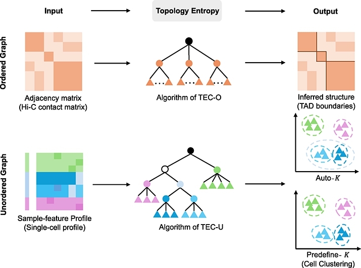 Figure 1
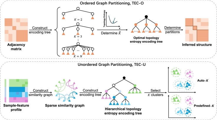 Figure 2
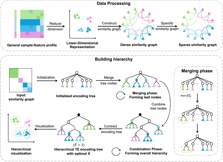 Figure 3
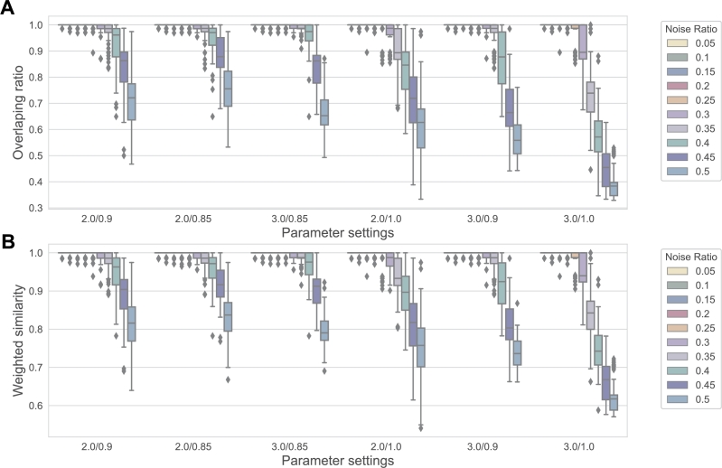 Figure 4
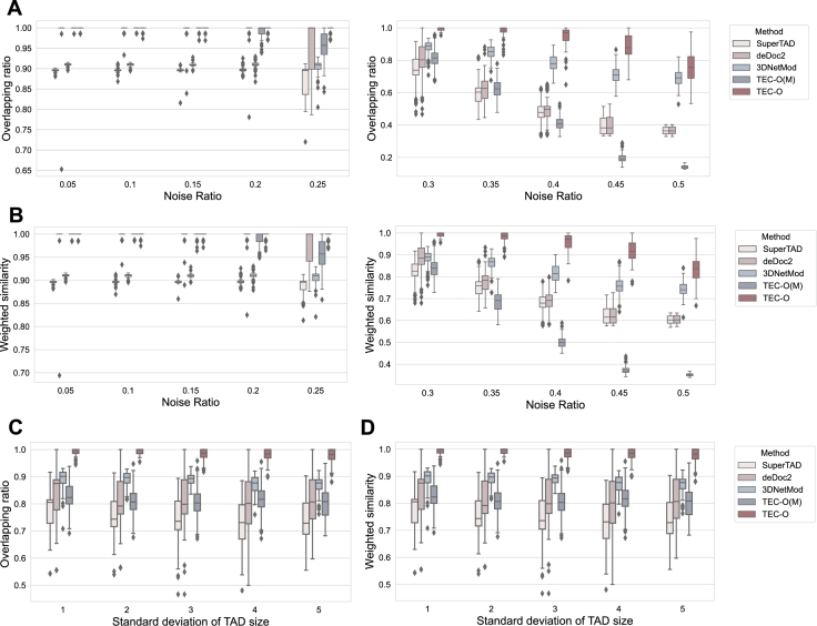 Figure 5
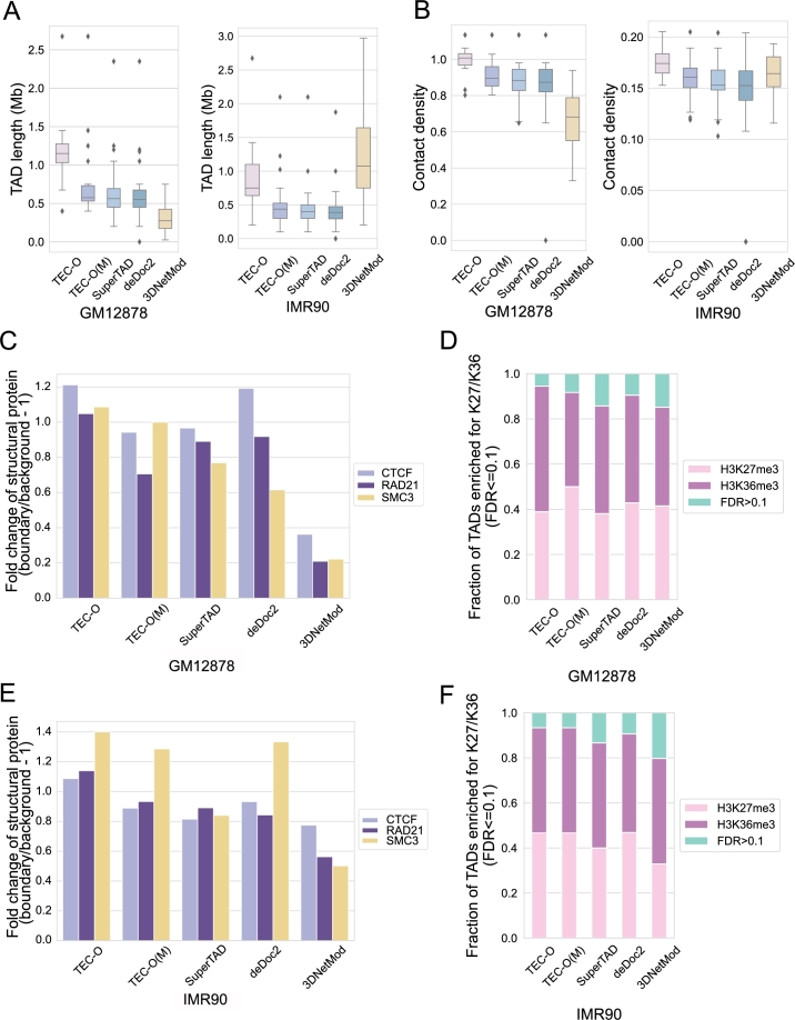 Figure 6
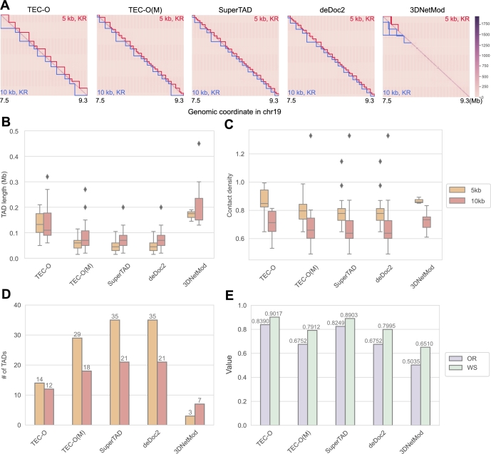 Figure 7
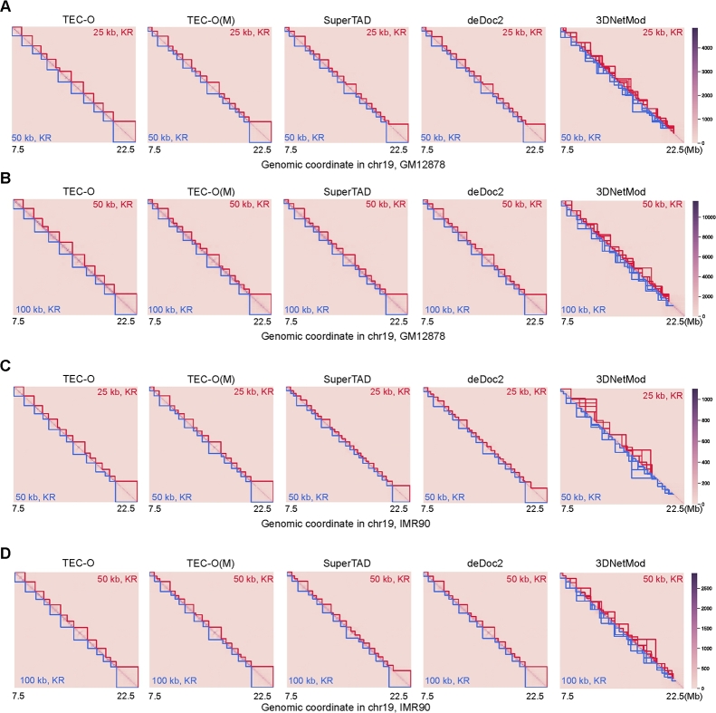 Figure 8
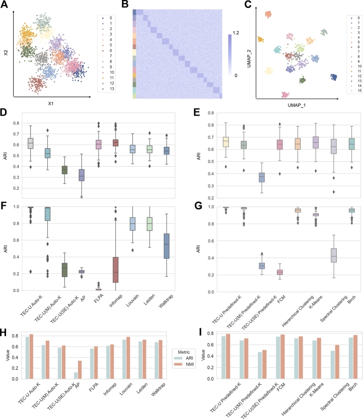 Figure 9
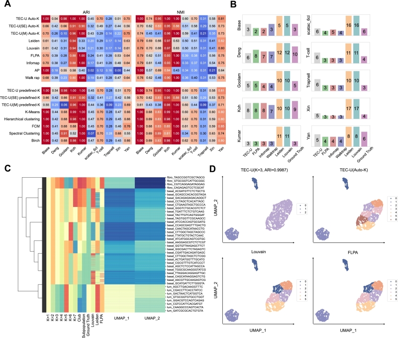 Figure 10
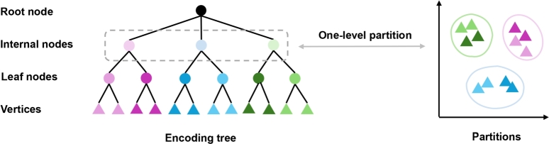 Figure 11
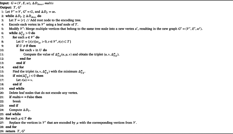 Figure 12
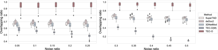 Figure 13
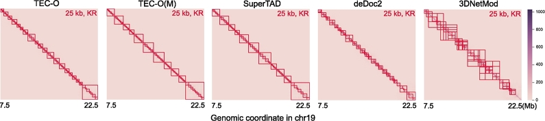 Figure 14
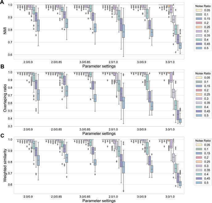 Figure 15
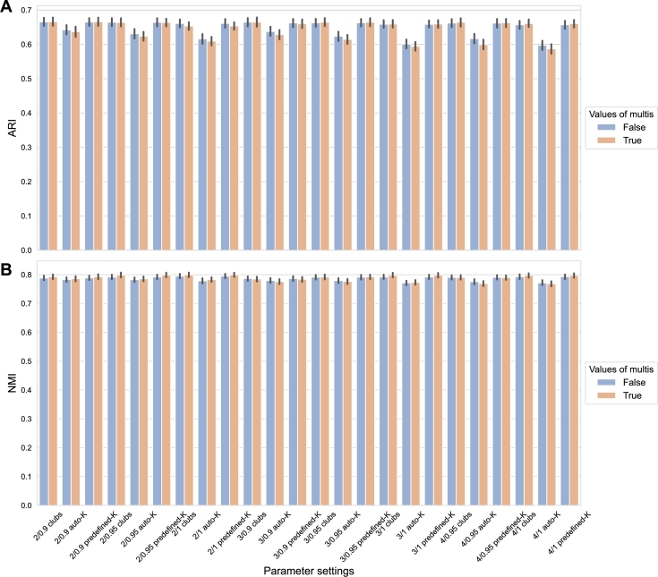 Figure 16
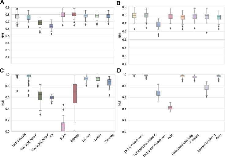 Figure 17
Peer Reviews
No public reviews on file for this paper yet. If you reviewed it on a platform where reviews are public (OpenReview, ICLR, NeurIPS, ICML), you can paste yours below so the community can read it here.
Videos
No videos yet. Explain this paper in a talk, walkthrough, or lecture? Add one.
Taxonomy
TopicsSingle-cell and spatial transcriptomics · Gene expression and cancer classification · Genomics and Chromatin Dynamics
Introduction
1
Entropy serves as a fundamental measure for quantifying the limits of information compression and provides a theoretical basis for exploring complex structures in large-scale graphs, applicable to both ordered and unordered graphs. An ordered graph is a symmetric graph where vertices are arranged in a specific linear order. The partitions of an ordered graph consist of consecutive vertices defined by this vertex ordering. In contrast, an unordered graph represents a more general structure that allows for arbitrary arrangements of vertices.
High-throughput Chromosome Conformation Capture (Hi-C) contact maps naturally form a genome-wide ordered graph of genomic regions. This characteristic enables the application of graph partitioning methods to identify topologically associated domains (TADs) from Hi-C contact matrices. The Hi-C technique [1] captures the ligated fragments and identifies the chromatin interactions. The pipeline presented in [2] transforms raw sequencing reads into a Hi-C contact map graph. As the fundamental units of the genome, TADs consist of continuous bins that interact more closely with each other than with bins from different TADs [3]. TADs are closely related to epigenetic and transcriptional activities [4], and variations in TAD boundaries can result in cancers and developmental disorders [5]. Therefore, accurate identification of TADs in Hi-C matrices warrants thorough exploration.
Recent advances have explored entropy-based graph partitioning strategies for TAD identification. Li et al. [6] developed a structural entropy-based method to identify structures with minimal perturbations caused by random variations and noise. They subsequently derived a greedy algorithm to identify TADs with minimal structural entropy through iterative merging and combining [7]. Norton et al. [8] applied a Louvain-like, locally greedy approach to TAD identification by optimizing network modularity using a single resolution parameter. Considering the order of bins, the Hi-C contact map can be represented as an ordered graph, allowing the use of dynamic programming (DP) method can be used to achieve the global optimal solution. Zhang et al. [9] designed a DP method to search for the encoding tree of the contact map graph with minimal structural entropy. Li et al. [10] developed deDoc2 to seek genome partitions with globally minimal structural entropy for both whole and local contact matrices. The success of structural entropy and DP in TAD identification motivates our exploration of new entropy metrics.
The functional diversity of cells results from genetic variation, biological evolution, and the differentiation of cellular structure and function. Constructing a cell hierarchy can help decipher the functional diversity. For instance, infiltrated lymphocytes in the tumor microenvironment are classified into T cells and B cells, with T cells further divided into cytotoxic T cells and helper T cells [11]. Recent advancements in single-cell sequencing technologies have provided opportunities for large-scale analyses in transcriptomics [12], genomics [13], and epigenomics [14]. These technologies have led to revolutionary insights into cellular heterogeneity and complexity, enabling the grouping of cells with similar molecular traits into the same category [15]. By performing clustering at the single-cell level, we can identify not only distinct cell subpopulations that provide broad categories, such as T cells and B cells, but also more specific groupings within these subpopulations, such as cytotoxic T cells and helper T cells.
Various methods have been employed for single-cell clustering, including Louvain [16], Leiden [17], Infomap [18], K-Means [19], Hierarchical Clustering [20], and Spectral Clustering [21]. Louvain and Leiden optimize modularity to identify clusters, while Infomap is an entropy-based method grounded in the map equation. Infomap can be sensitive to noise within the graph, potentially leading to incorrect community assignments in noisy graphs [22]. K-Means is a centroid-based partitioning algorithm that iteratively assigns data points to clusters by minimizing the within-cluster sum of squared distances. Hierarchical clustering constructs a tree-like dendrogram to represent nested clusters, while spectral clustering transforms data into a similarity graph, applying eigenvalue decomposition on the graph Laplacian for partitioning. These methods have been utilized in various studies [23], [24], [25], [26], [27]. Despite their widespread application, research on entropy-based methods for single-cell clustering remains insufficient. The aforementioned approaches either require a predefined number of clusters K or can determine the value of K only after computation, highlighting the need for a method that can simultaneously provide both functionalities.
In this study, we propose a novel metric named topology entropy to quantify the complexity of graphs, based on the concept of mutual information. We construct a topology entropy encoding tree to facilitate graph partitioning and develop Topology Entropy-based Clustering (TEC) methods for both ordered and unordered biological graphs. For ordered graphs, we present an optimal algorithm, TEC-O, which utilizes DP and operates in polynomial time. In contrast, for unordered graphs, we propose a heuristic algorithm, TEC-U, that constructs a topology entropy encoding tree in an agglomerative manner and employs DP to contract the hierarchical tree, yielding the corresponding partitioning results. Furthermore, we offer two modes for TEC-U: predefined-K and auto-K, depending on whether the value of K is predetermined. We validate our approaches utilizing both simulated and real datasets, including various resolution Hi-C contact matrices for GM12878, IMR90, K562, NHEK, and HMEC cell lines, high-resolution Micro-C interaction data, eight single-cell RNA sequencing (scRNA-seq) datasets, and two single-cell assay for transposase-accessible chromatin (scATAC) datasets incorporating gold standard cell type labels. Experiments demonstrate that topology entropy effectively encodes structural information, and our methods consistently outperform other approaches. Our source code is available at https://github.com/keyqing5/TEC.
Methods
2
In this section, we first introduce the theoretical foundation of our graph partitioning algorithms, including the construction of an encoding tree and the computation of the tree nodes within the encoding tree. We then define the notion of topology entropy and identify the optimal topology entropy encoding tree. For ordered graphs, we present TEC-O, a DP approach to find the optimal topology entropy encoding tree. In contrast, for more general unordered graphs, we propose a heuristic method, TEC-U, which constructs the topology entropy encoding tree in an agglomerative manner and employs DP to contract the hierarchical tree, yielding the corresponding partitioning results. Additionally, depending on whether the value of K needs to be predefined, we offer two modes: predefined-K and auto-K. Through TEC-O and TEC-U, we introduce a new metric to measure the dynamics and randomness of graphs, facilitating a comprehensive exploration of graph partitioning techniques. The overall workflow of our study is depicted in Fig. 1.Fig. 1. Workflow of clustering algorithms for ordered and unordered graphs. We developed distinct algorithms tailored for both ordered and unordered graphs. For ordered graph partitioning, the input is the adjacency matrix of the graph. Our TEC-O algorithm employs DP to construct a topology entropy encoding tree, which facilitates the identification of the optimal value of K. Conversely, for unordered graphs, the input is the sample-feature profile. Our TEC-U algorithm heuristically constructs a hierarchical encoding tree, followed by a contraction step for pruning. The predefined-K mode yields results based on a specified K, while the auto-K mode determines the optimal K and corresponding partitions automatically.Fig. 1
Definitions
2.1
Encoding tree
2.1.1
Let be a non-negative weighted graph, where V and E are the set of vertices and edges, respectively, , and . In this work, we assume the graphs are undirected. Let represent the weight of the edge connecting vertices u and v in G.
An encoding tree T of G indicates the hierarchical partitioning of the vertex set V. The root r of T represents, or encodes, the entire vertex set V. For notation simplicity, we denote graph vertices by u and v, and tree nodes by μ and ν. Each tree node μ encodes a vertex subset , . The children of each tree node partitions the vertices encoded by their parent node. For each vertex u, there exists a unique leaf node such that . Each leaf node encodes one or more vertices. An ideal encoding tree is hierarchical, where each tree node represents a partition with a finer resolution than that of its parent node. The vertices encoded by each tree node should exhibit a high degree of similarity.
Denote the volume of μ as the sum of weights of all vertices in , . For the volume of root r, we have . This indicates that the volume of r is equivalent to the volume of the entire graph G, which is defined as the sum of the weights of all edges in the edge set E. Define as the total weights of edges from vertices in to , . Suppose is the total weights of edges between vertices in , . We have . Clearly, if a tree node μ encodes one vertex, .
Topology entropy
2.1.2
Prior to defining our notion, it is worth recalling the modularity score [28] for a graph. Based on the formulation of the encoding tree, the definition of modularity can be rewritten as
where γ is a resolution parameter, finer resolution leads to more partitions, while coarser resolution leads to fewer partitions (the specific rewriting process is detailed in Appendix A).
Clearly, the first term in Eq. (1) can be interpreted as a joint distribution while the second term represents the marginal distribution , that is,
In this work, we define topology entropy or topology divergence, which utilize Kullback-Leibler (KL) divergence to measure the difference between joint distribution P and marginal distribution Q. The KL divergence is formulated as
We substitute and from Eq. (2) into Eq. (3) and take the negative of the entire equation. To address the issue of the limited scale of communities, we introduce parameters and into the definition, similar to γ in Eq. (1), resulting in the following formulation:
where and are resolution parameters that enable us to alter the relative weight given to the observed and randomized edge terms (the specific deviation process of Eq. (4) is detailed in Appendix B). The topology entropy of the root node r is 0, i.e., . With larger and , the method tends to identify larger communities. With smaller and , the method tends to identify smaller communities.
Let denote the topology entropy of the entire encoding tree. The value of is calculated as the sum of the topology entropy of all nodes in T, i.e., . The definition of topology entropy can be interpreted as the negative value of the KL divergence between P and Q. In Eq. (3), we need to maximize to obtain the optimal result. Therefore, our objective is to minimize the value of topology entropy, thereby reducing the global variance of the random walk on G. Finding the optimal topology entropy encoding tree can be further reformulated as finding a tree with the minimum topology entropy for graph G, that is
Based on the above, we transform the graph partitioning problem into the task of finding the optimal encoding tree with respect to topological entropy.
Finding the optimal solution on ordered graph
2.2
For ordered graph G, we can obtain the optimal solution using DP. Let represent the topology entropy of the optimal encoding tree that partitions vertices with k disjoint parts. Additionally, let denote the topology entropy of the tree node encoding vertices , . We define the recursive function to determine the optimal encoding tree for vertices with k leaves as
where
and
When calculating each value in D, the corresponding value of i is stored. During the backtracing process, we start from and retrieve the optimal value of i for partitioning the vertices. The backtrace continues until , at which node further partitioning of the vertices is no longer possible. If there is a need to limit the maximum number of partitions to K, the backtracing process can start from . In the final partition results, cases where or imply that no partitioning has occurred. Therefore, we exclude these cases when evaluating the optimal partition results.
There are possible values for , each of which can be computed in time. Therefore, calculation of H takes time . The size of the table storing is . Computing each value of needs time. Consequently, the time complexity of TEC-O of k leaves is .
The above discussion addresses a single layer of partitioning. To establish a hierarchical structure, we iteratively compute optimal partitions layer by layer using Eq. (6). Specifically, after obtaining the partitioning at a higher level, the current adjacency matrix is divided into multiple sub-matrices based on the identified boundaries. We then apply the same partitioning procedure to each sub-matrix to uncover the sub-partitioning structure. Importantly, when a TAD consists of only a few bins, we refrain from performing any further partitioning.
Finding the hierarchical solution on unordered graph
2.3
In this section, we consider extending our graph partitioning method from ordered graphs to unordered graphs. The input is converted into a more general sample-feature matrix. We aim to develop a graph partitioning (or clustering) algorithm that takes the sample-feature matrix as input and identifies the optimal topology entropy encoding tree. The algorithm could have significant applications in various problems, including constructing cell hierarchies. While clustering algorithms such as K-means [19] and Hierarchical Clustering [20] demand the exact value of K to be predefined before computation, algorithms such as Louvain [16] and Leiden [17] do not require K to be specified in advance; instead they reveal K value only after the clustering results are finalized. To address this limitation, TEC-U offers two optional modes: it can perform clustering with a predefined K or heuristically search for the optimal K. For convenience, we refer to these two modes as predefined-K mode and auto-K mode, respectively.
The input sample-feature profile is reduced dimensionality to form a matrix X, followed by the construction of a corresponding dense sample-sample similarity graph . The dense graph is constructed using a Gaussian kernel , where σ represents the standard deviation of X and quantifies the similarity between two samples. If the input is a low-dimensional matrix, further reduction is unnecessary, and we can move directly to the next step of processing. From the dense graph, a sparse graph is created using the k-nearest neighbors (kNNs) method, assigning binary edge weight. For nodes u and v, if either node is among the top k nearest neighbors of the other in the dense graph, the weight of the edge connecting them in the sparse graph is set to 1; otherwise, the weight is set to 0. Our clustering algorithm leverages both the sparse and dense graphs to perform calculations, ultimately identifying the optimal encoding tree with minimal total topology entropy. There are two primary approaches for tree construction: top-down and bottom-up. In the design of TEC-U, we chose an agglomerative approach due to its potential for improved local merges, which helps to avoid premature erroneous decisions.
Our clustering algorithm consists of four steps: initialization, merging phase, combination phase, and finding the optimal K for the hierarchical topology entropy encoding tree. In the initialization step, we add a root node r to the tree T, which has direct leaf nodes. Each leaf node t encodes a distinct vertex u from the graph , such that . The processing of the input and the details of each step are depicted in Fig. 2. Subsequently, we will describe each step thoroughly in the order presented.Fig. 2. Workflow of TEC-U clustering algorithm on unordered graph.Fig. 2
The merging phase consists of two nested iteration processes. Before detailing the iteration process, we need to explain the operation and properties of the tree nodes involved. We define two tree nodes, μ and ν, as connected when there exists at least one connecting edge between the vertices and in the encoded graph . For a vertex , we remove it from its current leaf node and instead assign it to a different leaf node , which is connected to μ. This results in new leaf nodes and , where and . We refer to this transformation as a merging operation. The change in the topology entropy value of the tree T before and after the merging can be computed as
If μ only encodes vertex u, then .
To facilitate discussion, we describe the two iterative processes as outer iteration and inner iteration. The inner iteration is used to perform merging at a more fine-grained resolution. In the inner iteration, for each vertex u in graph G, we compute the values for all possible candidates ν for merging resulting in a set of triples . We identify from the set of all triples, which indicates the vertex u and candidate ν. If , we proceed with the corresponding merging and continue iterating; if , we stop the iteration. Thus, in each iteration, a leaf node can exist in one of two states: remaining unchanged or undergoing merging. When the inner iteration ends, we remove all leaf nodes that do not encode any vertices.
The outer iteration then recalculates the difference in topology entropy between the encoding tree after one round of inner iteration and the encoding tree T before the iteration, denoted as . If , we merge all vertices associated with the same leaf node in into a single vertex, resulting in a new graph , and then start a new round of inner iteration. Otherwise, the iteration stops, and the process moves on to the combination phase.
Additionally, we have set a bool parameter called multis, which indicates whether to perform the outer iteration. When the parameter multis is set to False, it allows the algorithm to run only the inner iteration, thereby completing the basic fine-grained vertex merging operations. The selection of multis does not require manual setting. Our algorithm can operate with both possible values, running once for each, and subsequently select the appropriate partitioning outcome based on the topology entropy value of the encoding trees. More details on the merging phase are mentioned in Appendix D.
Through the merging phase, we obtain an encoding tree T with l leaf nodes and one root node r. In the combination phase, we further aggregate the leaf nodes to achieve a coarser partitioning result, facilitating the subsequent selection of K. Here, we define the combination operation: for tree nodes μ and ν, we construct their parent node ω, which is a child node of the root r. The change in the encoding tree topology entropy before and after a combination can be computed as
In the combination phase, we first iteratively combine the connected tree nodes μ and ν that yield the smallest value. Then, we relax the constraints on connectivity and select the tree node pair that produces the smallest for combination. The combination iterates until the upper hierarchy forms a complete binary encoding tree.
After the combination phase, we obtain a hierarchical encoding tree with tree nodes. Next, we perform a pruning-like operation on tree T to automatically select the optimal K value that minimizes the topology entropy value for dense graph G. We equate the task of finding the optimal encoding tree to that of identifying an aggregation of optimal subtrees. Consequently, the optimal partitioning of the entire graph is decomposed into multiple subproblems. Specifically, when looking for K partitions of G, it can be formulated as finding two subtrees encoding and partitions, where . Each tree node ω is treated as the root of a subtree . We identify the subtree with the minimum topology entropy for using DP, where is the maximum K value. For the subtree , assuming ω has two children, μ and ν, we have
where denotes the topology entropy of the subtree which effectively encodes a partition for vertices , and denotes the minimum topology entropy of the subtree with K children. Through the computation in Eq. (11), we generate a table that stores the values of . Additionally, we create a table storing the corresponding μ and ν, along with a cut-off table recording the corresponding for each minimum value obtained, i.e.,
During the backtrace process, we determine the optimal value of K as by
We then identify the children nodes μ and ν of the root based on table and , continue to determine the children nodes of μ and ν until the corresponding value in equals 1. Through this backtrace, we derive the optimal topology entropy encoding tree , which corresponds to the minimum topology entropy value for partitions. We then map the hierarchical structure of to the partitioning results of the graph G. It is worth mentioning that in the encoding tree generated by TEC-U, the tree nodes representing the K clusters do not necessarily reside at the same layer; however, the vertices they encode do not overlap.
In practical applications, for larger input data, it is possible to appropriately reduce the setting of values to decrease the running time of computation.
For a sparse graph with n vertices, initialization requires time. The time complexity of the merging phase is . In the combination phase, we use a heap to store the values of , resulting in a time complexity of , where . The process of selecting the optimal K using the DP tables has a time complexity of , where . Therefore, the overall time complexity of the TEC-U algorithm is .
Applying graph partitioning to TAD identification and single-cell clustering
2.4
A Hi-C contact map is equivalent to an ordered graph with its vertices arranged in a linear order. Each vertex in the graph indicates a bin (genomic region) in the contact map, and the edges represent the interaction frequencies between pairs of genomic bins. The linear order property allows us to employ efficient algorithms for further partitioning. Therefore, we apply the TEC-O algorithm described in Section 2.2 to the Hi-C contact matrix to identify the TADs.
Clustering analysis is routinely performed on single-cell sequencing data to explore and identify underlying cell identities. Constructing a cell hierarchy through cell clustering can help decipher the functional diversity of cells, which arises from genetic variation, biological evolution, and the differentiation of cellular structures and functions. Single-cell molecular data can be represented as a matrix, where the rows correspond to molecular features, such as genes or genomic regions, and the columns correspond to cells. Each matrix entry quantifies the value for a specific cell-feature pair, including measurements such as gene expression or copy number variation. Therefore, we input the cell molecular profiles and utilize the data processing procedure outlined in Section 2.3 to construct a cell-cell graph that captures the similarities between cells. This cell-cell graph is then applied to our algorithm, TEC-U, which facilitates cell clustering and represents the hierarchical relationships among the cells.
Results
3
Experiments on simulated ordered graph
3.1
Before conducting experiments with real data, we first validated the accuracy and robustness of TEC-O, using simulated ordered graph data. This allows us to assess the impact of different graph configurations on the results and compare TEC-O with other approaches.
We generated simulated Hi-C contact data incorporating different proportions of noise and TAD sizes. Specifically, the input is an adjacency matrix representing a graph with non-overlapping clusters, where . If edge , then ; otherwise, . The size (or length) of each TAD is indicated by the number of vertices contained within each cluster in the graph. We configured the vertices within each cluster to have a continuous adjacency relationship, ensuring a high probability of intra-interaction among the vertices to simulate the TADs observed in Hi-C contact data. Additionally, we established the presence of inter-interactions between different clusters to represent the noise in Hi-C contact data. The noise ratio is defined as the probability of inter-interaction relative to the probability of intra-interaction. A higher noise ratio indicates more edges between clusters, corresponding to increased noise. The number of TADs varies randomly between 8 and 10. We assigned a probability of 0.7 to the intra-connections within each cluster. Ground truth structures are obtained during generation. The simulation data are generated independently 100 times for each setting and input to all methods.
We compared the encoding trees corresponding to the inferred and ground truth TADs by calculating the values of weighted similarity [7] and overlapping ratio [9] (details in Appendix E). Both metrics evaluate the similarity between two encoding trees, with values ranging from 0 to 1. A value of 0 indicates no overlap between the two encoding trees, while a value of 1 indicates they are identical.
Before formally comparing with other baseline methods, we tested the impact of different values for parameters and in Eq. (4) on the experimental results. We set the deviation of TAD sizes to 3 and varied the noise ratio from 0.05 to 0.5. The combinations of and were set to (2.0, 0.9), (2.0, 0.85), (3.0, 0.85), (2.0, 1.0), (3.0, 0.9), and (3.0, 1.0). As shown in Fig. 3, the combination of and demonstrated the least sensitivity to noise in the data, leading to the best overall performance in terms of accuracy (more details in Fig. J.13). Therefore, we applied this parameter set in the subsequent experiments.Fig. 3. Comparison between different parameter settings (α1/α2) of topology entropy under various noise ratio. In the boxplot, the center line indicates the median of the metric, while the upper and lower boundaries of the box represent the third (Q3) and first (Q1) quartiles, respectively. The whiskers extend to 1.5 times the interquartile range (IQR, i.e., Q3 - Q1), and the points outside the whiskers represent outliers.Fig. 3
We compared results from SuperTAD [9], deDoc2 [10], and 3DNetMod [8]. These methods utilized structural entropy or modularity as their objective functions. Considering the performance of 3DNetMod in [9], we optimized it using DP to facilitate the comparison of different definitions of entropy. To validate the performance of our proposed topology entropy, we also replaced the topology entropy in TEC-O with modularity, denoted as TEC-O(M). All baseline methods were configured according to recommended or default parameters.
We evaluated the identification results of input matrices with varying noise ratios. The noise ratio was increased from 5% to 50% in increments of 5%, with the TAD size fixed at 10. As shown in Fig. 4A-B, when the noise ratio is less than or equal to 0.2, all methods achieve stable results with relatively high accuracy. However, as the noise increases, the accuracy significantly decreases, with notable changes in metrics at noise ratios of 0.25 and 0.3. When the noise ratio reaches 0.45 or higher, the performance of TEC-O(M) deteriorates significantly, with metric values approaching 0. At noise ratios of 0.4 and above, the results of deDoc2 and SuperTAD are similar, which we hypothesize is due to the inherent definition of entropy having a greater impact than differences in algorithm design. TEC-O, while showing a decrease in accuracy with increasing noise, maintains the highest average accuracy at a noise ratio of 0.5, with overlapping ratio and weighted similarity exceeding 0.7 and 0.8, respectively, outperforming other methods. Moreover, the accuracy of TEC-O is less affected by noise, demonstrating strong noise tolerance. The differences in metrics among the DP-based methods indicate that topology entropy can better assist in finding partitions close to the ground truth.Fig. 4. Robustness comparison under various noise ratios and deviations in TAD sizes. A-B. The x-axis denotes the noise ratio, increasing in 5% increments from 5% to 50%. C-D. The x-axis represents the deviation in TAD sizes, ranging from 1 to 5. The plots illustrate the distribution of specific metrics from 100 experiments under consistent parameter settings for input matrices. The box for TEC-O is colored dark red.Fig. 4
We also tested the effect of TAD size deviation on the performance of methods. With the noise ratio fixed at 0.3, we evaluated accuracy changes with TAD size deviations of . As shown in Fig. 4C-D, larger deviations in TAD size lead to a decrease in accuracy, particularly noticeable between 1 and 2. The overlapping ratio and weighted similarity of TEC-O remain very close to 1, with only a slight decrease in accuracy, outperforming the other methods.
Overall, the results for overlapping ratio and weighted similarity indicate that variations in noise ratio and TAD size deviation significantly impact the accuracy of identification. TEC-O demonstrates higher accuracy and better robustness compared to other approaches.
Furthermore, we explored the sub-TAD structures and compared the performance. To facilitate direct comparisons, we have retained the names of the methods introduced previously without modification.
For generating simulated data with two-level structures, we constructed TAD structures layer by layer and combined matrices from each layer. To facilitate comparison, we utilized the two-level results from baseline methods. We evaluated the identification results of the input matrices with varying noise ratios, increased from 5% to 50% in increments of 5%, while keeping the TAD size fixed at 10. As illustrated in Fig. F.11, TEC-O effectively partitioned the two-layer structures and demonstrated robustness against noise. In contrast, the TEC-O(M) method exhibited poor adaptability to the two-layer data and lacked robustness against noise. Notably, SuperTAD, deDoc2, and 3DNetMod showed comparable accuracy, with deDoc2 performing slightly better than the other two methods.
Real Hi-C contact data
3.2
We downloaded the processed real Hi-C contact dataset for chromosome 19 from the GM12878 and IMR90 cell lines at resolutions of 25 kb, 50 kb, and 100 kb, respectively [29]. The Hi-C contact matrices were derived from the normalized raw matrices using the Knight-Ruiz normalization method implemented in Juicer [2]. The start and end positions for the analysis were set at 7500000 bp and 22500000 bp, respectively. Additionally, we included datasets from K562, NHEK, and HMEC cell lines at a resolution of 25 kb, and conducted experiments with Micro-C data on human embryonic stem cells at resolutions of 5 kb and 10 kb. We aimed to evaluate the performance of methods across datasets with varying sequencing depths. Micro-C, as a high-resolution variant of Hi-C, enables a more detailed analysis of TADs. The Hi-C contact data for the cell lines were obtained from [29], while the Micro-C dataset was retrieved from [30] with accession number 4DNES21D8SP8, analyzed from positions 7500000 bp to 9300000 bp.
Furthermore, we generated subsamples of the contact data from the K562 cell line at different ratios (30%, 50%, and 70%) by randomly downsampling the pooled sample to further assess the robustness of methods. Specifically, downsampling was performed using FAN-C [31], resulting in normalized interaction matrices at a resolution of 25 kb.
Comparison of length and contact density of identified TADs
3.3
For the TADs identified in the real Hi-C contact matrices, we first calculated the TAD length (size) and contact density [7] distribution for each cell line using different methods. If the length of a TAD is too small, it may be filtered out in subsequent biological analyses. The contact density is calculated by dividing the sum of contacts within a TAD by the length of that TAD [7]. A high contact density of the identified TADs indicates that the quality of the TADs detected is high.
As illustrated in Fig. 5A, TEC-O detects TADs with longer lengths for the GM12878 cell line. The results obtained from TEC-O demonstrate that our entropy definition effectively prevents TADs from being excessively small, ensuring they are retained for analysis. For the GM12878 cell line, the lengths of TADs identified by 3DNetMod exhibit the smallest median value among all methods. Despite a wide range of lengths observed in 3DNetMod, with the largest TAD length for the IMR90 cell line, the contact density of the TADs identified by 3DNetMod, both in terms of maximum and median values, is lower than the corresponding values obtained using TEC-O. This observation suggests a potential instability in 3DNetMod. As shown in Fig. 5B, the median value of contact density of the TADs identified by TEC-O is the highest among all methods.Fig. 5. The TAD attribute statistics for all methods using a 25 kb resolution real Hi-C contact matrix on chromosome 19 for GM12878 and IMR90 cell lines. Box plots illustrate the inferred TADs regarding A. TAD length and B. contact density. Each boxplot illustrates the distribution of values for methods associated with a specific cell line. C and E. The fold change values of peak numbers of structural proteins (CTCF, RAD21, and SMC3) in peak regions compared to background regions. D and F. Cumulative bar charts displaying the proportions of TADs enriched for H3K27me3 or H3K36me3 (FDR corrected p-value ≤0.1), and those with no significant enrichment (i.e., FDR >0.1).Fig. 5
Enrichment of epigenetic characteristics at TAD boundaries or in TADs
3.4
The chromatin insulator protein CTCF and the cohesin complex, SMC3 and RAD21, are known to be enriched at TAD boundaries [29]. To assess this enrichment, we analyzed the binding of CTCF, SMC3, and RAD21 using ChIP-seq data. We quantified the enrichment by calculating the average fold change of peak enrichment between TAD boundaries and their flanking regions. The fold change was determined as the ratio of the number of peaks at TAD boundaries to those in the flanking regions, minus 1. Specifically, we calculated the number of peaks around TAD boundaries (±1 bin) and defined the flanking regions as 100 kb segments located 400 kb away from the boundaries. A high average fold change indicates significant protein enrichment at the boundaries, while a value of zero suggests no enrichment. We retrieved peak data for cells from the ENCODE (http://www.encodeproject.org).
As shown in Fig. 5C and E, boundaries identified by TEC-O exhibited higher fold changes for all structural proteins across both cell lines compared to other methods.
For GM12878 and IMR90 cell lines, we further evaluated the enrichment of histone modifications H3K27me3 and H3K36me3, following the analysis from [9], [32]. We computed the ratio of enrichment for either histone mark within each TAD by grouping ChIP-seq signals into intervals corresponding to 10% of the average TAD size. For each interval, we calculated the log10-ratio (LR) between H3K27me3 and H3K36me3. The average LR values were derived as the observed LR values, and the intervals were shuffled 1000 times to establish the distribution of LR values. We then calculated empirical p-values for TADs and adjusted the p-values for the false discovery rate (FDR) using the Benjamini-Hochberg procedure. We reported the ratio of enrichment with FDR-corrected p-values ≤0.1. A TAD was considered to show no enrichment for either histone mark if the FDR-corrected p-value exceeded 0.1. As illustrated in Fig. 5D and F, TEC-O identified a greater proportion of TADs with enriched histone modifications compared to other methods. Moreover, the proportion of TADs identified by TEC-O that were not enriched for either histone mark was the smallest among all methods. For more details, please refer to Table H.5, Table H.6, Table H.7, Table H.8.
For the K562, NHEK, and HMEC cell lines, as well as Micro-C contact data, we assessed the enrichment of regulatory elements, including CTCF, H3K27ac, H3K4me3, and H3K9me3. We found that CTCF, H3K4me3, and H3K27ac were enriched at TAD boundaries, while H3K9me3 was depleted. We evaluated the accuracy of the methods by calculating the fold change of these regulatory elements. The accession numbers are summarized in Table G.3, Table G.4.
As presented in Table I.9, Table I.10, TAD boundaries identified by TEC-O displayed enrichment across most regulatory elements, demonstrating the effectiveness of our algorithm and the utility of topology entropy in TAD identification.
As shown in Table I.11, the boundaries of TADs inferred from 100% of the total reads and those inferred from various ratios of downsampled reads became increasingly similar as sequencing depth increased for most callers. We quantified the similarity between TADs inferred from 100% of the reads and those from downsampled ratios using the overlapping ratio and weighted similarity metrics. The results from TEC-O demonstrate its robustness in TAD identification.
For TAD structures with two levels, we tested the methods on the Hi-C contact matrix for the K562 cell line. As shown in Table F.2 and Fig. F.12, TADs identified by TEC-O exhibited high enrichment for CTCF, SMC3, and H3K4me3. Notably, during the two-layer analysis, the results from 3DNetMod were comparable to those from SuperTAD and deDoc2.
For Micro-C contact matrices, as illustrated in Fig. 6, TEC-O identified TADs with greater average contact density. The results from deDoc2 and SuperTAD, both of which are based on structural entropy, were similar. After filtering, TADs identified by 3DNetMod were reduced to only 3 and 7 for the two resolutions. Regarding consistency across different resolutions, both TEC-O and SuperTAD produced robust results. Additionally, in Table I.12, TEC-O achieved higher fold change values for regulatory elements, including CTCF, H3K4me4, and RAD21, at both 5 kb and 10 kb resolutions.Fig. 6TAD identification on Micro-C data. A. Heatmaps of Micro-C contact data (chr19:7500000-9300000bp). Inferred TAD boundaries are annotated with resolution-specific colors (5 kb in red, 10 kb in blue). B-D. Boxplots and bar plots illustrate the inferred TADs regarding B. TAD length, C. contact density, and D. number of TADs. E. Consistency evaluation between 5 kb and 10 kb resolutions using overlapping ratio and weighted similarity.Fig. 6
Consistency between TAD boundaries at different resolutions
3.5
We evaluated the robustness and consistency of methods by comparing the similarity of TAD boundaries at different resolutions for cell lines. Specifically, we input Hi-C matrices with identical starting and ending sites on chromosome 19 at different resolutions into TEC-O and compare the similarity of TAD boundaries both qualitatively and quantitatively.
The heatmaps of the input matrices for two cell lines, along with the identified TAD boundaries at 25 kb, 50 kb, and 100 kb resolutions, are depicted in Fig. 7. It is observable that when the input data resolution is finer, the methods tend to yield smaller domains. The differences among TEC-O, TEC-O(M), and SuperTAD in identifying TAD boundaries highlight the impact of the different definitions of entropy. 3DNetMod exhibits significant inconsistency in results across different resolutions due to excessive boundary duplications, leading to discontinuous filtered domains. In contrast, TEC-O demonstrates overall better consistency.Fig. 7. Consistency comparison for methods. We plotted the heatmap of the Hi-C contact matrix used as input and the inferred TAD boundaries for GM12878 (first two rows) and IMR90 (last two rows) cell lines. TAD boundaries are shown in the upper and lower triangles, with text within these triangles indicating the resolution and KR normalization of the corresponding input matrix. When comparing results across two resolutions, the domains calculated at a finer resolution are shown in red, while those at a coarser resolution are shown in blue. In each heatmap, the similarity between the boundaries reflects the consistency of the method across the matrices of these two resolutions.Fig. 7
To quantify the consistency, we calculated the weighted similarity, normalized mutual information (NMI), and overlapping ratio for the TAD boundaries at different resolutions. As shown in Table 1, all methods exhibit a relatively high consistency in the comparisons between 25 kb and 50 kb for GM12878, as well as between 50 kb and 100 kb for IMR90. Due to the duplications in boundaries and the filtering settings, 3DNetMod consequently shows vast disagreement between results. Among all results, TEC-O demonstrates higher consistency in outputs for both GM12878 and IMR90 cell lines across different resolutions. TEC-O demonstrates higher consistency compared to TEC-O(M), further validating the robustness of our topology entropy approach and its applicability in addressing TAD detection challenges.Table 1. Evaluation of similarity criteria between results at 25 kb, 50 kb, and 100 kb resolutions across all methods.Table 1. Cell LineMetricMethodTEC-OTEC-O(M)SuperTADdeDoc23DNetModGM1287825/50OR^**^0.96140.96710.95850.91310.9063WS0.97580.96930.97090.93850.9717NMI0.96750.96780.94790.94150.8923 GM1287850/100OR0.91740.81360.93280.86390.8546WS0.93740.88660.95450.90680.9574NMI0.93980.92480.93960.93430.8748 IMR9025/50OR0.90420.79900.91060.70040.8108WS0.93430.87840.94570.82260.8670NMI0.94120.92960.94070.90780.7598 IMR9050/100OR0.90690.89950.89900.91810.8861WS0.93200.93100.93770.93770.9556NMI0.94610.94100.91710.94100.9072 25/50: agreement of 25 kb v.s. 50 kb; 50/100: agreement of 50 kb v.s. 100 kb^**^ OR=overlapping ratio; WS=weighted similarity
Experiments on simulated unordered graph
3.6
We generated two types of input data: two-dimensional and higher-dimensional datasets, to evaluate the algorithmic framework of TEC-U and assess topology entropy as an objective measure. Specifically, the higher-dimensional dataset refers to high-dimensional matrices processed into cell-cell similarity graphs. Examples of these two types of input data are shown in Fig. 8A and B.Fig. 8. Performance comparison of methods on two types of simulated datasets. A. A two-dimensional input matrix. B. A higher-dimensional input matrix. C. UMAP dimensionality reduction of the matrix from B. The colors of the points in A and C, along with the colored bars on the left side of B, indicate the different clusters obtained by TEC-U. D-G. The ARI distributions of the methods under predefined-K and auto-K modes, respectively, after conducting 100 repeated experiments on the two-dimensional data in D-E and the higher-dimensional data in F-G. H-I. The averaged ARI and NMI values of the methods under auto-K and predefined-K modes, respectively, after 100 repeated experiments on the simulated single-cell data.Fig. 8
For the two-dimensional data, we generated isotropic Gaussian blobs for clustering. We fixed the number of clusters at 14, with each cluster containing 150 members and a standard deviation of 1.2. In contrast, the higher-dimensional data were simulated under different settings to mimic single-cell sequencing data. The simulated input matrix was initialized with randomly generated values ranging from 0 to 1. For each cell cluster, we designated approximately 20 marker genes (ranging from 8 to 32 across our experiments). Specifically, for cells in cluster C, certain genes exhibited expression values that were moderately higher than those of cells outside the cluster. Our goal was to compare methods that leverage features represented by these marker genes. To increase complexity, some expression values within the cluster were allowed to be lower than those outside, with the range set from 0.5 to 1.2. The higher-dimensional data comprised 16 clusters, each containing between 40 and 60 members (or cells). The simulation data were generated independently 100 times under each setting and subsequently input into all methods.
For comparison, we calculated the Adjusted Rand Index (ARI) [33] with respect to the ground truth to measure the concordance (details in Appendix E). ARI values range from -1 to 1, where an ideal clustering achieves an ARI value of 1, and a value close to 0 indicates random clustering. For details on parameter settings, please see Fig. J.14.
We compared the results from several clustering algorithms, including Louvain, Leiden, Walktrap [34], FLPA [35], Affinity Propagation (AP) [36], and Infomap for the auto-K mode; Fuzzy C-Means (FCM) [37], Hierarchical Clustering, K-Means, Spectral Clustering, and Birch [38] for the predefined-K mode. For predefined-K mode, K was provided with the ground truth value. To validate the effectiveness of our proposed topology entropy and the overall performance of our algorithmic framework, we substituted the topology entropy in TEC-U with modularity and structural entropy, resulting in TEC-U(M) and TEC-U(SE), respectively. All baseline methods utilized their recommended or default parameters, requiring input in the form of a kNN graph or other specified formats; thus, data were processed accordingly. The value of in the merging phase of TEC-U was set to 0.0000001.
As shown in Fig. 8, in auto-K mode, Louvain, Leiden, and TEC-U achieved higher average ARI scores on higher-dimensional data, while FLPA and Infomap demonstrated better performance on the two-dimensional data. In predefined-K mode, for two-dimensional data, the performance of all methods was relatively similar, with the exception of the one using structural entropy, with TEC-U performing slightly better than K-Means. For higher-dimensional data, FCM and Spectral Clustering showed a significant decline in performance, while Hierarchical Clustering, K-Means, Birch, and TEC-U demonstrated higher accuracy. For higher-dimensional data, the median ARI of TEC-U was higher than that of other methods in both auto-K and predefined-K modes. Even when using the same objective function, modularity, TEC-U(M) achieved a higher median ARI compared to Louvain and Leiden, validating the efficiency of TEC-U's design. Additionally, the comparison indicates that under the same algorithmic framework, the definition of topology entropy can better facilitate accurate clustering. Results of NMI scores are provided in Fig. K.15.
To further evaluate the performance on single-cell clustering, simulated single-cell data were generated using splatter [39], using the following parameters: three cell populations, nGenes , group.prob = c(0.4, 0.3,0.3), and path.from=c(0,0,1). The sizes of the datasets were 100, 300, 500, 1000, 2000, 5000, and 10,000, respectively. Simulated data of each size are generated randomly 100 times. The ground truth cell populations were obtained during generation. As shown in Fig. 8H and I, TEC-U achieved higher accuracy in both modes (further details in Table K.13, Table K.14). Additionally, the performance of TEC-U was compared with results obtained without utilizing sparse and dense graphs generated during the graph construction process. The results presented in Table K.15, Table K.16 demonstrate the effectiveness of graph construction in TEC-U.
Determining cell hierarchy on scRNA and scATAC data
3.7
For experiments, we collected eight scRNA-seq datasets and two scATAC-seq datasets. The scRNA-seq datasets include those from Yan [40], Deng [41], Biase [42], Goolam [43], Koh [44], Kumar [45], Trapnell [46], and Xin [47]. We downloaded the expression profiles and corresponding cell labels for the scRNA-seq data (accession codes are summarized in Appendix G), and performed dimensionality reduction using UMAP [48]. For the scATAC-seq datasets, namely scatac_6cl [49] and T-cell [50], we utilized processed accessibility profiles and cell labels from scOpen [51], which were also reduced in dimensionality using UMAP. Regarding the TEC-U algorithm, we recommend processing the raw data to obtain low-dimensional embeddings as input.
To evaluate the performance of the methods in cell subpopulation detection, we used ARI and NMI as metrics for clustering accuracy. Comparisons were conducted for both predefined-K and auto-K modes. As illustrated in Fig. 9A, TEC-U, utilizing topology entropy, outperforms or matches the accuracy of other methods across most datasets, except for Xin and Yan. Even in the auto-K mode, our algorithm framework, which employs modularity and structural entropy as the objective function, demonstrates high accuracy. Additionally, it is evident that TEC-U exhibits overall stability in accuracy, without the significant discrepancies between maximum and minimum accuracy observed in methods such as AP and Spectral Clustering. Louvain and Leiden show very similar performance across all datasets. In Fig. 9B, it is evident that across the ten datasets we used, Louvain and Leiden tend to produce far more clusters than the ground truth, resulting in lower clustering accuracy. In contrast, TEC-U yields K values in the auto-K mode that are closer to the ground truth.Fig. 9. Applying methods to scRNA and scATAC datasets. A. The ARI and NMI scores of the methods in auto-K and predefined-K modes for each dataset. Darker red indicates higher metric values, while darker blue indicates lower values. B. The number of subpopulations detected by the methods for each dataset in auto-K mode. C. The clustering results on the p3cl dataset of TEC-U corresponding to different predefined K values. UMAP dimensionality reduction was performed on the p3cl data. The term club refers to the result of only conducting the merging phase in TEC-U. For comparison, the ground truth and the clustering results of Louvain, Leiden, and FLPA are also included. D. UMAP plots of the p3cl dataset, with cells colored by clusters. The ARI score of TEC-U is 0.9987.Fig. 9
To further observe and compare the results of cell subpopulation detection, we applied methods to the p3cl dataset [52], which includes three cell lines: human dermal fibroblasts, the breast cancer luminal epithelial cell line MCF-7, and the breast cancer basal-like epithelial cell line MDA-MB-468, all obtained through 10x single-cell sequencing, comprising a total of 2,609 cells. As shown in Fig. 9C-D, the clustering result of TEC-U is closer to the ground truth and can simultaneously provide finer resolution cell clusters based on subpopulations, thereby constructing a cell hierarchy.
Conclusion
4
In this study, we introduce topology entropy, which quantifies the complexity of networks. To facilitate graph partitioning for both ordered and unordered biological graphs, we developed the encoding tree with minimal topology entropy. For ordered graphs, we present an optimal algorithm named TEC-O, which leverages DP and operates in polynomial time. For unordered graphs, we design a heuristic algorithm called TEC-U, which constructs the topology entropy encoding tree in an agglomerative manner and employs DP to contract the hierarchical tree, yielding the corresponding partitioning results. Additionally, TEC-U offers two operational modes, depending on whether the value of K is specified in advance. We validate our approaches using both simulated and real datasets. TEC-O and TEC-U are tested across various noise ratios and cluster sizes on simulated data. Performance comparisons demonstrate that our topology entropy metric effectively encodes structural information, providing a robust foundation for knowledge discovery from noisy data. Experiments on real Hi-C and single-cell sequencing data demonstrate that our methods outperform other baseline approaches and yield biologically meaningful results.
In future research, we aim to provide a more comprehensive theoretical analysis of the definition of topology entropy and investigate its accessibility and robustness as a metric. Furthermore, we plan to explore additional applications in biological problems to expand the utility of our proposed methods.
CRediT authorship contribution statement
Qiushi Liang: Writing – review & editing, Writing – original draft, Validation, Software, Methodology, Investigation, Formal analysis. Shengjie Zhao: Writing – review & editing, Project administration, Funding acquisition. Lingxi Chen: Writing – review & editing, Investigation. Shuai Cheng Li: Writing – review & editing, Project administration, Methodology, Conceptualization.
Declaration of Competing Interest
None.
The reference list from the paper itself. Each links out to its DOI / PubMed record.
- 1Lieberman-Aiden E.Van Berkum N.L.Williams L.Imakaev M.Ragoczy T.Telling A.Comprehensive mapping of long-range interactions reveals folding principles of the human genome Science 326595020092892931981577610.1126/science.1181369 PMC 2858594 · doi ↗ · pubmed ↗
- 2Durand N.C.Shamim M.S.Machol I.Rao S.Huntley M.H.Lander E.S.Juicer provides a one-click system for analyzing loop-resolution hi-c experiments Cell Syst 312016959810.1016/j.cels.2016.07.002https://www.sciencedirect.com/science/article/pii/S 240547121630219827467249 PMC 5846465 · doi ↗ · pubmed ↗
- 3Pope B.D.Ryba T.Dileep V.Yue F.Wu W.Denas O.Topologically associating domains are stable units of replication-timing regulation Nature 515752720144024052540983110.1038/nature 13986 PMC 4251741 · doi ↗ · pubmed ↗
- 4Ye Y.Gao L.Zhang S.Mstd: an efficient method for detecting multi-scale topological domains from symmetric and asymmetric 3d genomic maps Nucleic Acids Res 47112019 e 6510.1093/nar/gkz 201PMC 658233830941409 · doi ↗ · pubmed ↗
- 5Spielmann M.Lupiáñez D.G.Mundlos S.Structural variation in the 3d genome Nat Rev Genet 19720184534672969241310.1038/s 41576-018-0007-0 · doi ↗ · pubmed ↗
- 6Li A.Pan Y.Structural information and dynamical complexity of networks IEEE Trans Inf Theory 626201632903339
- 7Li A.Yin X.Xu B.Wang D.Han J.Wei Y.Decoding topologically associating domains with ultra-low resolution Hi-C data by graph structural entropy Nat Commun 91201832653011188310.1038/s 41467-018-05691-7PMC 6093941 · doi ↗ · pubmed ↗
- 8Norton H.K.Emerson D.J.Huang H.Kim J.Titus K.R.Gu S.Detecting hierarchical genome folding with network modularity Nat Methods 152201811912210.1038/nmeth.456029334377 PMC 6029251 · doi ↗ · pubmed ↗